Gravitational Waves from Spinning Compact Binaries

Abstract

Binary systems of rapidly spinning compact objects, such as black holes or neutron stars, are prime targets for gravitational wave astronomers. The dynamics of these systems can be very complicated due to spin-orbit and spin-spin couplings. Contradictory results have been presented as to the nature of the dynamics. Here we confirm that the dynamics - as described by the second post-Newtonian approximation to general relativity - is chaotic, despite claims to the contrary. When dissipation due to higher order radiation reaction terms are included, the chaos is dampened. However, the inspiral-to-plunge transition that occurs toward the end of the orbital evolution does retain an imprint of the chaotic behaviour.

Gravitational wave astronomy blurs the lines between theory and observation by requiring accurate source modeling to facilitate detection. While it is possible to detect gravitational waves without precise waveform templates, matched filtering against a template bank is the only way to extract detailed information about the sources. A template based, matched filtering approach to gravitational wave data analysis is impractical if the orbital dynamics is chaotic ms ; jj1 ; njc2 ; jj2 . Systems that exhibit sensitive dependence to initial conditions require template banks that are exponentially larger than those of non-chaotic systems.

Spinning compact binaries pose a challenge to template based detection and parameter extraction techniques. The waveforms depend on a large number of parameters, including the masses of the two bodies, their spins, and the relative alignment of the spin and orbital angular momentum - some 11 parameters in all. Even with a relatively coarse sampling of parameter space, the resulting template bank can be very large. The hope is that hierarchical schemes can be used that start with a coarse sampling and proceed by successive refinement. However, template based methods, hierarchical or otherwise, will not work if the underlying dynamics is chaotic. The sensitivity to initial conditions that characterizes chaotic systems ensures that waveforms that are initially nearby (as measured by their cross correlation over some time interval) will diverge exponentially with time njc2 .

A debate has arisen as to whether spinning compact binaries exhibit chaotic behaviour. The first indication of chaotic behaviour was found using a test particle approximation ms , but chaotic orbits were only found for unphysically large values of the particle’s spin. The problem was also approached using the post-Newtonian approximation to general relativity, and fractal methods were used to show that binaries with realistic spins exhibited chaotic behaviour jj1 . Commentaries were written emphasizing that radiation reaction would damp the chaos njc1 , and that the post-Newtonian approximation was being pushed beyond its domain of validity scott , although unavoidably since no better approximation is available. However, neither commentary disputed the central result of Refs. jj1 ; jj2 - that the second post-Newtonian (2PN) equations of motion admit chaotic behaviour. Then a paper was published “ruling out chaos in compact binary systems”ras . This study used the same 2PN equations of motion, but a different method for establishing chaos - Lyapunov exponents rather than fractals. The results reported in Refs.jj1 and ras sit in stark contrast. The trajectories that form the fractal basin boundaries found in jj1 belong to a set of unstable periodic orbits know as the strange repellor. These orbits must have positive Lyapunov exponents. Trajectories near the boundaries will also have positive Lyapunov exponents, as may orbits that lie far from the boundaries.

In what follows, we refute the claims made in Ref.ras by showing that the 2PN equations of motion do admit orbits with positive Lyapunov exponents. We then explore the significance of this result by comparing three key timescales in the problem - the average orbital period $T_{o}$, the Lyapunov time $T_{\lambda}$, and the decay time $T_{d}$. If $T_{\lambda}$ is short compared to $T_{d}$, the chaotic dynamics seen in the conservative 2PN dynamics will leave a strong imprint on the 2.5PN dissipative dynamics.

The post-Newtonian equations of motion are written as a series expansion in $v^{2}/c^{2}$, where $v$ is the relative velocity and $c$ is the speed of light:

$$\mu\ddot{\bf r} = {\bf F}_{N}^{(0)}+{\bf F}_{PN}^{(1)}+{\bf F}_{SO}^{(1.5)}+{\bf F}_{PN}^{(2)}+{\bf F}_{SS}^{(2)}+{\bf F}_{QM}^{(2)}$$ (1)

$$+{\bf F}_{RR}^{(2.5)}+{\bf F}_{SO}^{(2.5)}+{\bf F}_{PN}^{(3)}+{\bf F}_{SS}^{(3)}+\dots$$

Here $\mu=m_{1}m_{2}/M$ is the reduced mass, $M=m_{1}+m_{2}$ is the total mass, and $\ddot{\bf r}$ is the relative acceleration of the two bodies. The product $\mu\ddot{\bf r}$ is given in terms of a series of forces, starting with the usual Newtonian force ${\bf F}_{N}^{(0)}=m_{1}m_{2}{\bf r}/r^{3}$. The superscripts denote the order of the post-Newtonian expansion and the subscripts denote the type of force. The explicit form of the higher order terms can be found in Refs.kidder ; poisson ; too . Qualitatively, the 1PN force ${\bf F}_{PN}^{(1)}$ introduces perihelion precession. The 2PN force ${\bf F}_{PN}^{(2)}$ introduces isolated unstable orbits, along with an inner most stable circular orbit (ISCO), and the possibility of merger. The 1.5PN spin-orbit force ${\bf F}_{SO}^{(1.5)}$ leads to precession of the orbital plane, as do the 2PN spin-spin ${\bf F}_{SS}^{(2)}$ and spin-induced quadrupole-monopole ${\bf F}_{QM}^{(2)}$ forces. The spin-spin force is attractive for spins that are aligned and repulsive for spins that are anti-aligned. The 2.5PN order radiation reaction force, ${\bf F}_{RR}^{(2.5)}$, is the first non-conservative term, and it causes the orbital energy $E$ and angular momentum $\bf L$ to decay. Associated with the spin-orbit and spin-spin forces are torques that act on the spin of each body, causing the spins to precess - see Ref.kidder for details. While the expansion is known to 3PN order, we will only consider terms up to 2.5PN order to facilitate comparison with the results in Refs.jj1 ; ras . For the same reason, we also neglect the 2PN quadrupole-monopole and 2.5PN spin-orbit forces. In defense of these approximations, we point out that the terms that we keep capture the main qualitative features expected from full general relativity. If anything, the higher order non-dissipative terms are likely to increase the strength of the chaotic behaviour.

The dynamics takes place in a 12-dimensional phase space with coordinates $\vec{X}=({\bf x},{\bf p}_{x},{\bf S}_{1},{\bf S}_{2})$, where ${\bf p}_{x}$ is the momentum conjugate to ${\bf x}$, and ${\bf S}_{i}$ describes the spins of the two bodies. In the absence of radiation reaction there are 6 conserved quantities, the energy $E$, total angular momentum ${\bf J}={\bf L}+{\bf S}_{1}+{\bf S}_{2}$ and spin magnitudes $|{\bf S}_{i}|$. Linearizing the equations of motion about a reference trajectory $\vec{X}(t)$ gives the evolution of the difference ${\delta\vec{X}}(t)$

$$\delta\dot{X}_{i}(t)=\left.\frac{\partial\dot{X}_{i}}{\partial X_{j}}\right|_{\vec{Y}(t)}\!\delta X_{j}(t)\equiv K_{ij}(t)\delta X_{j}(t)\,.$$ (2)

The solution to this equation can be written:

$$\delta X_{i}(t)=L_{ij}(t)\delta X_{j}(0)\,.$$ (3)

The evolution matrix $L_{ij}(t)$ is given in terms of the linear stability matrix $K_{ij}$ by

$$\dot{L}_{ij}=K_{il}L_{lj}\,,$$ (4)

with $L_{ij}(0)=\delta_{ij}$ (repeated indices imply summation). The Lyapunov exponents are defined in terms of the eigenvalues $\Lambda_{i}(t)$ of the distortion matrix $\Lambda_{ij}=L_{il}L_{lj}$:

$$\lambda_{i}=\lim_{t\rightarrow\infty}\frac{1}{2t}\log\Lambda_{i}(t)\,.$$ (5)

The 2PN equations of motion are conservative and can be derived from a Hamiltonian. The expansion and vorticity of the flow vanishes for Hamiltonian systems (in canonical coordinates), so that ${\rm det}(\Lambda_{ij})=1$, $\Lambda_{ij}=\Lambda_{ji}$ and the Lyapunov exponents come in $+/-$ pairs that measure the exponential shearing of the flow. The principal Lyapunov exponent $\lambda_{p}={\rm max}(\lambda_{i})$ can be calculated without directly isolating the eigenvalues from

$$\lambda_{p}=\lim_{t\rightarrow\infty}\frac{1}{2t}\log\left(\frac{\Lambda_{jj}(t)}{\Lambda_{jj}(0)}\right)\,.$$ (6)

In the limit of very long times, the principal positive Lyapunov exponent will dominate the trace in eqn. 6.

By contrast, the quantity calculated in Ref.ras was

$$\lambda_{d}=\lim_{t\rightarrow\infty}\lim_{dX(0)\rightarrow 0}\frac{1}{t}\log\left(\frac{dX(t)}{dX(0)}\right)$$ (7)

with $dX=((X_{i}(t)-Y_{i}(t))(X_{i}(t)-Y_{i}(t)))^{1/2}$ the Cartesian distance between the 12-component vectors of a reference trajectory $\vec{X}(t)$ and a nearby shadow trajectory $\vec{Y}(t)$. It must be emphasized that this is not a Lyapunov exponent. Eqn. 7 will automatically yield zero when the limit $t\rightarrow\infty$ is taken. However, eqn. 7 can represent an approximation to the Lyapunov exponent if an additional rescaling of the shadow trajectories is incorporated. The rescaling is accomplished by determining when $dX(t_{r})>R\,dX(0)$ for some threshold $R$, then starting a new shadow trajectory $\vec{Y}^{\prime}(t)$ with initial conditions

$$\vec{Y}^{\prime}(t_{r})=\vec{X}(t_{r})+\left(\vec{Y}(t_{r})-\vec{X}(t_{r})\right)/R\,.$$ (8)

The rescaling is repeated throughout the evolution to ensure that one is accurately approximating the stability of the reference trajectory $X(t)$. The problem with this method is that the choice of threshold can significantly affect the value of $\lambda_{d}$. It is possible that the apparent absence of rescaling in Ref. ras is the source of our disagreement. A far more robust method is to evolve the perturbation $\delta\vec{X}(t)$ directly using eqn. 2. No rescaling is needed as eqn. 2 defines the dynamic stability without approximation.

A second more subtle point to make regarding eqn. 7 is that while $dX(t)$ is often referred to as the “distance between nearby trajectories in phase space”, this statement is misleading as phase space does not admit a metric structure. Even if rescaled properly so that $dX(t)\approx\delta X(t)$ from eqn. 2, the distance $dX(t)$ only measures the projection of the distortion matrix onto the initial displacement vector:

$$d^{2}X(t)\approx d^{2}(t)=dX_{i}(0)\Lambda_{ij}(t)dX_{j}(0).$$ (9)

As a consequence of this additional approximation, $\lambda_{d}$ provides only a lower bound for $\lambda_{p}$.

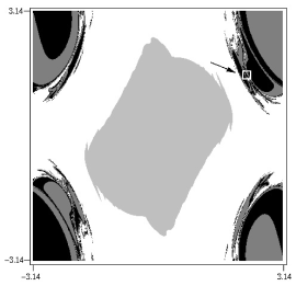
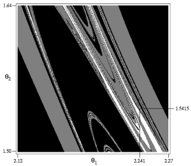
Figure 1: Fractal basin boundaries showing three possible outcomes for the binary system as a function of the initial spin alignments.

We use three methods to estimate the principle Lyapunov exponent:

Method (A) determines the full evolution matrix $L_{ij}$ from eqn. 4 and uses eqn. 6 to calculate $\lambda_{p}$. This is the most numerically intensive method as it involves integration of the 144 components of the evolution matrix $L_{ij}$ as well as the 12 components of the trajectory itself. The advantage of this method is that it yields an unambiguous computation of the stability of an orbit with no approximations.

Method (B) uses shadow trajectories and eqn. 7 with a careful rescaling of the shadow orbit. This method involves the approximation of eqn. 7, along with rescaling and the projection described by eqn. 9.

Method (C) uses eqn. 2 to evolve $\delta\vec{X}(t)$ along the reference trajectory $\vec{X}(t)$ so that a total of 24 equations are integrated and used to calculate

$$\lambda_{c}=\lim_{t\rightarrow\infty}\lim_{\delta X(0)\rightarrow 0}\frac{1}{t}\log\left(\frac{\delta X(t)}{\delta X(0)}\right).$$ (10)

This method combines the accuracy of integrating the stability equations with the approximation of projecting onto the distortion matrix as in eqn. 9.

In addition to these methods we also studied the rate of phase decoherence in the waveforms of the reference and shadow trajectories. According to Ref. njc2 , the phase difference $|\delta\Phi(t)|$ should grow as $e^{\lambda_{p}t}$. In summary, all four methods for estimating $\lambda_{p}$ use some measure $D(t)$, where $D(t)$ is equal to $\Lambda^{1/2}_{jj}(t)$, $dX(t)$, $d(t)$ or $|\delta\Phi(t)|$, depending on the method. In each case, the quantity $D(t)$ will have an initial power-law rise that is followed by exponential growth for unstable orbits.

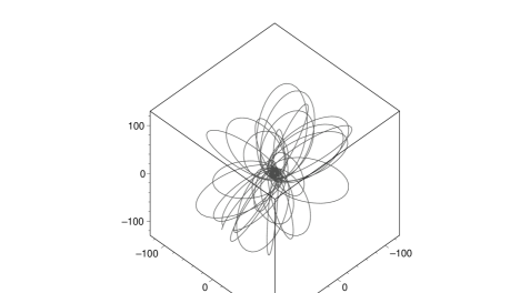
Figure 2: Trajectory taken from the fractal basin boundary of Figure 1. The axes are scaled in units of the total mass.

To illustrate the connection between the fractal structures and Lyapunov exponents, we begin by regenerating Figure 3 of Ref. jj1 in our Figure 1. The trajectories were started in the $x-y$ plane with initial conditions $({\bf x},\dot{{\bf x}})=(5.0M,0,0,0,0.45,0)$ and spin alignments $\theta_{1}$ and $\theta_{2}$ relative to the orbital angular momentum. The bodies have a $1:3$ mass ratio and spins $S_{i}=0.6m_{i}^{2}$. The trajectories were color coded according to their outcomes: Black for merger from above the $x-y$ plane, dark grey for merger from below the $x-y$ plane, white for more than 50 orbits, and light grey for escape beyond $r=1000M$. The lower panel in Figure 1 shows a detail of the fractal basin boundary, and the location of a long-lived orbit that lies close to the basin boundary. A portion of this trajectory is shown in Figure 2. The orbit has average period $T_{o}=1687M$, mean eccentricity $e=0.922$ and mean semi-major axis $a=66.7M$. Integrating the radiation reaction force along the orbit gives a decay rate of $<\!\dot{E}\!>=-1.26\times 10^{-6}$. In Figure 3 we plot $\log(D(t)/D(0))$ for this trajectory using methods A, B and C described above. All three methods yield $T_{\lambda}=11500M\sim 6.8T_{o}$ for the Lyapunov timescale, where we take an orbit to be a topological winding around the center of mass. The Lyapunov timescale is less than seven orbital periods, indicating that the motion is very chaotic.

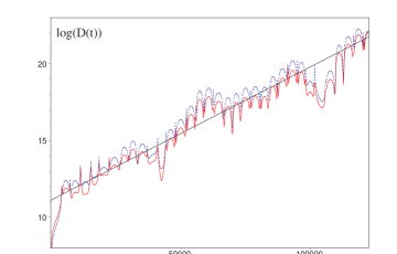
Figure 3: Determining of the principle Lyapunov exponent for the trajectory in Figure 2. The upper line uses method A, while the lower two lines (which lie over one another) use methods B and C.

Similar results were found for many other orbits taken from Figure 1. Most of the orbits near the boundaries tended to be highly eccentric ($e>0.9$), by virtue of being on the boundary and so on the cusp between merger and stability. We did find some less eccentric orbits that had positive Lyapunov exponents. For example, the trajectory with initial conditions $({\bf x},\dot{{\bf x}})=(5.5M,0,0,0,0.4,0)$, $\theta_{1}=\pi/2$, $\theta_{2}=\pi/6$, mass ratio $1:3$ and spins $S_{i}=m_{i}^{2}$ is also highly chaotic. The orbit has average period $T_{o}=275M$, mean eccentricity $e=0.59$ and mean semi-major axis $a=13.7M$. Plots of $\log(D(t)/D(0))$ are shown in Figure 4. In this case we used method $C$ and the phase divergence method to estimate $T_{\lambda}$. Both methods gave $T_{\lambda}=3080M=11.2T_{o}$, which indicates that the orbit is highly chaotic.

We found large numbers of orbits, with a range of mass ratios, spin parameters and spin alignments that had positive Lyapunov exponents. The timescale for the chaotic behaviour was often a small multiple of the orbital period.

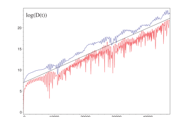
Figure 4: Determination of the principle Lyapunov exponent for the less eccentric orbit described in the text. The upper line shows $\log(d(t)/d(0))$ while the lower line shows $\log(|\delta\Phi(t)|/|\delta\Phi(0)|)$.

To further compare with Ref. ras , we took up their case of a binary with mass ratio $1:1$ and spins $S_{i}=m_{i}^{2}$, $\theta_{1}=38^{o}$, $\theta_{2}=70^{o}$. We found a positive Lyapunov exponent for $({\bf x},\dot{{\bf x}})=(5.0M,0,0,0,0.399,0)$. Therefore at least some of the equal mass binaries demonstrate chaotic orbits. As is common in chaotic systems, different trajectories came with different exponents, some of which were zero. For example, the orbit with initial conditions $({\bf x},\dot{{\bf x}})=(5.0M,0,0,0,0.428,0)$ gave $\lambda_{p}=0$. Herein lies an inherent weakness of the Lyapunov exponents themselves. They vary from orbit to orbit. A much more powerful survey of the phase space scans for chaos using fractal basin boundaries as in Figure 1.

We used four methods to determine $\lambda_{p}$, along with a battery of numerical tests, and our results have proven robust. We therefore confirm the chaos discovered in Refs. jj1 ; jj2 , contrary to the claims of Ref. ras . It should also be emphasized that the fractal basin boundary method used in Ref. jj1 is an unambiguous declaration of chaos, and alone stands as proof of chaotic dynamics njc ; mixm . Still, the Lyapunov timescales can be useful for determining the impact of chaos on the gravitational wave detection.

Now that we have confirmed that the 2PN dynamics is chaotic, we turn to the question of how significant the effect is. To this end we went to the next order in the post-Newtonian expansion and included the radiation reaction force. The effect of the radiation reaction force on the trajectory studied in Figure 4 is shown in Figure 5. Starting at an arbitrary point along the orbit, we see that the radiation reaction force drives the evolution from inspiral to plunge in roughly 5 orbits. This is comparable to the Lyapunov timescale of roughly 11 orbits. It tells us is that the chaotic behaviour seen at 2PN order is marginal when radiation reaction is included. That is, chaos is damped by dissipation, but at least for some orbits the Lyapunov timescale is comparable to the dissipation timescale. Both the instability of the orbits and the degree of damping increase as merger is approached.

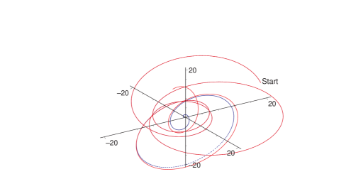
Figure 5: A detail of trajectory (solid line) showing the effect of radiation reaction (dotted line).

There is another way to show that the chaotic behaviour found in the non-dissipative 2PN dynamics does leave an imprint on the dissipative 2.5PN dynamics. The effect is illustrated in Figure 6 where trajectories with initial conditions $({\bf x},\dot{{\bf x}})=(30M,0,0,0,0.12,0)$, mass ratio $1:1$ and spins $S_{i}=0.6m_{i}^{2}$ were evolved for a range of spin-orbit alignments. The initial conditions were color coded using the same scheme as before. Despite the damping, the outcomes are intertwined in a complicated fashion. As pointed out in Ref. njc2 , with dissipation the system will not show fully fractal boundaries. However, the imprint of the underlying chaos of the conservative system is recorded in the amount of structure shown in the basin boundaries before the fractal cuts off and is rendered smooth. The detailed view in the lower panel shows that the boundaries are eventually smooth rather than fractal.

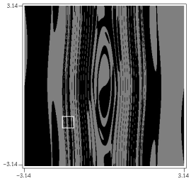
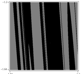
Figure 6: Basin boundaries with radiation reaction. The upper panel shows a complicated intertwining of outcomes, however the detailed view shows that the boundaries are not fractal.

It is worth comparing our results to the interesting work of Ref. ms . The authors of Ref. ms also found a positive Lyapunov exponent for spinning test particle motion around a Schwarzschild black hole. However, the light companion required an unphysically large spin many many times maximal. Here we find that the additional non-linearity from the gravitational interaction of the two bodies has introduced chaotic dynamics for physically realistic spins below maximal. We emphasize that the dynamics we study is only an approximation. We fully expect that the additional corrections at higher order in the PN expansion will augment the nonlinear behaviour and exacerbate the chaotic motion. The very difficulty in solving the two-body problem in general relativity hints that the two-body problem itself, perhaps even without the addition of spins, is fully chaotic.

In conclusion, there is chaos in the 2PN equations of motion. The chaos is damped by dissipation at 2.5PN order so that most orbits will only be mildly influenced by the complicated dynamics. What we draw from this is that matched filtering may survive as a viable technique up until the innermost orbits are reached. However, around the innermost orbits through to the plunge we will need to rely on other techniques (as already noted in Ref. scott ). Importantly, the very idea of the innermost stable circular orbit (ISCO) must be abandoned. It is telling that the most unstable motion does appear to occur in the vicinity of the homoclinic orbits. (Homoclinic orbits lie on the boundary between dynamical stability and instability us . The ISCO is a specific example of a homoclinic orbit.) The underlying chaos of the conservative dynamics means that unstable periodic orbits crowd this region of phase space. The fractal basin boundaries are a reflection of this fractal set of unstable periodic orbits. Consequently chaos can be significant for the transition to plunge, as well as for the final orbits.

References

- (1) S. Suzuki & K. Maeda, Phys. Rev. D55, 4848 (1997).
- (2) J. Levin, Phys. Rev. Lett. 84, 3515 (2000).
- (3) N. J. Cornish, Phys. Rev. D64, 084011 (2001).
- (4) J. Levin, Preprint gr-qc/0010100 (2001).
- (5) N. J. Cornish, Phys. Rev. Lett. 85, 3980 (2000).
- (6) S. Hughes, Phys.Rev.Lett. 85 5480 (2000).
- (7) J.D. Schnittman & F.A. Rasio, Phys. Rev. Lett. 87, 121101 (2001).
- (8) L. Kidder, Phys. Rev. D52, 821 (1995).
- (9) E. Poisson, Phys. Rev. D57, 5287 (1998).
- (10) H. Tagoshi, A. Ohashi & B. Owen, Phys. Rev. D63, 044006 (2001).
- (11) C.P. Dettmann, N. E. Frankel & N.J. Cornish, Phys. Rev. D.50 R618 (1994).
- (12) N.J. Cornish & J.J. Levin, Phys. Rev. Lett. 78 998 (1997); Phys. Rev. D.55 7489 (1997).
- (13) J. Levin, R. O’Reilly, & E.J. Copeland, Phys. Rev. D62, 024023 (2000).