Bulk Fermion Stars with New Dimensions

Abstract

Many efforts have been devoted to the studies of the phenomenology in particle physics with extra dimensions. We propose degenerate fermion stars with extra dimensions and study what features characterized by the size of extra dimensions should appear in its structure. We find that Kaluza-Klein excited modes arise for the larger scale of extra dimensions and examine the conditions on which different layers should be caused in the inside of the stars. We expound how the extra dimensions affect on physical quantities.

Graduate School of Science and Engineering, Yamaguchi University,
Yoshida,Yamaguchi-shi,Yamaguchi 753-8512, Japan

1 Introduction

Recently, physics dealing with higher dimensions has been investigated [1, 2, 3]. Considering extra dimensions in Grand Unified Theories (GUTs), it is suggested that forces could be unified at low energy scale. The first string realization of low scale gravity models was given in [4]. In this model, only gravity acts on extra dimensions, while the standard particles on the brane have no effects. On the other hand, a low GUT scale has been obtained in [2], in which all the gauge particles and gravity feel extra dimensions.

In this paper, we consider that gravity and bulk matters have effects on extra dimensions and study how the extra spaces influence the bulk matters through the gravity. To investigate the influence, we propose a self-gravitational system, namely star, which is made of degenerate Dirac fermions with the extra dimensions.

When extra dimensions are compactified, Kaluza-Klein (K-K) excited modes arise. In the present study, taking account of the K-K modes, we consider the fermion star with extra dimensions and indicate that the excited modes affect the inside of star. After asking for the maximum mass and the radius by use of numerical calculation, we will make it clear what the interior structure of star should be.

We begin in Sec. 2 with five dimensional theory and extend the argument into the $(4+d)$ dimensional one in Sec. 3. Sec. 4 describes the star in six dimensions where extra dimensions are anisotropic. Conclusion and discussion are summarized in Sec. 5.

2 (4+1) dimensional Bulk Fermion Star

2.1 Matter

2.1.1 (3+1) dimensions

In the four dimensional theory, the thermodynamic potential of a fermion gas with mass $m$ and half spin is

$$\Omega_{4}=-2\frac{1}{\beta}V\int\frac{d^{3}\textbf{p}}{(2\pi)^{3}}\left[\ln\left(1+e^{-\beta(\sqrt{\textbf{p}^{2}+m^{2}}-\mu)}\right)+(\mu\leftrightarrow-\mu)\right],$$ (1)

where we put subscript to emphasize that it stands for a four dimensional quantity. We will restrict our system to degenerate fermion gas and take the zero temperature limit. Then, the thermodynamic potential becomes

$$\Omega_{4}(m)\equiv\left\{\begin{array}[]{@{\,}ll}-V\frac{m^{4}}{24\pi^{2}}\left[\frac{\mu}{m}\sqrt{\frac{\mu^{2}}{m^{2}}-1}\left(2\frac{\mu^{2}}{m^{2}}-5\right)+3\ln\left|\frac{\mu}{m}+\sqrt{\frac{\mu^{2}}{m^{2}}-1}\right|\right]&(m<\mu)\\ 0&(m\geqq\mu)\end{array}.\right.$$ (2)

Thermodynamical quantities will follow from Eq. (2).

2.1.2 (4+1) dimensions

We will extend our argument into the five dimensional theory. Here we suppose that the fifith dimension is compactified into $S^{1}$ with a radius $b$, $b$ is not so large. We impose the periodic boundary condition on a wave function in the fifth dimension:

$$\psi(x_{5})\approx{e^{ip_{5}\cdot x_{5}}}~{},$$ (3)

$$\psi(x_{5}+2\pi{b})\sim\psi(x_{5})~{},$$ (4)

with the fifth coordinate $x_{5}$ and momentum $p_{5}$ . Eq.(3) and (4) give

$$p_{5}=\frac{n}{b}\ \ \ \mbox{($n$: integer)}~{}.$$ (5)

Therefore the relativistic energy involving the fifth dimension is

$$E_{5} = \sqrt{{\bf p}^{2}+\left(\frac{n}{b}\right)^{2}+m^{2}}$$ (6)

$$= \sqrt{{\bf p}^{2}+M^{2}}~{},$$ (7)

where

$$M^{2}\equiv\left(\frac{n}{b}\right)^{2}+m^{2}~{}.$$ (8)

Using Eq. (7), the thermodynamic potential of the fermion gas with mass $m$ and half spin in the (4+1) dimensional space-time is

$$\Omega_{5}=-2\frac{1}{\beta}V_{4}\int\frac{d^{4}\textbf{p}}{(2\pi)^{4}}\left[\ln\left(1+e^{-\beta(\sqrt{\textbf{p}^{2}+M^{2}}-\mu)}\right)+(\mu\leftrightarrow-\mu)\right]~{}.$$ (9)

If the integral over the fifth dimensional momentum is turned into the sum over quantum number $n$ :

$$\int dp_{5}\to\frac{1}{b}\sum_{n}~{},$$ (10)

in addition,

$$V_{4}=2\pi{b}V~{},$$ (11)

then the thermodynamic potential is

$$\Omega_{5} = -2\frac{1}{\beta}V\sum_{n}\int\frac{d^{3}\textbf{p}}{(2\pi)^{3}}\left[\ln\left(1+e^{-\beta(\sqrt{\textbf{p}^{2}+\frac{n^{2}}{b^{2}}+m^{2}}-\mu)}\right)+(\mu\leftrightarrow-\mu)\right]$$ (12)

$$= \sum_{n}\Omega_{4}\left(\sqrt{m^{2}+\frac{n^{2}}{b^{2}}}\right)=\sum_{n}\Omega_{4}(M)~{}.$$

(Unless $n=0$, the K-K modes become effective.) As well as the previous subsection, we will deal with the degenerate fermion gas and low temperature near to zero. The thermodynamic potential, therefore, becomes

$$\Omega_{5}(V,\mu,b)=\left\{\begin{array}[]{@{\,}ll}-Vb^{-4}f(\mu{b},mb)&(\mu>M)\\ 0&(\mu\leqq{M})\end{array}~{},\right.$$ (13)

where

$$f\equiv\sum_{M<\mu}\frac{(Mb)^{4}}{24\pi^{2}}\left\{\frac{\mu{b}}{Mb}\left(2\left(\frac{\mu{b}}{Mb}\right)^{2}-5\right)\sqrt{\left(\frac{\mu{b}}{Mb}\right)^{2}-1}+3\ln\left|\sqrt{\left(\frac{\mu{b}}{Mb}\right)^{2}-1}+\frac{\mu{b}}{Mb}\right|\right\}~{}.$$ (14)

From Eq. (13), thermodynamical quantities are as follows:

$$P=-\frac{1}{2\pi{b}}\frac{\partial\Omega_{5}}{\partial{V}}=-\frac{1}{2\pi{b}}\frac{\Omega_{5}}{V}=\frac{1}{2\pi{b}}\frac{1}{b^{4}}f~{},$$ (15)

$$P_{5}=-\frac{1}{2\pi{V}}\frac{\partial{\Omega_{5}}}{\partial{b}}=\frac{1}{2\pi{b}}\frac{1}{b^{4}}\left(x\frac{\partial{f}}{\partial{x}}+y\frac{\partial{f}}{\partial{y}}-4f\right)~{},$$ (16)

$$\rho=\frac{U}{V_{4}}=\frac{1}{2\pi{b}}\frac{1}{b^{4}}\left(x\frac{\partial{f}}{\partial{x}}-f\right)~{},$$ (17)

where $P_{5}$ is the pressure in the fifth dimension, and we put  $x=\mu{b}$ and $y=mb$.

2.2 Space-Time

The line element can be written as

$$ds^{2}=e^{-\Phi}\left[-e^{-2\delta}\Delta{dt^{2}}+\frac{dr^{2}}{\Delta}+r^{2}(d\theta^{2}+\sin^{2}\theta{d\varphi^{2}})\right]+b_{0}^{2}e^{2\Phi}{d\chi}^{2}~{}.$$ (18)

Here we regard $\Delta$, $\delta$, and $\Phi$ ($b=b_{0}e^{\Phi}$) as functions depending only on $r$, which is the distance from the origin. The energy-momentum tensor is

$$T^{\mu}\!_{\nu}=diag.(-\rho,P,P,P,P_{5})~{}.$$ (19)

We suppose isotropic pressure in the space of three dimensions and represent the fifth dimensional pressure as $P_{5}$. The equation of conservation is

$$\nabla_{\mu}T^{\mu{r}}=0~{}.$$ (20)

Eq.(20) gives the condition that the chemical potential $\mu$ satisfies

$$\mu{b}=\frac{e^{\frac{3}{2}\Phi+\delta}}{\sqrt{\Delta}}\mu_{0}b_{0}~{},$$ (21)

where $\mu$ depends on $r$, and $\mu_{0}$ and $b_{0}$ are the value of $\mu$ and $b$ when $r$ is close to zero respectively.

2.3 Equations

We are just deriving the Einstein equations. Before that, we will rewrite Eq. (14) for convenience. Putting

$$x=\mu{b},~{}~{}~{}y=mb$$

reduces Eq. (14) to

$$f(x,y) = {\sum_{n}}^{\prime}\frac{(y^{2}+n^{2})^{2}}{24\pi^{2}}\left[\frac{x}{\sqrt{y^{2}+n^{2}}}\sqrt{\frac{x^{2}}{y^{2}+n^{2}}-1}\left(2\frac{x^{2}}{y^{2}+n^{2}}-5\right)\right.$$ (22)

$$\left.+3\ln\left|\frac{x}{\sqrt{y^{2}+n^{2}}}+\sqrt{\frac{x^{2}}{y^{2}+n^{2}}-1}\right|\right]$$

$$= {\sum_{n}}^{\prime}\tilde{f}(x,y)\ \ \ \ \ \ \ (\sqrt{x^{2}-y^{2}}>|n|)~{},$$

where the sum over $n$ is done unless $|n|$ exceeds $\sqrt{x^{2}-y^{2}}$ . (To remark this, we put prime on a sum symbol.) In addition, we put

$$Y=\sqrt{y^{2}+n^{2}}~{}.$$ (23)

The leading formulae lead to the Einstein equations:

$$\frac{{\tilde{M}_{\star}}^{\prime}}{\tilde{r}^{2}}-\frac{3}{8}\tilde{\Delta}(\Phi^{\prime})^{2}=4\pi\frac{1}{m^{4}b^{4}_{0}}e^{-6\Phi}{\sum}^{\prime}\left(x\frac{\partial\tilde{f}}{\partial{x}}-\tilde{f}\right)~{},$$ (24)

$$\frac{1}{\tilde{r}}\delta^{\prime}+\frac{3}{4}(\Phi^{\prime})^{2}=-4\pi\frac{1}{m^{4}b^{4}_{0}}\frac{e^{-6\Phi}}{\tilde{\Delta}}{\sum}^{\prime}\left(x\frac{\partial\tilde{f}}{\partial{x}}\right)~{},$$ (25)

$$\Phi^{\prime\prime}+\left(\frac{\tilde{\Delta}^{\prime}}{\tilde{\Delta}}-\delta^{\prime}+\frac{2}{\tilde{r}}\right)\Phi^{\prime} = -\frac{8\pi}{3}\frac{1}{m^{4}b^{4}_{0}}\frac{e^{-6\Phi}}{\tilde{\Delta}}{\sum}^{\prime}\left(\frac{3Y^{2}-2y^{2}}{Y^{2}}x\frac{\partial\tilde{f}}{\partial{x}}\right.$$ (26)

$$\left.-\frac{12Y^{2}-8y^{2}}{Y^{2}}\tilde{f}\right)~{},$$

where

$$\tilde{M}_{\star} = \sqrt{G_{4}m^{2}}G_{4}mM_{\star}~{},$$ (27)

$$\tilde{r} = \sqrt{G_{4}m^{4}}r~{},$$ (28)

$$\tilde{\Delta} = 1-\frac{2\tilde{M}_{\star}}{\tilde{r}}~{}.$$ (29)

In the above equations, we define a usual Newtonian constant $G_{4}$ as

$$G_{4}\equiv\frac{G_{5}}{2\pi{b_{0}}}~{}.$$ (30)

Here $G_{5}$ stands for the Newtonian constant in the fifth dimension. $M_{\star}$ is the mass interior to radius $r$. A prime means derivative with respect to $\tilde{r}$. We can solve these equations numerically. In the next section, we will show the result.

2.4 Numerical Results

We will exhibit the relationship between the mass and the central density in fermion stars in Fig. 1, and between the mass and the radius in Fig. 2, where $\bar{M}=(G_{4}^{3/2}m^{2})^{-1}=\frac{M_{P}^{3}}{m^{2}}$ with the Planck mass $M_{P}$ and $\bar{R}=(G_{4}^{1/2}m^{2})^{-1}=\frac{\bar{\lambda}^{2}}{l_{P}}$ with the Planck length $l_{P}$ and the Compton wave length $\bar{\lambda}$. These results indicate that as the size of the extra space becomes larger, the maximum mass becomes smaller. Furthermore, it is remarkable that two maximum points appear when $mb_{0}=3.0,4.0$.

Fig. 1: Plots of the mass $M$ of the fermion stars versus its central density $\rho_{0(4)}$ for the various scales of the extra dimension. The dashed line corresponds to $mb_{0}\approx 0$. The dot-dashed line corresponds to $mb_{0}=1.0$, the two dot-dashed line to $mb_{0}=2.0$, the three to $mb_{0}=3.0$, the four to $mb_{0}=4.0$.

Fig. 2: Plots of the mass $M$ of the fermion stars versus its radius $R$ for the various scales of the extra dimension. The correspondence between the dashed lines and the scales of the fifth dimension is the same as Fig. 1.

Fig. 3 exhibits the interior structure of the stars having the maximum mass. From Fig. 3, we find that the excited modes have effects in the core of the stars as the size of the fifth dimension grows. We have two solutions with the maximum mass in the case of $mb_{0}=3.0,4.0$. For $mb_{0}=3.0$, one of them is a larger star and the other is a smaller one than the star with the maximum mass for $mb_{0}=2.0$ respectively.

The central density of the larger star for $mb_{0}=3.0$ is lower than that of the star for $mb_{0}=2.0$, while the central density of the smaller star for $mb_{0}=3.0$ is higher than that of the star for $mb_{0}=2.0$, as Fig. 1 shows. In the latter solution, a higher excited mode ($n$=2) is caused mainly in the center of stars and a lower mode ($n$=1) in the vast region including the core. Proceeding to $mb_{0}=4.0$, this inclination appears more remarkably.

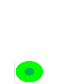
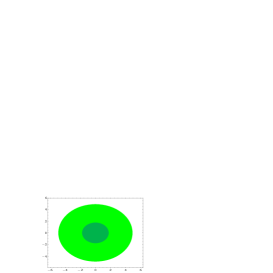
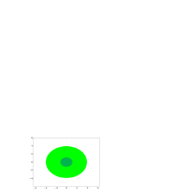
$mb_{0}=4.0$               $mb_{0}=3.0$                                                                                                                          $mb_{0}=2.0$                                                                                                                          $mb_{0}=1.0$

Fig. 3: The sequence of the fermion stars with the increase of the size of the extra dimension. In the darkest disk, $n=2$ mode is most effective. In the middle one, $n=1$ mode is effective. In the pale disk, there is no excited mode.

3 (4+d) dimensional Bulk Fermion Stars

We will extend the preceding argument into the $(4+d)$ dimensional theory.

3.1 Matter

3.1.1 (4+d) dimensions

We suppose that the extra dimensions are compactified into $T^{d}$ with a radius $b$, $b$ is not so large. Each of the momenta in the extra dimensions is

$$p_{ex}^{i}=\frac{n_{i}}{b}\qquad(i=1,2,\dots,d)~{}.$$ (31)

Therefore, considering the $d$ momenta, the relativistic energy is

$$E_{(4+d)} = \sqrt{{\bf p}^{2}+\sum_{i}\left(\frac{n_{i}}{b}\right)^{2}+m^{2}}$$ (32)

$$= \sqrt{{\bf p}^{2}+M_{(4+d)}^{2}}~{},$$ (33)

where

$$M_{(4+d)}=\sqrt{\sum_{i}\left(\frac{n_{i}}{b}\right)^{2}+m^{2}}~{}.$$ (34)

Using Eq. (32), changing the integral over the extra spatial momenta into the sum over quantum number $n_{i}$ and holding the replacement $V_{(3+d)}\to\left(2\pi b\right)^{d}V$, the $(4+d)$ dimensional thermodynamic potential for a fermion gas with mass $m$ and half spin is

$$\Omega_{(4+d)}=\frac{2^{[\frac{4+d}{2}]}}{4}\sum_{n_{1}}\sum_{n_{2}}\cdots\sum_{n_{d}}\Omega_{4}\left(\sqrt{m^{2}+\frac{{\bf n}^{2}}{b^{2}}}\right)~{},$$ (35)

where

$${\bf n}^{2}=\sum_{i=1}^{d}n_{i}^{2}~{}.$$ (36)

(Each $n_{i}$ is an integer. Unless ${\bf{n}}^{2}=0$ , the K-K modes become effective.) $\Omega_{4}$ stands for a four dimensional one. We will restrict our system to degenerate fermion gas and take the zero temperature limit. Therefore, with the help of Eq. (13), the thermodynamic potential becomes

$$\Omega_{(4+d)}(V,\mu,b)=\left\{\begin{array}[]{@{\,}ll}-V{b^{-4}}f_{(4+d)}\left(\mu b,mb\right)&(\mu>M_{(4+d)})\\ 0&(\mu\leqq M_{(4+d)})\end{array}~{},\right.$$ (37)

where

$$f_{(4+d)} \equiv \sum\dots\sum\frac{2^{[\frac{4+d}{2}]}}{4}\frac{(M_{(4+d)}b)^{4}}{24\pi^{2}}\left[\frac{\mu b}{M_{(4+d)}b}\sqrt{\frac{(\mu b)^{2}}{(M_{(4+d)}b)^{2}}-1}\left(2\frac{(\mu b)^{2}}{(M_{(4+d)}b)^{2}}-5\right)\right.$$ (38)

$$\qquad\qquad\qquad\qquad\qquad\quad\quad\left.+3\ln\left|\frac{\mu b}{M_{(4+d)}b}+\sqrt{\frac{(\mu b)^{2}}{(M_{(4+d)}b)^{2}}-1}\right|\right]~{}.$$

The sum over $n_{1},n_{2},\cdots,n_{d}$ are done unless $M_{(4+d)}$ exceeds $\mu$. From Eq. (37), thermodynamical quantities are as follows:

$$P=-\frac{1}{(2\pi b)^{d}}\left(\frac{\partial\Omega_{(4+d)}}{\partial V}\right)_{\mu,b}=\frac{1}{(2\pi b)^{d}}\frac{1}{b^{4}}f_{(4+d)}~{},$$ (39)

$$P_{ex}=-\frac{1}{(2\pi b)^{d}V}\frac{1}{d}b\left(\frac{\partial\Omega_{(4+d)}}{\partial b}\right)_{V,\,\mu}=\frac{1}{(2\pi b)^{d}}\frac{1}{d}\frac{1}{b^{4}}\left(x\frac{\partial f_{(4+d)}}{\partial x}+y\frac{\partial f_{(4+d)}}{\partial y}-4f_{(4+d)}\right)~{},$$ (40)

$$\rho=\frac{U}{V_{(4+d)}}=\frac{1}{{(2\pi b)}^{d}}\frac{1}{b^{4}}\left(x\frac{\partial f_{(4+d)}}{\partial x}-f_{(4+d)}\right)~{},$$ (41)

where $P_{ex}$ is the pressure in each extra dimension, and we put  $x=\mu{b}$ and $y=mb$.

3.2 Space-Time

We take the line element to be of the form

$$ds^{2}=e^{-d\Phi}\left[-e^{-2\delta}\Delta{dt^{2}}+\frac{dr^{2}}{\Delta}+r^{2}(d\theta^{2}+\sin^{2}\theta{d\varphi^{2}})\right]+b_{0}^{2}e^{2\Phi}\sum_{i=1}^{d}{d\chi_{i}}^{2}~{},$$ (42)

where we regard $\Delta$, $\delta$, and $\Phi$ ($b=b_{0}e^{\Phi}$) as functions depending only on $r$, the distance from the origin. The energy-momentum tensor is

$$T^{\mu}\!_{\nu}=diag.(-\rho,P,P,P,P_{ex},\cdots,P_{ex})~{}.$$ (43)

We suppose isotropic pressure in the space of three dimensions and represent the extra dimensional pressure as $P_{ex}$. The equation of conservation is

$$\nabla_{\mu}T^{\mu{r}}=0~{}.$$ (44)

From Eq. (44), we find the chemical potential $\mu$ satisfies

$$\mu{b}=\frac{e^{\frac{d+2}{2}\Phi+\delta}}{\sqrt{\Delta}}\mu_{0}b_{0}~{},$$ (45)

where $\mu$ depends on $r$, and $\mu_{0}$ and $b_{0}$ are the values for $\mu$ and $b$ at $r=0$ respectively.

3.3 Equations

We are just deriving the Einstein equations. As well as the previous section, we will rewrite Eq. (38) for convenience. Putting $x=\mu b$ and $y=mb$ reduces Eq. (38) to

$$f_{(4+d)}\left(x,y\right) = \frac{2^{[\frac{d+4}{2}]}}{4}{\sum_{{\bf n}}}^{{}^{\prime}}\frac{\left(y^{2}+{\bf n}^{2}\right)^{2}}{24\pi^{2}}\left[\frac{x}{\sqrt{y^{2}+{\bf n}^{2}}}\sqrt{\frac{x^{2}}{y^{2}+{\bf n}^{2}}-1}\left(2\frac{x^{2}}{y^{2}+{\bf n}^{2}}-5\right)\right.$$ (46)

$$\left.+3\ln\left|\frac{x}{\sqrt{y^{2}+{\bf n}^{2}}}+\sqrt{\frac{x^{2}}{y^{2}+{\bf n}^{2}}-1}\right|\right]$$

$$= {\sum_{{\bf n}}}^{{}^{\prime}}\tilde{f}_{(4+d)}\left(x,y\right)\ \ \ \ \ \ \ (x^{2}-y^{2}>\bf{n}^{2})~{},$$ (47)

where

$${\bf n}^{2}=\sum_{i=1}^{d}{n_{i}}^{2}~{}.$$ (48)

The sum over ${\bf n}$ is done unless ${\bf n}^{2}$ exceeds $x^{2}-y^{2}$ . (To remark this, we put prime on a sum symbol.) In addition, we put

$$Y=\sqrt{y^{2}+{\bf n}^{2}}~{}.$$ (49)

The leading formulae lead to the Einstein equations:

$$\frac{\tilde{M}_{\star}^{\prime}}{\tilde{r}^{2}}-\frac{d(d+2)}{8}\tilde{\Delta}\left(\Phi^{\prime}\right)^{2}=4\pi\frac{1}{m^{4}b_{0}^{4}}e^{-2(d+2)\Phi}{\sum}^{\prime}\left(x\frac{\partial\tilde{f}_{(4+d)}}{\partial x}-\tilde{f}_{(4+d)}\right)~{},$$ (50)

$$\frac{1}{\tilde{r}}\delta^{\prime}+\frac{d(d+2)}{4}\left(\Phi^{\prime}\right)^{2}=-4\pi\frac{1}{m^{4}b_{0}^{4}}\frac{e^{-2(d+2)\Phi}}{\tilde{\Delta}}{\sum}^{\prime}\left(x\frac{\partial\tilde{f}_{(4+d)}}{\partial x}\right)~{},$$ (51)

$$\Phi^{\prime\prime}+\left(\frac{\tilde{\Delta}^{\prime}}{\tilde{\Delta}}-\delta^{\prime}+\frac{2}{\tilde{r}}\right)\Phi^{\prime} = -\frac{8\pi}{d(d+2)}\frac{1}{m^{4}b_{0}^{4}}\frac{e^{-2(d+2)\Phi}}{\tilde{\Delta}}$$ (52)

$$\times{\sum}^{\prime}\left(\frac{(d+2)Y^{2}-2y^{2}}{Y^{2}}x\frac{\partial\tilde{f}_{(4+d)}}{\partial x}-\frac{4(d+2)Y^{2}-8y^{2}}{Y^{2}}\tilde{f}_{(4+d)}\right)~{},$$

where $\tilde{M_{\star}}(\tilde{r})=\sqrt{G_{4}m^{2}}{G_{4}mM_{\star}}$, $\tilde{r}=\sqrt{G_{4}m^{4}}r$ and $\tilde{\Delta}=1-\frac{2\tilde{M}_{\star}}{\tilde{r}}$. Here we define a usual Newtonian constant $G_{4}$ as

$$G_{4}\equiv\frac{G_{(4+d)}}{(2\pi{b_{0}})^{d}}~{},$$ (53)

in which $G_{(4+d)}$ stands for the Newtonian constant in the $(4+d)$ dimensions. $M_{\star}$ is the mass interior to radius $r$. A prime means derivative with respect to $\tilde{r}$. We can solve these numerically. In the next section, we will show one of the results.

3.4 Numerical Results

We will exhibit the relationship between the mass and the central density in fermion stars in Fig. 4, and between the mass and the radius in Fig. 5 in six dimensions, where $\bar{M}=(G_{4}^{3/2}m^{2})^{-1}=\frac{M_{P}^{3}}{m^{2}}$ with the Planck mass $M_{P}$ and $\bar{R}=(G_{4}^{1/2}m^{2})^{-1}=\frac{\bar{\lambda}^{2}}{l_{P}}$ with the Planck length $l_{P}$ and the Compton wave length $\bar{\lambda}$. It turns out that as the size of the extra space becomes larger, the maximum mass becomes smaller. Furthermore, it is remarkable that two maximum points appear when $mb_{0}=5.0,6.0,7.0$. For $mb_{0}=5.0,6.0$, one of them is a larger star than that for $mb_{0}=4.0$ and its central density is lower. In this solution, only the lowest mode (${\bf n}^{2}=1$) is caused in the center of stars. While the other is a smaller star and its central density is higher. In this solution, higher excited modes (${\bf n}^{2}=4,5$) are caused mainly in the center of stars and lower modes (${\bf n}^{2}=1,2$) in the vast region including the core. Proceeding to $mb_{0}=7.0$, this inclination appears more remarkably. We can draw the interior structure of the stars having the maximum mass, but we omit them here. As for seven, eight and more dimensional theories, the maximum mass becomes smaller with the increase of the scale of extra dimensions, which is similar to six one, but the maximum point is one and only one. In these solutions, the lowest mode (${\bf n}^{2}=1$) is caused in the center of stars.

Fig. 4: Plots of the mass $M$ of the fermion stars versus its central density $\rho_{0(4)}$ for the various scales of the extra dimensions. The solid line corresponds to $mb_{0}=1.0$. The dashed line corresponds to $mb_{0}=2.0$, the dot-dashed line to $mb_{0}=3.0$, the two dot-dashed line to $mb_{0}=4.0$, the three to $mb_{0}=5.0$, the four to $mb_{0}=6.0$, the broken line to $mb_{0}=7.0$.

Fig. 5: Plots of the mass $M$ of the fermion stars versus its radius $R$ for the various scales of the extra dimensions. The correspondence between the lines and the scales of the extra dimensions is the same as Fig. 4.

4 Anisotropic (4+2) dimensional Bulk Fermion Star

We consider the six dimensional theory. The extra dimensions are compactified into $T^{2}$. Unlike the previous sections, We suppose that the scale of the compactified radius in the extra dimensions is different from each other.

4.1 Matter

4.1.1 Anisotropic (4+2) dimensions

We consider that the compactified radius in the fifith and sixth dimension is $b_{1}$ and $b_{2}$ , respectively. Both $b_{1}$ and $b_{2}$ are not so large. Each of the momenta in the extra dimensions is

$$p_{ex}^{1} = \frac{n_{1}}{b_{1}}\ \ \ \mbox{($n_{1}$: integer)}~{},$$ (54)

$$p_{ex}^{2} = \frac{n_{2}}{b_{2}}\ \ \ \mbox{($n_{2}$: integer)}~{}.$$ (55)

Therefore the relativistic energy involving the fifth and sixth dimension is

$$E_{6}=\sqrt{{\bf p}^{2}+(\frac{n_{1}}{b_{1}})^{2}+(\frac{n_{2}}{b_{2}})^{2}+m^{2}}\\ =\sqrt{\textbf{p}^{2}+M_{6}^{2}}~{},$$ (56)

where

$$M_{6}\equiv\sqrt{\frac{{n_{1}}^{2}}{{b_{1}}^{2}}+\frac{{n_{2}}^{2}}{{b_{2}}^{2}}+m^{2}}~{}.$$ (57)

Then, the thermodynamic potential for a fermion gas with mass $m$ and half spin is

$$\Omega_{6}=2\sum_{n_{1}}\sum_{n_{2}}\Omega_{4}\left(\sqrt{\frac{{n_{1}}^{2}}{{b_{1}}^{2}}+\frac{{n_{2}}^{2}}{{b_{2}}^{2}}+m^{2}}\right)~{}.$$ (58)

( Unless $n_{1}=n_{2}=0$, the K-K modes become effective.) $\Omega_{4}$ stands for a four dimensional one. As well as the previous sections, we will deal with the degenerate fermion gas and take the zero temperature limit. Therefore, the thermodynamic potential becomes

$$\Omega_{6}(V,\mu,\bar{b},\gamma)=\left\{\begin{array}[]{@{\,}ll}-V{\bar{b}^{-4}}f_{6}\left(\mu\bar{b},m\bar{b},\gamma\right)=-V{\bar{b}^{-4}}f_{6}\left(\bar{x},\bar{y},\gamma\right)&(\mu>M_{6})\\ 0&(\mu\leq M_{6})\end{array}~{},\right.$$ (59)

where $\bar{b}\equiv\sqrt{b_{1}b_{2}},~{}\gamma\equiv b_{2}/b_{1},~{}\bar{x}\equiv\mu\bar{b},~{}\bar{y}\equiv m\bar{b}$, and

$$f_{6} \equiv 2\sum\sum\frac{(M_{6}\bar{b})^{4}}{24\pi^{2}}\left[\frac{\mu\bar{b}}{M_{6}\bar{b}}\sqrt{\frac{(\mu\bar{b})^{2}}{(M_{6}\bar{b})^{2}}-1}\left(2\frac{(\mu\bar{b})^{2}}{(M_{6}\bar{b})^{2}}-5\right)\right.$$ (60)

$$\qquad\qquad\qquad\quad\quad\left.+3\ln\left|\frac{\mu\bar{b}}{M_{6}\bar{b}}+\sqrt{\frac{(\mu\bar{b})^{2}}{(M_{6}\bar{b})^{2}}-1}\right|\right]~{}.$$

The sum over $n_{1},n_{2}$ are done unless $M_{6}$ exceeds $\mu$. From Eq. (59), thermodynamical quantities are as follows:

$$P=-\frac{1}{{(2\pi b_{1})}{(2\pi b_{2})}}\left(\frac{\partial\Omega_{6}}{\partial V}\right)_{\mu,\bar{b},\gamma}=\frac{1}{{(2\pi\bar{b})}^{2}}\frac{1}{\bar{b}^{4}}f_{6}~{},$$ (61)

$$P_{5}=-\frac{1}{(2\pi)(2\pi b_{2})V}\left(\frac{\partial\Omega_{6}}{\partial b_{1}}\right)_{V,\,\mu}=\frac{1}{{(2\pi\bar{b})}^{2}}\frac{1}{2}\frac{1}{\bar{b}^{4}}\left(\bar{x}\frac{\partial f_{6}}{\partial\bar{x}}+\bar{y}\frac{\partial f_{6}}{\partial\bar{y}}-4f_{6}-2\gamma\frac{\partial f_{6}}{\partial\gamma}\right)~{},$$ (62)

$$P_{6}=-\frac{1}{(2\pi)(2\pi b_{1})V}\left(\frac{\partial\Omega_{6}}{\partial b_{2}}\right)_{V,\,\mu}=\frac{1}{{(2\pi\bar{b})}^{2}}\frac{1}{2}\frac{1}{\bar{b}^{4}}\left(\bar{x}\frac{\partial f_{6}}{\partial\bar{x}}+\bar{y}\frac{\partial f_{6}}{\partial\bar{y}}-4f_{6}+2\gamma\frac{\partial f_{6}}{\partial\gamma}\right)~{},$$ (63)

$$\rho=\frac{U}{V_{6}}=\frac{U}{{(2\pi\bar{b})}^{2}V}=\frac{1}{{(2\pi\bar{b})}^{2}}\frac{1}{\bar{b}^{4}}\left(\bar{x}\frac{\partial f_{6}}{\partial\bar{x}}-f_{6}\right)~{},$$ (64)

where $P_{5}$ and $P_{6}$ are the pressure in the fifth and sixth dimension, respectively, and we put  $\bar{x}=\mu\bar{b}$ and $\bar{y}=m\bar{b}$.

4.2 Space-Time

The line element can be written as

$$ds^{2}=e^{-2\Phi}\left[-e^{-2\delta}\Delta dt^{2}+\frac{dr^{2}}{\Delta}+r^{2}\left(d\theta^{2}+\sin^{2}\theta d\varphi^{2}\right)\right]+b_{1}^{2}d\chi_{1}^{2}+b_{2}^{2}d\chi_{2}^{2}~{}.$$ (65)

Here we regard $\Delta$, $\delta$, $\Phi$, $b_{1}$ and $b_{2}$ as functions depending only on $r$, the distance from the origin. The energy-momentum tensor is

$$T^{\mu}\!_{\nu}=diag.\left(-\rho,P,P,P,P_{5},P_{6}\right)~{}.$$ (66)

We suppose isotropic pressure in the space of three dimensions and represent the fifth dimensional pressure as $P_{5}$ and the sixth one as $P_{6}$. The equation of conservation $\nabla_{\mu}T^{\mu\nu}=0$ gives the condition that the chemical potential $\mu$ satisfies

$$\mu\bar{b}=\frac{e^{2\Phi+\delta}}{\sqrt{\Delta}}\mu_{0}\bar{b}_{0}~{},$$ (67)

where $\mu$ depends on $r$, and $\mu_{0}$ and $\bar{b}_{0}$ are the value of $\mu$ and $\bar{b}$ at $r=0$ respectively.

4.3 Equations

We are just deriving the Einstein equations. As well as the previous sections, we will rewrite Eq. (60) for convenience. If we put  $\bar{b}=\bar{b}_{0}e^{\Phi(r)},~{}\gamma=b_{2}/b_{1}=e^{\phi(r)},~{}\bar{x}=\mu\bar{b}$  and  $\bar{y}=m\bar{b}$,  Eq. (60) is reduced to

$$f_{6}\left(\bar{x},\bar{y},\gamma\right) = 2{\sum_{n_{1}}}^{{}^{\prime}}{\sum_{n_{2}}}^{{}^{\prime}}\frac{Y^{4}}{24\pi^{2}}\left[\frac{\bar{x}}{Y}\sqrt{\frac{{\bar{x}}^{2}}{Y^{2}}-1}\left(2\frac{{\bar{x}}^{2}}{Y^{2}}-5\right)+3\ln\left|\frac{\bar{x}}{Y}+\sqrt{\frac{{\bar{x}}^{2}}{Y^{2}}-1}\right|\right]\qquad\qquad$$ (68)

$$= {\sum_{n_{1}}}^{{}^{\prime}}{\sum_{n_{2}}}^{{}^{\prime}}\tilde{f_{6}}\left(\bar{x},\bar{y},\gamma\right)\ \ \ \ \ \ \ (\bar{x}^{2}-\bar{y}^{2}>{n_{1}}^{2}\gamma+{n_{2}}^{2}\gamma^{-1})~{},$$ (69)

where the sums over $n_{1}$ and $n_{2}$ are done unless ${n_{1}}^{2}\gamma+{n_{2}}^{2}\gamma^{-1}$ exceeds $\bar{x}^{2}-\bar{y}^{2}$ . (To remark this, we put prime on a sum symbol.) In addition, we put

$$Y=\sqrt{{\bar{y}}^{2}+{n_{1}}^{2}\gamma+{n_{2}}^{2}\gamma^{-1}}~{}.$$ (70)

The leading formulae lead to the Einstein equations :

$$\frac{\tilde{M}_{\star}^{\prime}}{\tilde{r}^{2}}-\tilde{\Delta}\left(\Phi^{\prime}\right)^{2}-\frac{1}{8}\tilde{\Delta}\left(\phi^{\prime}\right)^{2}=4\pi\frac{1}{m^{4}{\bar{b_{0}}}^{4}}e^{-8\Phi}{\sum_{n_{1}}}^{{}^{\prime}}{\sum_{n_{2}}}^{{}^{\prime}}\left(\bar{x}\frac{\partial\tilde{f_{6}}}{\partial\bar{x}}-\tilde{f_{6}}\right)~{},$$ (71)

$$\frac{1}{\tilde{r}}\delta^{\prime}+2\left(\Phi^{\prime}\right)^{2}+\frac{1}{4}\left(\phi^{\prime}\right)^{2}=-4\pi\frac{1}{m^{4}{\bar{b_{0}}}^{4}}\frac{e^{-8\Phi}}{\tilde{\Delta}}{\sum_{n_{1}}}^{{}^{\prime}}{\sum_{n_{2}}}^{{}^{\prime}}\left(\bar{x}\frac{\partial\tilde{f_{6}}}{\partial\bar{x}}\right)~{},$$ (72)

$$\Phi^{\prime\prime}+\left(\frac{\tilde{\Delta}^{\prime}}{\tilde{\Delta}}-\delta^{\prime}+\frac{2}{\tilde{r}}\right)\Phi^{\prime} = -\frac{8\pi}{8}\frac{1}{m^{4}{\bar{b_{0}}}^{4}}\frac{e^{-8\Phi}}{\tilde{\Delta}}$$ (73)

$$\times{\sum_{n_{1}}}^{{}^{\prime}}{\sum_{n_{2}}}^{{}^{\prime}}\left(\frac{4Y^{2}-2y^{2}}{Y^{2}}\bar{x}\frac{\partial\tilde{f_{6}}}{\partial\bar{x}}-\frac{16Y^{2}-8y^{2}}{Y^{2}}\tilde{f_{6}}\right)~{},$$

$$\phi^{\prime\prime}+\left(\frac{\tilde{\Delta}^{\prime}}{\tilde{\Delta}}-\delta^{\prime}+\frac{2}{\tilde{r}}\right)\phi^{\prime} = -\frac{8\pi}{2}\frac{1}{m^{4}{\bar{b_{0}}}^{4}}\frac{e^{-8\Phi}}{\tilde{\Delta}}$$ (74)

$$\times{\sum_{n_{1}}}^{{}^{\prime}}{\sum_{n_{2}}}^{{}^{\prime}}\left(e^{\phi}n_{1}^{2}-e^{-\phi}n_{2}^{2}\right)\frac{1}{Y^{2}}\left(4\tilde{f_{6}}-\bar{x}\frac{\partial\tilde{f_{6}}}{\partial\bar{x}}\right)~{},$$

where $\tilde{M_{\star}}(\tilde{r})=\sqrt{G_{4}m^{2}}{G_{4}mM_{\star}}$, $\tilde{r}=\sqrt{G_{4}m^{4}}r$ and $\tilde{\Delta}=1-\frac{2\tilde{M}_{\star}}{\tilde{r}}$. Here we define a usual Newtonian constant $G_{4}$ as

$$G_{4}\equiv\frac{G_{6}}{(2\pi\bar{b}_{0})^{2}}~{},$$ (75)

in which $G_{6}$ stands for the Newtonian constant in the six dimensions. $M_{\star}$ is the mass interior to radius $r$. A prime means derivative with respect to $\tilde{r}$. We can solve these numerically. In the next section, we will show one of the results.

4.4 Numerical Results

We will exhibit the relationship between the mass and the central density in fermion stars in Fig. 6, and between the mass and the radius in Fig. 7 for anisotropic extra dimensions with $\phi_{0}=2.0$, where $\phi_{0}$ is the value for $\phi$ at the origin of the coordinates. In these figures, we also rescale the mass and the radius by dividing $\bar{M}=(G_{4}^{3/2}m^{2})^{-1}=\frac{M_{P}^{3}}{m^{2}}$ with the Planck mass $M_{P}$ and $\bar{R}=(G_{4}^{1/2}m^{2})^{-1}=\frac{\bar{\lambda}^{2}}{l_{P}}$ with the Planck length $l_{P}$ and the Compton wave length $\bar{\lambda}$, respectively. These results indicate that as the size of the extra space becomes larger, the maximum mass becomes smaller. Furthermore, two maximum points appear when $m\bar{b}_{0}=1.0$. As well as previous results, one of them is a larger star and its central density is lower, while the other is a smaller star and its central density is higher. In the former solution, only the lowest mode is caused in the center of stars. In the latter solution, higher excited modes are caused mainly in the center of stars and lower modes in the vast region including the core. As for $m\bar{b}_{0}=2.0,3.0,4.0,5.0,6.0$, the only maximum point appears. These solutions are small stars with high central density and higher excited modes are caused in the center of stars and lower modes in the vast region including the core. We can draw the interior structure of the stars having the maximum mass and the relationships between the mass and the central density and between the mass and the radius for $\phi_{0}=1.0,3.0,4.0$, but we omit them here. Instead, we will refer to the results briefly. For $\phi_{0}=1.0$, two maximum points appear when $m\bar{b}_{0}=2.0,3.0$. One solution is the large star with low central density and another is the small star with high central one. In the former solution, only the lowest mode is caused in the center of stars. In the latter solution, higher excited modes are caused mainly in the center of stars and lower modes in the vast region including the core. When $m\bar{b}_{0}=4.0,5.0,6.0,7.0$, the maximum point is only one. These solutions are small stars with high central density and higher excited modes are caused in the center of stars. As for $\phi_{0}=3.0$ and $\phi_{0}=4.0$, we could obtain the numerical results for $m\bar{b}_{0}=1.0,2.0$ and $m\bar{b}_{0}=1.0$, respectively. In all cases, these solutions are small stars with high central density, which have higher excited modes in the center of stars and lower modes in the vast region including the core.

Fig. 8 shows the relationship between the mass and the central density in fermion stars and Fig. 9 between the mass and the radius for anisotropic extra dimensions with $m\bar{b}_{0}=1.0$. It turns out that as the ratio of the two scales of the extra space becomes larger, the maximum mass becomes smaller. Furthermore, two maximum points appear when $\phi_{0}=2.0$. As mentioned above, one of the solution is the large star with low central density, which only has the lowest mode in the center of stars, and the other is the small star with high central one, which has higher excited modes in the center of stars and lower modes in the vast region including the core. For $\phi_{0}=3.0,4.0$, the only maximum point appears. These solutions are small stars with high central density and higher excited modes are caused in the center of stars. On the other hand, for the much larger scale of the extra dimensions, though the anisotropy of the extra dimension is enhanced, the maximum mass is almost the same.

Fig. 6: Plots of the mass $M$ of the fermion stars versus its central density $\rho_{0(4)}$ for the various scales of the extra dimensions with $\phi_{0}=2.0$. The solid line corresponds to $m\bar{b}_{0}=1.0$. The dashed line corresponds to $m\bar{b}_{0}=2.0$, the dot-dashed line to $m\bar{b}_{0}=3.0$, the two dot-dashed line to $m\bar{b}_{0}=4.0$, the three to $m\bar{b}_{0}=5.0$, the four to $m\bar{b}_{0}=6.0$.

Fig. 7: Plots of the mass $M$ of the fermion stars versus its radius $R$ for the various scales of the extra dimensions with $\phi_{0}=2.0$. The correspondence between the lines and the scales of the extra dimensions is the same as Fig. 6.

Fig. 8: Plots of the mass $M$ of the fermion stars versus its central density $\rho_{0(4)}$ for the various ratios of the scales of the extra dimensions with $m\bar{b}_{0}=1.0$. The solid line corresponds to $\phi_{0}=0$. The dashed line corresponds to $\phi_{0}=1.0$, the dot-dashed line to $\phi_{0}=2.0$, the two dot-dashed line to $\phi_{0}=3.0$, the three to $\phi_{0}=4.0$.

Fig. 9: Plots of the mass $M$ of the fermion stars versus its radius $R$ for the various ratios of the scales of the extra dimensions with $m\bar{b}_{0}=1.0$. The correspondence between the lines and the ratios of the extra dimensions is the same as Fig. 8.

5 Conclusion

We have studied bulk fermion stars in general extra dimensional theory. Considering K-K modes, as the scale of the extra dimensions becomes larger, the maximum mass more and more decreases. We have also obtained two sequences of solutions for five and six dimensional theories. One is that the fermion star is getting larger and its central density lower with the increase of the scale of the extra dimensions, that is, the larger and lighter star is created. In these solutions, the lowest mode is only caused in the core of the stars. Another is that as the extra space enlarges, the fermion star is getting smaller and its central density higher for the much larger scale of the extra dimensions, namely, the smaller and denser star is created. In these stars, the highest mode is caused in the center of the stars and the second, third and the lower modes in the vast region including the core.

In the anisotropic six dimensional theory, as the ratio of the scales of the extra dimensions becomes larger, the maximum mass becomes smaller. We have also obtained two solutions for $\phi_{0}=1.0,2.0$ in the early stages: the scale of the extra dimensions is not so large. One is the large star with low central density, which only has the lowest mode in the center of stars, and another is the small star with high central one, which has higher excited modes in the center of stars and lower modes in the vast region including the core. However, as the scale of the extra space enlarges and the anisotropy of the extra dimensions is enhanced, we have obtained one solution in each investigation. These solutions are small stars with high central density and higher excited modes are caused in the center of stars. Especially, for the much larger scale of the extra dimensions, though the anisotropy is enhanced, the maximum mass is almost the same.

On the basis of the above argument, we conclude that the decrease of the maximum mass is caused by the increase of the volume of extra space rather than by the increase of the anisotropy of the extra dimensions. On the other hand, the K-K excited modes become effective in the core of the stars as the anisotropy of the extra dimensions is enhanced rather than as the scale of the extra dimensions enlarge. Both in the isotropic dimensional theory and in the anisotropic one, as the central density of the fermion stars becomes higher, the excited modes caused in the center of stars become higher. These stars tend to be getting smaller.

As for the two sequences of solutions, it is infered that the interval of the K-K excited modes could be related to these solutions from the results of the five and six dimensional theories.

We have imposed no restriction on a compactified radius, the number of dimensions, a unified scale etc. If we set the unified scale to unity, $m\approx 1{\rm TeV}$, in the isotropic six dimensional theory, then the mass $M_{\star}$ and the radius $r_{\star}$ of the fermion star are

$$M_{\star} \approx 6.5\times 10^{23}{\rm kg}~{},$$ (76)

$$r_{\star} \approx 3.9{\rm mm}~{},$$ (77)

for $mb_{0}=1.0$. Similarly, for $mb_{0}=3.0$,

$$M_{\star} \approx 3.2\times 10^{23}{\rm kg}~{},$$ (78)

$$r_{\star} \approx 8.7{\rm mm}~{}.$$ (79)

These stars are extraordinary small. However, if we search cosmology for the evidence that the extra dimensions should be, this small but heavy star is candidate for unknown matter.

As far as we examine, we have proved that the structure of the fermion stars depends on the scale of the extra dimensions, that is, the excited modes have effects to the inside of stars. Taking the scale of the extra dimensions much larger, however, we need to analyze the stability of stars explicitly. On the other hand, we have imposed the periodic boundary condition on a wave function in the extra dimensions in this work. We can also adopt the general one, that is: $\psi(x+2\pi{b})\sim{e^{i\varphi}}\psi(x)$. For the anti-periodic boundary condition, $\psi(x+2\pi{b})\sim-\psi(x)$, the effective mass of the fermion $M_{(h)}$ is $M_{(h)}=\sqrt{m^{2}+(\frac{n\pm\frac{1}{2}}{b})^{2}}$. We have worked on the numerical calculation, but we have obtained no well-regulated results.

As the future works, we can apply our topics to cosmology, in which we will suppose the time dependence of the extra dimensions and think over how the stars should be created in the time-dependent process. On the other hand, we took the zero temperature limit in this paper and we can also deal with the finite one. Furthermore we will try to consider what the star made of the bulk matter in the brane world should be and what the star should be in the extra dimensions compactified into the $d$ dimensional compact hyperbolic manifold [8] [9], in which we are going to research as the next theme.

References

• [1] N. Arkani-Hamed, S. Dimopoulos and G. Dvali, Phys. Lett. B429, 263 (1998); Phys. Rev. D59, 086004 (1999).
• [2] K. Dienes, E. Dudas and T. Gherghetta, Phys. Lett. B436, 55 (1998); Nucl. Phys. B537, 47 (1999).
• [3] I. Antoniadis, Phys. Lett. B246, 317 (1990).
• [4] I. Antoniadis, N. Arkani-Hamed, S. Dimopoulos and G. Dvali, Phys. Lett. B436, 257 (1998).
• [5] A. R. Liddle, R. G. Moorhouse and A. B. Henriques, Class. Quantum Grav. 7, 1009 (1990).
• [6] A. Milsztajn and T. Lasserre, on behalf of the EROS collaboration, astro-ph/0011375 (2000).
• [7] E. Kerins, astro-ph/0007137 (2000).
• [8] N. Kaloper, J. March-Rassell, G. D. Starkman and M. Trodden, Phys. Rev. Lett. 85, 928 (2000).
• [9] G. D. Starkman, D. Stojkovicand and M. Trodden, Phys. Rev. D63, 103511 (2001); Phys. Rev. Lett. 87, 231303 (2001).
• [10] D. Stojkovic, hep-ph/0111061 (2001).
• [11] A. Das and A. DeBenedictis, Prog. Theor. Phys. 108, 117 (2002).