Polar Perturbations of Self-gravitating Supermassive Global Monopoles

Abstract

Spontaneous global symmetry breaking of $O(3)$ scalar field gives rise to point-like topological defects, global monopoles. By taking into account self-gravity, the qualitative feature of the global monopole solutions depends on the vacuum expectation value $v$ of the scalar field. When $v<\sqrt{1/8\pi}$, there are global monopole solutions which have a deficit solid angle defined at infinity. When $\sqrt{1/8\pi}\leq v<\sqrt{3/8\pi}$, there are global monopole solutions with the cosmological horizon, which we call the supermassive global monopole. When $v\geq\sqrt{3/8\pi}$, there is no nontrivial solution. It was shown that all of these solutions are stable against the spherical perturbations. In addition to the global monopole solutions, the de Sitter solutions exist for any value of $v$. They are stable against the spherical perturbations when $v\leq\sqrt{3/8\pi}$, while unstable for $v>\sqrt{3/8\pi}$. We study polar perturbations of these solutions and find that all self-gravitating global monopoles are stable even against polar perturbations, independently of the existence of the cosmological horizon, while the de Sitter solutions are always unstable.

I Introduction

Phase transitions in the early universe are caused by the symmetry breaking leading to a manifold of degenerate vacua with nontrivial topology and giving rise to topological defects. The defects are classified by the topology of the vacua such into domain walls, cosmic strings and monopoles. If the gauge field is involved in the spontaneous symmetry breaking, the defects are gauged. On the other hand, when the symmetry is global, the emerging defects are called global defects.

In this paper, we shed light on global monopoles. Although energy of the gauge monopoles is finite, the global monopoles have divergent energy because of the long tail of the field. This divergence has to be removed by cutting off at a certain distance. This procedure is not necessarily artificial, because another defect which may exist near the original one cancels the divergence. This secondary defect is not only the monopole, but also can be a domain wall or a cosmic string.

Global monopoles have been an interesting subject in cosmology. They were thought as of the seeds of structure formation or inflation. By taking into account the self-gravity of the global monopoles, it can give rise to a deficit solid angle[1], which would affect cosmological data. It, however, may be counteracted when the universe has a cosmological constant.

Vilenkin and Linde independently pointed out that topological defects can cause inflation [2, 3]. When the vacuum expectation value (VEV) is larger than a certain critical value, the scalar field stays on the top of the potential after global symmetry breaking. In this case, the space would expand exponentially with time. This inflation model is called topological inflation. Topological inflation does not suffer from the initial value problem, unlike the new or hybrid inflation. Sakai et al. [4] found the critical vacuum expectation value (VEV) is $0.33M_{P}$ numerically.

Recently new types of the self-gravitating global monopole solutions were discovered numerically[5]. As the VEV of the $O(3)$ scalar field $v$ increases, the deficit solid angle also gets large and it becomes $4\pi$ when $v=v_{cri}:=\sqrt{1/8\pi}$. Beyond this critical value there is no ordinary monopole solution, but there appears a new type of solution in the parameter range $v_{cri}<v<v_{max}:=\sqrt{3/8\pi}$. This has a cosmological horizon at $r=R_{c}$ and gives a natural cutoff scale. The appearance of the new solution is similar to the supermassive string solution[6], which has a deficit angle larger than $2\pi$. In this sense, we will call this solution the supermassive global monopole in contrast to the ordinary global monopole.

From gravitational theoretical interest, the black hole counterpart of the global monopole is also discussed. Maison investigated the scalar hair of the black holes in the same system and showed their existence domains as a function of the radius of the event horizon[7]. Nucamendi and Sudarsky discussed the definition of the Arnowitt-Deser-Misner (ADM) mass in spacetime with deficit solid angle and found that it becomes negative for small black holes[8].

One of the most important issues of these kinds of isolated objects is stability. In the ordinary monopole case without gravity, if Derrick’s no-go theorem[9] could be applied, they would be unstable towards radial rescaling of the field configuration. This is, however, not the case due to the diverging energy of the solutions. It was demonstrated that the ordinary monopole solutions are stable against spherical perturbations. As for the non-spherical perturbations, there was some debate. Goldhaber[10] investigated the polar perturbations and found that the energy functional is the same form as that of the sine-Gordon equation under some conditions. Hence there would be a zero mode leading a north-pointing teardrop shape for the monopole mass density and the knot would be untied. Rhie and Bennett[11], however, pointed out that such instability is just the artificial fixing of the monopole core. If the monopole is free to move, which is the natural situation of the isolated system, the monopole cannot become a teardrop shape and is stable. This was actually confirmed by numerical simulations[12, 13]. Bennett and Rhie[14] also pointed out by numerical calculation with 2D code that a monopole and antimonopole pair would collapse to a string through the unwinding process when these cores are artificiality fixed. If these cores of the pair are free to move, such an unwinding process does not occur.

It is expected that the self-gravitating global monopoles with $v<v_{cri}$ (i.e., without cosmological horizon) have the same stability properties as a non-gravitating one. Stability may change, however, for the supermassive monopole solutions ($v>v_{cri}$), because the domain of communication, that is, the boundary condition, is different due to the cosmological horizon. Maison and Liebling investigated the spherical perturbations of the supermassive monopole solution[15]. They make use of de Sitter solutions, which are trivial solutions such that the scalar field stays at the top of the potential barrier and exists for any value of the VEV of the scalar field. By their analysis the stability change of the de Sitter solutions occurs at $v=v_{max}$, beyond which the solutions are stable, while unstable below that. And the supermassive monopole solutions emerge just at this value if the VEV decreases from a larger value. This kind of behavior can be seen in a variety of systems in nature and explained by using catastrophe theory. The supermassive monopole solutions inherit the stability from the de Sitter solution with $v>v_{max}$. As a result, they are stable against the spherical perturbations even if they have a cosmological horizon.

Then, are the supermassive monopole solutions really stable? We have to examine this question carefully. This is because the polar perturbation pushes the scalar field configuration of the de Sitter solution to one direction in the internal space from the top of the potential barrier. In the anti-de Sitter background, such a solution can be stable even in the tachyonic situation if the effective mass of the scalar field satisfies the Breitenlohner-Freedman bound[16]. In the de Sitter case, however, it is easy to imagine the scalar field rolls down to its VEV, i.e., the solution is unstable. Hence, the supermassive monopole solutions may be unstable against the polar perturbations. To settle this issue is the main purpose of this paper.

This paper is organized as follows. In Sec. II we review the static solutions and their spherical stability. In Sec. III, we show the instability of the de Sitter solution against the polar perturbations. In Sec. IV, we formulate the polar perturbations of the $O(3)$ scalar field. In Sec. V, we show the stability of the self-gravitating global monopoles. Throughout this paper, we use the units $\hbar=c=G=1$.

II Static solutions

In this section, we briefly review the self-gravitating global monopole solutions[1, 15]. The theory of a scalar field with spontaneously broken internal $O(3)$ symmetry, minimally coupled to gravity, is described by the action

$$S=\int d^{4}x\sqrt{-g}\left[\frac{R}{16\pi}-\frac{1}{2}\partial_{\mu}\Phi^{a}\partial^{\mu}\Phi^{a}-\frac{\lambda}{4}(\Phi^{a}\Phi^{a}-v^{2})^{2}\right],$$ (1)

where $R$ is the Ricci scalar of the spacetime and $\Phi^{a}$ $(a=1,2,3)$ is the triplet scalar field. $\lambda$ and $v$ are the self-coupling constant and the VEV of the scalar field, respectively. The energy momentum tensor is

$$T_{\mu\nu}=\partial_{\mu}\Phi^{a}\partial_{\nu}\Phi^{a}-g_{\mu\nu}\left[\frac{1}{2}\partial_{\rho}\Phi^{a}\partial^{\rho}\Phi^{a}+\frac{\lambda}{4}(\Phi^{2}-v^{2})^{2}\right].$$ (2)

For the static solution with unit winding number, we adopt the so-called hedgehog ansatz

$$\Phi^{a}=h(r)\frac{x^{a}}{r},$$ (3)

where $x^{a}$ are the Cartesian coordinates.

We shall consider the static spherically symmetric spacetime and adopt a Schwarzschild type metric

$$ds^{2}=-f(r)e^{-2\delta(r)}dt^{2}+\frac{1}{f(r)}dr^{2}+r^{2}(d\theta^{2}+\sin^{2}\theta d\phi^{2}),$$ (4)

where

$$f(r)=1-\frac{2m(r)}{r}.$$ (5)

Under these Ansätze, we get these field equations,

$$m^{\prime}=4\pi r^{2}\left[\frac{1}{2}fh^{\prime}{}^{2}+\frac{h^{2}}{r^{2}}+\frac{\lambda}{4}(h^{2}-v^{2})^{2}\right],$$ (6)

$$\delta^{\prime}=-4\pi rh^{\prime}{}^{2},$$ (7)

$$\frac{1}{r^{2}e^{-\delta}}\left[r^{2}e^{-\delta}fh^{\prime}\right]^{\prime}-\frac{2h}{r^{2}}=\lambda(h^{2}-v^{2})h,$$ (8)

where a prime denotes a derivative with respect to the radial coordinate.

These equations are integrated with suitable boundary conditions. At the center the spacetime should be regular. By expanding these equations, we find $h^{\prime}(0)$ can be regarded as a free parameter, which is determined by the other boundary condition at $r\to\infty$ (for the ordinary global monopole case) or $r=R_{c}$ (for the supermassive global monopole case). For the ordinary global monopole solution the spacetime approaches asymptotically flat spacetime (which implies that the curvature vanishes) with deficit solid angle $\alpha$

$$f \to 1-\alpha-\frac{2M}{r}+O\left(\frac{1}{r^{2}}\right),$$ (9)

$$\delta \to O\left(\frac{1}{r^{4}}\right),$$ (10)

$$h \to v+O\left(\frac{1}{r^{2}}\right).$$ (11)

On the other hand, we impose the existence of the regular cosmological horizon at $r=R_{c}$ for the supermassive global monopole.

There is a trivial de Sitter solution $h(r)\equiv 0$, $f(r)=1-r^{2}/R_{c}^{2}$, and $\delta(r)\equiv 0$. This solution has a cosmological horizon at $r=R_{c}=\sqrt{3/\Lambda_{eff}}$, where the effective cosmological constant is $\Lambda_{eff}:=2\pi\lambda v^{4}$. These solutions exist for any value of $v$.

The ordinary global monopole solutions exist for $0<v<v_{cri}$. The configuration of the scalar field is shown in Fig. 1 ($v=0.15$). We set $\lambda=0.1$ (which is adopted in Ref. [5]) without loss of generality throughout this paper since $\lambda$ can be scaled out by introducing new variables $\bar{r}:=\lambda^{1/2}vr$, $\bar{m}:=\lambda^{1/2}vm$ and $\bar{\Phi}^{a}:=\Phi^{a}/v$. The deficit solid angle $\alpha$ becomes large as $\alpha=4\pi(8\pi v^{2})$, and $\alpha=4\pi$ for $v=v_{cri}$, which implies the disappearance of the asymptotic region.

Beyond the critical value the supermassive global monopole solutions appear for $v_{cri}<v<v_{max}$ [5]. This has a cosmological horizon. If $\sqrt{2/8\pi}<v<v_{max}$, the scalar field shows the oscillating behavior approaching its VEV beyond the cosmological horizon (See Fig. 1). Asymptotically it becomes the de Sitter spacetime [15]. At $v=v_{max}$ the solution coincides continuously (at least in the domain of the communications) with the de Sitter solution. This can be seen in the behavior of the parameter $h^{\prime}(0)$ as shown in Fig. 2.

Maison and Liebling investigated the stability of the de Sitter solutions against spherical (both in spacetime and in internal space) perturbations and found that stability changes at $v=v_{max}$. By this result they expected that the stable property of the de Sitter solution with $v>v_{max}$ is transferred to the supermassive global monopole solutions. This kind of study was performed by using catastrophe theory and applied for the black hole spacetimes[17, 18]. However, are the supermassive global monopoles really stable even for the non-spherical perturbations? The O(3) field which constructs the de Sitter solution is always on the top of the Mexican hat potential, which seems unstable. It is easily imagined that the scalar field rolls down to their VEV by just pushing it in one direction in the internal space. We investigate this problem in the next section.

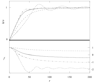
FIG. 1.: The field configurations (above) and the metric function f(r) (below) of the global monopole solutions for $v=0.15$ (dashed line), $0.25$ (solid line), $0.30$ (dot-dashed line) and $0.34$ (dotted line). The solutions except for $v=0.15$ have a cosmological horizon. The solutions for $v>\sqrt{2/8\pi}\approx 0.28$ show oscillating behavior.

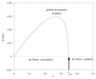
FIG. 2.: The diagram of $v$ versus $h^{\prime}$ at $r=0$. The solid and the dashed line represent the monopole and the de Sitter solutions, respectively. The stability here means against the spherical perturbations. This figure says that the monopole solutions and de Sitter solution with $v<v_{max}$ are stable against the spherical perturbations. $v_{max}$ is the bifurcation point which connects the stable de Sitter, the global monopole, and the unstable de Sitter solutions.

III Instability of de Sitter solutions

Now, we investigate time dependent perturbations of the de Sitter solutions which are non-spherical in the internal space. We perturb one component of the $O(3)$ scalar field

$$\Phi^{1}(t,r)\equiv\Phi^{2}(t,r)\equiv 0,\;\;\;\Phi^{3}(t,r)=e^{i\sigma t}\zeta(r).$$ (12)

Note that the metric functions are not affected by this perturbation since the back reaction is second order, and we can consider the de Sitter spacetime as a background. If the perturbation equation allows a solution with imaginary $\sigma$, the mode function evolves exponentially with time. That indicates instability of the de Sitter solution.

The perturbation equation is written as,

$$\frac{1}{r^{2}}\left[r^{2}f\zeta^{\prime}\right]\!^{\prime}+\lambda v^{2}\zeta=-f^{-1}\sigma^{2}\zeta.$$ (13)

Adopting the tortoise coordinate $r_{*}$,

$$\frac{dr}{dr_{*}}=f,$$ (14)

and a new variable $\bar{\zeta}=r\zeta$, we can rewrite it in the Schrödinger equation,

$$-\frac{d^{2}\bar{\zeta}}{dr_{*}^{2}}+U(r)\bar{\zeta}=\sigma^{2}\bar{\zeta}.$$ (15)

$U(r)$ is the potential function of the linear equation

$$U(r)=-f\lambda v^{2}\left(1+\frac{4}{3}\pi v^{2}\right).$$ (16)

The potential function never becomes positive inside the cosmological horizon. This is the exactly the same form as the Eqs. (37)-(39) in Ref. [19] in the de Sitter case. In that paper it was shown that these equations always have at lease one negative eigenmode for any value of $\lambda$ and $v$. Hence, it is concluded that all the de Sitter solutions which we consider here are unstable.

IV Polar perturbation of the scalar field

Since the de Sitter solutions have polar instabilities, the self-gravitating global monopoles may inherit them. Hence we study the polar perturbation of the global monopoles in general relativity carefully in this section and the following section.

The polar deformation of the $O(3)$ scalar field was proposed by Goldhaber[10]. He introduced a new coordinate $y:=\ln\tan(\theta/2)$ to discuss the invariance of the energy under the deformation. Achúcarro and Urrestilla improved his notation[13],

$$\Phi^{1} = H(t,r,\theta)\sin\bar{\theta}(t,r,\theta)\cos\phi,$$ (17)

$$\Phi^{2} = H(t,r,\theta)\sin\bar{\theta}(t,r,\theta)\sin\phi,$$ (18)

$$\Phi^{3} = H(t,r,\theta)\cos\bar{\theta}(t,r,\theta),$$ (19)

and

$$\tan(\bar{\theta}/2)=e^{y+\xi(t,r,\theta)}.$$ (20)

$\bar{\theta}$ is the polar component of $\Phi^{a}$ and $H(t,r,\theta)=h(r)+\delta h(t,r,\theta)$. When $\xi=0$, i.e., $\bar{\theta}=\theta$ and $\delta h=\delta h(t,r)$ the global monopole is spherically symmetric, while it become a ‘string’ when $\xi\rightarrow\infty$. The energy of the static global monopole is expressed with new coordinate $y$,

$$E = \int drdyd\phi(\rho_{1}+\rho_{2}),$$ (21)

where

$$\rho_{1} = \frac{H^{2}}{2}\left[\sin^{2}\bar{\theta}+\left(\frac{\partial\bar{\theta}}{\partial y}\right)^{2}+\frac{r^{2}}{\cosh^{2}y}\left(\frac{\partial\bar{\theta}}{\partial r}\right)^{2}\right],$$ (22)

$$\rho_{2} = \frac{1}{2}\left(\frac{\partial H}{\partial y}\right)^{2}+\frac{r^{2}}{2\cosh^{2}y}\left[\left(\frac{\partial H}{\partial r}\right)^{2}+\frac{1}{2}(H^{2}-v^{2})^{2}\right].$$ (23)

In the far region from the monopole core, the terms $\partial H/\partial r$ and $\partial H/\partial y$ can be disregarded. Goldhaber pointed out that the first two terms in $\rho_{1}$ are in the same form as the energy of a sine-Gordon soliton, which implies that the energy is invariant under translation of coordinate $y$ (or $\xi$). Thus, he concluded that the global monopoles have instability if there is a deviation in which $H=v$ and $\partial\bar{\theta}/\partial r=0$ are held. Rhie and Bennett proved, however, that such a collapse does not occur, if the monopole core is free to move[11].

We assume $\xi$ and $\delta h$ are small. Therefore we take

$$\bar{\theta} = \theta+\xi\sin\theta.$$ (25)

Now we have two perturbative functions $\xi$ and $\delta h$ for the $O(3)$ scalar field. The simplest polar perturbation assumes that $\delta h=0$ and $\xi$ is independent of $\theta$. However, this is inconsistent. In a non-relativistic case, such perturbation must vanish through a perturbation equation. If $\xi$ has $\theta$ dependence, we will get

$$\partial_{\theta}\xi+2\xi\cot\theta=0.$$ (26)

The solution of this equation is $\xi\propto(\sin\theta)^{-2}$, which is unphysical because $\xi$ violates the perturbative approximation around the axis.

The same feature appears in the case that only $\delta h$ is considered. Consequently, we can conclude that perturbation only with either $\xi$ or $\delta h$ does not occur when the self-gravity is set to zero. We will find that this is true also in the self-gravitating case.

Now, we assume $\xi$ is independent of $\theta$. Since we will examine the $l=1$ Legendre type perturbation below, we take $\delta h=\eta(r)\cos\theta e^{i\sigma t}$. The perturbed scalar field is

$$\Phi^{1} = (h+\eta\cos\theta e^{i\sigma t})\sin\theta\cos\phi+h\xi e^{i\sigma t}\sin\theta\cos\theta\cos\phi,$$ (27)

$$\Phi^{2} = (h+\eta\cos\theta e^{i\sigma t})\sin\theta\sin\phi+h\xi e^{i\sigma t}\sin\theta\cos\theta\sin\phi,$$ (28)

$$\Phi^{3} = (h+\eta\cos\theta e^{i\sigma t})\cos\theta-h\xi e^{i\sigma t}\sin^{2}\theta.$$ (29)

Let us consider the combination

$$p(r)=h\xi+\eta,\;\;\;q(r)=h\xi.$$ (31)

in Eq. (LABEL:eqn:ptb). Putting $p(r)\equiv 0$, we recover the polar perturbation of the de Sitter solution

$$\Phi^{1}\equiv\Phi^{2}\equiv 0,\;\;\;\Phi^{3}=-q(r)e^{i\sigma t}.$$ (32)

which is discussed in Sec. III.

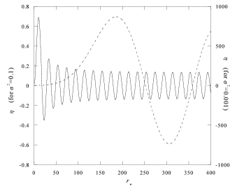
FIG. 3.: The eigenmodes of $\eta$ and $h\xi/v$ for $\sigma=0.1$ (solid line) and $0.001$ (dashed line) when $v=0.25$. We can see the oscillating behavior. These are continuous modes.

V polar perturbation of the global monopole

Achúcarro and Urrestilla studied stability of the global monopoles against polar perturbation with all orders[13] and found that the global monopoles are stable. Here we extend their analysis to the self-gravitating cases.

For the global monopole solutions, the matter field is non-zero. So the first order perturbations of the matter field couple to 0-th order to create the metric perturbations, which can be described as

$$ds^{2} = -fe^{-2\delta}e^{\delta\nu}dt^{2}+\frac{1}{f}e^{\delta\mu_{2}}dr^{2}+r^{2}e^{\delta\mu_{3}}d\theta^{2}+r^{2}\sin^{2}\theta e^{\delta\psi}d\phi^{2}.$$ (33)

The valuables in the metric can be separated [20],

$$\delta\nu = \sum N_{l}(t,r)P_{l}(\cos\theta),$$ (34)

$$\delta\mu_{2} = \sum L_{l}(t,r)P_{l}(\cos\theta),$$ (35)

$$\delta\mu_{3} = \sum[T_{l}(t,r)P_{l}(\cos\theta)+S_{l}(t,r)P_{l,\theta,\theta}(\cos\theta)],$$ (36)

$$\delta\psi = \sum[T_{l}(t,r)P_{l}(\cos\theta)+S_{l}(t,r)P_{l,\theta}(\cos\theta)\cot\theta],$$ (37)

where $P_{l}$ is a Legendre polynomial. Now we consider the simplest case $l=1$ and drop the suffix $l$. For the higher order Legendre polynomials, the eigenvalue $\sigma^{2}$ is expected to be larger than that for $l=1$. Thus, the perturbed metric can be written in the form,

$$ds^{2} = -\left[f+B(r)e^{i\sigma t}\cos\theta\right]e^{-2\delta}dt^{2}+\frac{1}{f}\left[1+L(r)e^{i\sigma t}\cos\theta\right]dr^{2}+r^{2}\left[1+T(r)e^{i\sigma t}\cos\theta\right](d\theta^{2}+\sin^{2}\theta d\phi^{2}).$$ (38)

Here, we introduced a new variable $B(r):=N(r)f(r)$ for convenience, re-defined $T:=T-S$ and assumed harmonic time dependence.

The energy momentum tensor is,

$${T_{t}}^{t} = \stackrel{{\scriptstyle\mbox{$(0)$}}}{{T}}\!^{t}_{t}+\Biggl{[}-fh^{\prime}\eta^{\prime}+\frac{fh^{{}^{\prime}2}}{2}L-\frac{2h}{r^{2}}(h\xi+\eta)+\frac{h^{2}}{r^{2}}T-\lambda h(h^{2}-v^{2})\eta\Biggr{]}\cos\theta e^{i\sigma t},$$ (39)

$${T_{r}}^{r} = \stackrel{{\scriptstyle\mbox{$(0)$}}}{{T}}\!^{r}_{r}+\Biggl{[}fh^{\prime}\eta^{\prime}-\frac{fh^{{}^{\prime}2}}{2}L-\frac{2h}{r^{2}}(h\xi+\eta)+\frac{h^{2}}{r^{2}}T-\lambda h(h^{2}-v^{2})\eta\Biggr{]}\cos\theta e^{i\sigma t},$$ (40)

$${{T}_{t}}^{r} = i\sigma fh^{\prime}\eta\cos\theta e^{i\sigma t},$$ (42)

$${{T}_{t}}^{\theta} = i\sigma\frac{h^{2}}{r^{2}}\xi\sin\theta e^{i\sigma t},$$ (43)

where $\stackrel{{\scriptstyle\mbox{$(0)$}}}{{T}}\!_{t}^{t}$ and $\stackrel{{\scriptstyle\mbox{$(0)$}}}{{T}}\!_{r}^{r}$ are non-perturbed components. We displayed only the first order perturbation. Thus, we can get the perturbation equations

$$L+T=16\pi h^{2}\xi,$$ (44)

$$f(-rT^{\prime}+L-rT\delta^{\prime}-T)+\frac{1}{2}f^{\prime}rT=8\pi rfh^{\prime}\eta,$$ (45)

$$fr^{2}T^{\prime\prime}-(frL)^{\prime}+\frac{1}{2}f^{\prime}T^{\prime}r^{2}+3frT^{\prime}-L=4\pi\left[-2fr^{2}h^{\prime}\eta^{\prime}+fr^{2}h^{\prime 2}L+2h^{2}T-4h(h\xi+\eta)\right.\left.-2r^{2}\lambda h(h^{2}-v^{2})\eta\right],$$ (46)

$$fr^{2}T^{\prime\prime}-frL^{\prime}-L+2frT^{\prime}-2fr\delta^{\prime}L+r^{2}f\delta^{\prime}T^{\prime}-\frac{r^{2}\sigma^{2}e^{2\delta}}{f}T-B^{\prime}r+\frac{B}{f}+\frac{Brf^{\prime}}{f}=8\pi r^{2}fh^{\prime}\left(h^{\prime}L+2\eta^{\prime}\right),$$ (47)

from the Einstein equation, and

$$\frac{\sigma^{2}he^{2\delta}}{f}\xi+f(h\xi)^{\prime\prime}+\left(\frac{2}{r}f+f^{\prime}-\delta^{\prime}f\right)(h\xi)^{\prime}-\frac{2\eta+2h\xi}{r^{2}}+\frac{hL}{2r^{2}}-\frac{1}{2}\frac{hB}{fr^{2}}=\lambda h(h^{2}-v^{2})\xi,$$ (48)

$$\frac{\sigma^{2}e^{2\delta}}{f}\eta+f\eta^{\prime\prime}+\left(\frac{2}{r}f+f^{\prime}-\delta^{\prime}f\right)\eta^{\prime}+fh^{\prime}T^{\prime}-\left[\frac{2h}{r^{2}}+\lambda h(h^{2}-v^{2})\right]L-\frac{4h\xi+4\eta-2hT}{r^{2}}$$ (49)

$$\;\;\;\;-\frac{fh^{\prime}L^{\prime}}{2}+\frac{1}{2}h^{\prime}B^{\prime}-\frac{h^{\prime}f^{\prime}B}{2f}=\lambda(3h^{2}-v^{2})\eta,$$ (50)

from the equation of the scalar field.

The boundary conditions at $r=0$ are obtained by imposing regularity. By Taylor expansion around $r=0$, we find

$$\xi = \xi_{1}r+O\left(r^{3}\right),$$ (51)

$$\eta = \frac{h_{1}}{4}(8\xi_{1}-B_{1})r^{2}+O\left(r^{4}\right),$$ (52)

$$B = B_{1}r-\frac{1}{6}\left(m_{3}+\frac{24}{5}\pi h_{1}^{2}\right)B_{1}r^{3}+O\left(r^{5}\right),$$ (53)

$$T = \frac{2}{5}\pi h_{1}^{2}B_{1}r^{3}+O\left(r^{5}\right),$$ (54)

$$L = \left(16\pi\xi_{1}-\frac{2}{5}\pi B_{1}\right)h_{1}^{2}r^{3}+O\left(r^{5}\right),$$ (55)

where $F_{n}$ represents the n-th order derivative coefficient of $F$ at $r=0$. We assumed all values at $r=0$ are $0$, for the elimination of trivial translations mode in which $\eta=-h^{\prime}\cos\theta$ and $h\xi=h/r$ [13]. This assumption is not, however, an artificial fixing of the core, but only coordinate transformation. The values of $h_{1}$ and $m_{3}$ are given by the static solutions in Sec. II. $\xi_{1}$ and $B_{1}$ cannot be determined by this regularity condition. Among these, $\xi_{1}$ is arbitrary because of the freedom of the constant multiplication in the linear theory. Hence there are two parameters $B_{1}$ and $\sigma^{2}$ in this system, which should be adjusted to obtain the regular normalizable eigenmodes. If there is no solution, we cannot find an appropriate set of $B_{1}$ and $\sigma^{2}$.

By these boundary conditions we solve Eqs. (44)-(50) numerically. Fig. 3 is the typical solution of the supermassive case. We can find the oscillating behavior for the positive eigenvalue $\sigma^{2}$. These are the continuum modes.

If we neglect self-gravity, the perturbation equations become quite simple. In this case it is easy to observe that the potential function is nonzero constant asymptotically to infinity. Hence there is a minimum value of the eigenvalue $\sigma_{min}^{2}=2\lambda v^{2}>0$ for the continuous modes. When self-gravity is taken into account, the situation does not change seriously for the ordinary global monopole solution. The existence of the minimum eigenvalue is seen in Fig. 4. Although $\sigma_{min}\!^{2}$ decreases continuously for large $B_{1}$, it converges to a positive constant which is smaller than that of the non-self-gravitating case.

For the supermassive global monopole, however, the form of the potential function is qualitatively different due to the existence of the cosmological horizon. It vanishes at the horizon without bottom up, and hence the continuous modes exist for the infinitesimally small eigenvalue as seen in Fig. 5.

Figure 6 shows the “zero modes” ($\sigma^{2}=0$), which diverge and are non-normalizable, for several values of $v$. We cannot find a real zero-mode solution for any value of $B_{1}$ while there exists a solution for non-zero positive $\sigma^{2}$. When a negative eigenmode exists in this kind of linear perturbation analysis, the perturbed functions have at least one zero point for $\sigma^{2}=0$ in general. In our case, “zero modes” are positive everywhere. This indicates that the self-gravitating supermassive global monopoles are stable against the polar perturbations as well as the spherical perturbations. As $v$ approaches its maximum value $v_{max}$, the “zero modes” become small. It is expected that it has zero when $v=v_{max}$. This behavior is consistent with the instability of the de Sitter solution discussed in Sec. III.

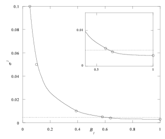
FIG. 4.: The diagram of the shooting parameter $B_{1}$ versus $\sigma^{2}$ when $v=0.15$. The background global monopole solution does not have a cosmological horizon. We can see $\sigma^{2}$ converges to positive constant for large $B_{1}$. The horizontal line is minimum eigenvalue $\sigma_{min}:=2\lambda v^{2}$ in the non-self-gravitating case. The asymptotic value of $\sigma^{2}$ for the self-gravitating case is smaller than that of the non-self-gravitating case.

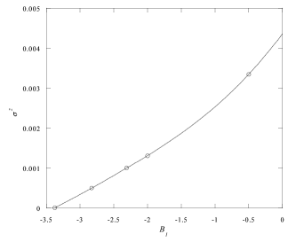
FIG. 5.: Diagram of the shooting parameter $B_{1}$ versus $\sigma^{2}$ when $v=0.25$, which corresponds to the case of the supermassive global monopoles. We can see that $\sigma^{2}$ is continuously decreasing to $0$, but there is no zero mode as seen in Fig. 6.

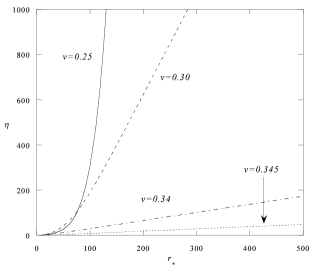
FIG. 6.: “Zero modes” of the supermassive global monopoles. We can see that the “zero modes” are positive and have no zero point. This indicates the stability of the supermassive monopoles. At $v=\sqrt{3/8\pi}\approx 0.345$, the supermassive global monopole coincides with the de Sitter solution, which is unstable. This figure shows that the “zero modes” would have zero point as $v\to v_{max}$.

VI Discussion

We investigated the polar stability of the self-gravitating supermassive global monopoles and de Sitter solutions in the Einstein-$O(3)$ scalar system by the linear perturbation method [13]. Although the de Sitter solutions always have at least one unstable mode for any value of the VEV of the scalar field, the supermassive global monopole solutions do not. This implies that the supermassive global monopoles are stable against polar perturbations. We also find that the minimum eigenvalue is infinitesimal for the supermassive global monopoles while it becomes non-zero finite for the ordinary self-gravitating global monopoles and non-gravitating counterparts. This is due to the different boundary conditions at the cosmological horizon.

Our analysis can be extended to the black hole solution inside of the monopole, i.e., the black hole solution with $O(3)$ scalar hair. Such solution was discovered a decade ago[21, 18] and its supermassive counterpart was recently discovered by Maison and Liebling[15]. It was reported that these solutions are stable against spherical perturbations. This result is notable because this scalar hair can be a physical hair. Hence we should check whether or not this hair is stable also against polar perturbations. It should be noted however, that even if this hair is absolutely stable, it does not mean the violation of the the black hole no-hair conjecture, because such conjecture is implicitly assumed in the asymptotic flatness. Some attempts to extend the conjecture to asymptotically non-flat spacetime were discussed in Ref. [22, 23].

REFERENCES

- [1] M. Barriola and A. Vilenkin, Phys. Rev. Lett. 63, 341 (1989).
- [2] A.Vilenkin, Phys. Rev. Lett. 72, 3137 (1994).
- [3] A.D.Linde, Phys. Lett. B 327, 208 (1994).
- [4] N. Sakai, H. Shinkai, T. Tachizawa and K. Maeda, Phys. Rev. D53, 655 (1996).
- [5] S. L. Liebling, Phys. Rev. D61, 024030 (1999).
- [6] P. Laguna and D. Garfinkle, Phys. Rev. D40 1011 (1989).
- [7] D. Maison, gr-qc/9912100.
- [8] U. Nucamendi and D. Sudarsky, Class. Quantum Grav. 17, 4051 (2000).
- [9] G. H. Derrick, J. Math. Phys. 5, 1252 (1964).
- [10] A. S. Goldhaber, Phys. Rev. Lett. 63, 2158 (1989).
- [11] S. H. Rhie and D. P. Bennett, Phys. Rev. Lett. 67, 1173 (1991).
- [12] L. Periviolaropoulos, Nucl. Phys. B375, 665 (1992).
- [13] A. Achúcarro and J. Urrestilla, Phys. Rev. Lett. 85, 3091 (2000).
- [14] D. P. Bennett and S. H. Rhie, Phys. Rev. Lett. 65, 1709 (1990).
- [15] D. Maison, and S. L. Liebling, Phys. Rev. Lett. 83, 5218 (1999).
- [16] P. Breitenlohner and D. Z. Freedmann, Phys. Lett. B 115, 197 (1982).
- [17] K. Maeda, T. Tachizawa, T. Torii and T. Maki, Phys. Rev. Lett. 72, 450 (1994); T. Torii, K. Maeda and T. Tachizawa, Phys. Rev. D51, 1510 (1995).
- [18] T. Tachizawa, K. Maeda and T. Torii, Phys. Rev. D51, 4054 (1995).
- [19] T. Torii, K. Maeda and M. Narita, Phys. Rev. D59, 104002 (1999).
-
[20]
J.L.Friedman, Proc. Roy. Soc. A335, 163 (1973);
Chandrasekhar, The Mathematical Theory of Black Holes (OXFORD, 1983). - [21] K. Lee, V. P. Nair and E. J. Weinberg, Phys. Rev. D45, 2751 (1992); M. E. Ortiz, Phys. Rev. D45, R2586 (1992); P. Breitenlohner, F. Forgács, and D. Maison, Nucl. Phys. B383, 357 (1992);
- [22] T. Torii, K. Maeda and M. Narita, Phys. Rev. D59, 064027 (1999).
- [23] T. Torii, K. Maeda and M. Narita, Phys. Rev. D64, 044007 (2001).