Energy Norms and the Stability of the Einstein Evolution Equations

Abstract

The Einstein evolution equations may be written in a variety of equivalent analytical forms, but numerical solutions of these different formulations display a wide range of growth rates for constraint violations. For symmetric hyperbolic formulations of the equations, an exact expression for the growth rate is derived using an energy norm. This expression agrees with the growth rate determined by numerical solution of the equations. An approximate method for estimating the growth rate is also derived. This estimate can be evaluated algebraically from the initial data, and is shown to exhibit qualitatively the same dependence as the numerically-determined rate on the parameters that specify the formulation of the equations. This simple rate estimate therefore provides a useful tool for finding the most well-behaved forms of the evolution equations.

I Introduction

It is well known that the Einstein equations may be written in a variety of forms Arnowitt et al. (1962); York (1979); Shibata and Nakamura (1995); Baumgarte and Shapiro (1999); Fischer and Marsden (1979); Bona and Massó (1992); Frittelli and Reula (1994); Bona et al. (1995); Choquet-Bruhat and York (1995); Abrahams et al. (1995); van Putten and Eardley (1996); Frittelli and Reula (1996); Friedrich (1996); Estabrook et al. (1997); Iriondo et al. (1997); Anderson et al. (1997); Bonilla (1998); Yoneda and Shinkai (1999); Anderson and York (1999); Frittelli and Reula (1999); Alcubierre et al. (1999); Hern (1999); Friedrich and Rendall (2000); Yoneda and Shinkai (2000); Shinkai and Yoneda (2000); Kidder et al. (2001); Yoneda and Shinkai (2001); Shinkai and Yoneda (2002); Alvi (2002); Sarbach and Tiglio (2002); Yoneda and Shinkai (2002); Laguna and Shoemaker (2002). In recent years a growing body of work has documented the fact that these different formulations, while equivalent analytically, have significantly different stability properties when used for unconstrained  numerical evolutions Scheel et al. (1998); Baumgarte and Shapiro (1999); Shinkai and Yoneda (2000); Kidder et al. (2001); Laguna and Shoemaker (2002); Alcubierre et al. (2000a); Calabrese et al. (2002). The most important of these differences is the behavior of non-physical solutions of the evolution equations, which often grow exponentially and eventually dominate the desired physical solutions. These non-physical solutions could be solutions of the evolution equations that violate the constraints (“constraint-violating instabilities”) or solutions that satisfy the constraints but represent some ill-behaved coordinate transformation (“gauge instabilities”). In many cases it is the rapid exponential growth of these non-physical solutions, rather than numerical issues, that appear to be the key factor that limits our ability to run numerical simulations of black holes for long times Scheel et al. (1998); Alcubierre et al. (2000b); Kidder et al. (2001); Knapp et al. (2002). For lack of a better term, we refer to these non-physical solutions as “instabilities” (because they are unstable, i.e., exponentially-growing, solutions of the evolution equations), but keep in mind that they are neither numerical instabilities nor do they represent physics.

In this paper we explore the use of the energy norm (which can be introduced for any symmetric hyperbolic form of the evolution equations) to study these instabilities. We derive an exact expression for the growth rate in terms of the energy norm, and verify that the rate determined in this way agrees with the growth rate of the constraint violations determined numerically. We also derive an approximate expression for this growth rate that can be evaluated algebraically from the initial data for the evolution equations. We explore the accuracy of this approximation by comparing it with numerically-determined growth rates for solutions of a family of symmetric hyperbolic evolution equations.

In order to compare the analytical expressions for the growth rates derived here with the results of numerical computations, it is necessary to select some particular family of evolution equations with which to make the comparisons. Here we focus our attention on the 12-parameter family of first-order evolution equations introduced by Kidder, Scheel, and Teukolsky (KST) Kidder et al. (2001). This family of equations has been shown to be strongly hyperbolic when certain inequalities are satisfied by the 12 parameters; however, our expressions for the instability growth rates apply only to symmetric hyperbolic systems of equations. Therefore we must extend the analysis of the KST equations by explicitly constructing the symmetrizer (or metric on the space of fields) that makes the equations symmetric hyperbolic. We show that such a symmetrizer (in fact a four-parameter family of such symmetrizers) can be constructed for an open subset of the KST equations having only physical characteristic speeds.

We compare numerical evolutions of the symmetric hyperbolic subset of the KST equations with our analytical expressions (both exact and approximate) for the growth rates of the instabilities. We make these comparisons using two sets of initial data for the evolution equations: flat space in Rindler coordinates Wald (1984), and the Schwarzschild geometry in Painlevé-Gullstrand coordinates Painlevé (1921); Gullstrand (1922); Martel and Poisson (2001). We find that our exact analytic expression for the growth rate of the instability agrees with the actual growth rate of the constraints in (both fully nonlinear and linearized) numerical simulations. This agreement provides further evidence that the constraint-violating instabilities are real features of the evolution equations and not an artifact of using a poor numerical algorithm. In addition, the approximate analytical expressions for the growth rates derived here are shown to have good qualitative agreement with the numerically-determined rates. This approximation therefore provides a useful tool for finding more well-behaved formulations of the equations. Furthermore, the growth rate of the instability is shown here to depend in a non-trivial way on the exact “background” solution as well as on the particular formulation of the equations. Hence, unfortunately, it seems likely that it will never be possible to find a unique “most stable” form of the equations for the evolution of all initial data.

II Energy Norms and Rate Estimates

We limit our study here to formulations of the Einstein evolution equations that can be expressed as first-order systems

$$\partial_{t}u^{\alpha}+A^{k\alpha}{}_{\beta}\partial_{k}u^{\beta}=F^{\alpha}.$$ (1)

Here $u^{\alpha}$ is the collection of dynamical fields, $A^{k\alpha}{}_{\beta}$ and $F^{\alpha}$ are (generally complicated) functions of $u^{\alpha}$, and $\partial_{t}$ and $\partial_{k}$ are the partial derivatives with respect to the time $t$ and the spatial coordinates $x^{k}$ respectively. (We use Greek indices to label the dynamical fields and Latin indices to label spatial components of tensors.) Systems of equations of the form (1) are called weakly hyperbolic Kreiss and Lorenz (1989) if $n_{k}A^{k\alpha}{}_{\beta}$ has all real eigenvalues for all spatial one-forms $n_{k}$, and strongly hyperbolic if in addition $n_{k}A^{k\alpha}{}_{\beta}$ has a complete set of eigenvectors for all $n_{k}$. There exists a large literature devoted to a variety of representations of the Einstein evolution equations that satisfy these conditions Fischer and Marsden (1979); Bona and Massó (1992); Frittelli and Reula (1994); Bona et al. (1995); Choquet-Bruhat and York (1995); Abrahams et al. (1995); van Putten and Eardley (1996); Frittelli and Reula (1996); Friedrich (1996); Estabrook et al. (1997); Iriondo et al. (1997); Anderson et al. (1997); Bonilla (1998); Yoneda and Shinkai (1999); Anderson and York (1999); Frittelli and Reula (1999); Alcubierre et al. (1999); Hern (1999); Friedrich and Rendall (2000); Yoneda and Shinkai (2000); Shinkai and Yoneda (2000); Kidder et al. (2001); Yoneda and Shinkai (2001); Shinkai and Yoneda (2002); Alvi (2002); Sarbach and Tiglio (2002). In particular, the 12-parameter KST system of equations that we use for our numerical comparisons is of this form.

In order to construct an energy norm, first-order systems such as Eq. (1) must have an additional structure: a “symmetrizer” $S_{\alpha\beta}$. First-order systems of evolution equations are called symmetric hyperbolic Kreiss and Lorenz (1989) (or symmetrizable hyperbolic) if there exists a symmetrizer which serves as a metric on the space of fields. Such a symmetrizer must be symmetric and positive definite (i.e. $S_{\alpha\beta}u^{\alpha}u^{\beta}>0,\,\,\,\forall\,\,u^{\alpha}\neq 0$); in addition, it must symmetrize the matrices $A^{k\alpha}{}_{\beta}$: $S_{\alpha\mu}A^{k\mu}{}_{\beta}\equiv A^{k}_{\alpha\beta}=A^{k}_{\beta\alpha},\,\,\,\forall\,\,{\scriptstyle k}$. In this paper we limit our discussion to symmetric hyperbolic formulations. Note that symmetric hyperbolic systems are automatically strongly hyperbolic, because symmetric matrices $n_{k}A^{k}_{\alpha\beta}$ always have real eigenvalues with a complete set of eigenvectors. But the converse is not true: strongly hyperbolic systems need not be symmetric hyperbolic (except in one spatial dimension). In Sec. III we construct symmetrizers for (an open subset of) the KST equations.

Let us turn now to the question of the stability of the evolution equations. To do this we consider solutions to the equations that are close (as defined by the metric $S_{\alpha\beta}$) to an exact “background” solution $u^{\alpha}_{e}$ . Note that $u^{\alpha}_{e}$ may be time-dependent. We define $\delta u^{\alpha}=u^{\alpha}-u^{\alpha}_{e}$ to be the deviation of the solution $u^{\alpha}$ from this given background solution. The evolution of $\delta u^{\alpha}$ is determined by the linearized evolution equations:

$$\partial_{t}\delta u^{\alpha}+A^{k\alpha}{}_{\beta}\partial_{k}\delta u^{\beta}=F^{\alpha}{}_{\beta}\delta u^{\beta}.$$ (2)

Here $A^{k\alpha}{}_{\beta}$ and $F^{\alpha}{}_{\beta}$ may depend on $u^{\alpha}_{e}$ but not on $\delta u^{\alpha}$. We illustrate in Fig. 1 below that the constraint-violating instabilities occur in the solutions to these linearized evolution equations as well as in the solutions to the full non-linear equations.

II.1 Energy Evolution

For any symmetric hyperbolic system of evolution equations, we may define a natural “energy density” and “energy-flux” Courant and Hilbert (1962); Gustafsson et al. (1995) associated with $\delta u^{\alpha}$:

$$\delta E = S_{\alpha\beta}\delta u^{\alpha}\delta u^{\beta},$$ (3)

$$\delta E^{k} = A^{k}_{\alpha\beta}\delta u^{\alpha}\delta u^{\beta}.$$ (4)

It follows immediately from the linearized evolution equations Eq. (2) that this energy density evolves as follows,

$$\partial_{t}\,\delta E+\nabla_{k}\,\delta E^{k}=C_{\alpha\beta}\delta u^{\alpha}\delta u^{\beta},$$ (5)

where $\nabla_{k}$ is the spatial covariant derivative associated with the (background) three-metric $g_{ij}$, $C_{\alpha\beta}$ is given by

$$C_{\alpha\beta} = 2S_{\mu(\alpha}F^{\mu}{}_{\beta)}+\partial_{t}S_{\alpha\beta}$$ (6)

$$+(\sqrt{g})^{-1}\partial_{k}\bigl{(}\sqrt{g}A^{k}_{\alpha\beta}\bigr{)},$$

and $g=\det g_{ij}$ is the determinant of the (background) spatial metric. Note that $C_{\alpha\beta}$, which serves as the source (or sink) for the energy in (5), depends on $u^{\alpha}_{e}$ but not on $\delta u^{\alpha}$.

II.2 Exact Expression for the Growth Rate

Next we explore the possibility of using this energy to measure and to estimate the growth rate of instabilities. Define the growth rate $1/\tau$ of the energy norm to be

$$\frac{1}{\tau}=\frac{\partial_{\,t}||\delta E||}{2||\delta E||},$$ (7)

where the energy norm $||\delta E||$ is defined by

$$||\delta E||=\int\delta E\sqrt{g}\,d^{\,3}x.$$ (8)

Integrating Eq. (5) over a $t$=constant surface, we obtain the following general expression for the growth rate of the energy norm:

$$\frac{1}{\tau}=\frac{1}{2||\delta E||}\int\left(C_{\alpha\beta}\delta u^{\alpha}\delta u^{\beta}-\nabla_{n}\delta E^{n}\right)\sqrt{g}\,d^{\,3}x.$$ (9)

We note that Eq. (9) is an identity for any solution of the equations. The rate $1/\tau$ becomes independent of time when $\delta u^{\alpha}$ grows exponentially: $\delta u^{\alpha}\propto e^{t/\tau}$.

Figure 1 illustrates the equivalence between the energy norm measure and the standard measures of the growth rate of the constraint-violating instability. Plotted are results from 3D nonlinear numerical evolutions of perturbed Schwarzschild initial data using a particular formulation of the Einstein evolution equations . The solid curves show the evolution of the energy norm $||\delta E||$ while the dotted curves show the evolution of the norm of the constraint violations,

$$||{\cal C}||\equiv\int\bigl{(}{\cal C}^{2}+{\cal C}_{i}{\cal C}^{i}\bigr{)}\sqrt{g}\,d^{\,3}x,$$ (10)

where ${\cal C}$ represents the Hamiltonian and ${\cal C}_{i}$ the momentum constraints . The larger points plotted in Fig. 1 show the energy norm computed for a numerical solution of the linearized evolution equations, indicating that the constraint-violating instabilities occur even in the linearized theory.

Figure 1: Energy norm $||\delta E||$ and constraints $||{\cal C}||$ (per unit volume) for evolutions of perturbed Schwarzschild initial data using three spectral resolutions. Solid curves are $||\delta E||$ from the full non-linear evolution code, and points are from the linearized code. Dotted curves are $||{\cal C}||$ from the non-linear code.

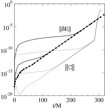
Figure 1 clearly illustrates that the constraint violations $||{\cal C}||$ grow at the same rate as the energy norm $||\delta E||$ (until the very end of the simulation when non-linear effects become significant). This equality between the growth rates is exact for any constraint-violating solution having the form $\delta u^{\alpha}(t,\vec{x})=e^{t/\tau}\delta u^{\alpha}(0,\vec{x})$. Our numerical solution approaches this form asymptotically. The numerically-determined slopes of these curves, $1/\tau({\delta E_{L}})=0.0489$ (from the linear evolution code), $1/\tau({\delta E_{NL}})=0.0489$ (from the non-linear code) and $1/\tau({\cal C})=0.0490$ (also from the non-linear code), are also in good agreement with the growth rate determined from the integral expression in Eq. (9): $1/\tau({\scriptscriptstyle\int})=0.0489$. This agreement shows that the numerical solutions satisfy the identity in Eq. (9). This provides further strong evidence that the constraint-violating instabilities seen here are real solutions to the evolution equations, rather than arising from purely numerical problems associated with the discrete representation of the solution or the time-evolution algorithm.

The computational domain, boundary conditions, initial data, and other details of the numerical evolutions shown in Fig. 1 are the same as described later in Section IV.2. To choose gauge conditions we set the shift and the densitized lapse equal to their analytic values for all time. Each nonlinear evolution in Fig. 1 is shown for three different spectral resolutions, 18x8x15, 24x8x15, and 32x8x15 (where the notation $N_{r}$x$N_{\theta}$x$N_{\phi}$ represents the number of spectral collocation points in the $r$, $\theta$, and $\phi$ directions), demonstrating the asymptotic convergence of these results. The results for the same three resolutions using the linear evolution code are indistinguishable from each other in Fig. 1, so only one resolution is plotted. These linearized results are also essentially indistinguishable (until very late times) from the highest resolution non-linear results.

II.3 Approximate Expression for the Growth Rates

Although Eq. (9) is an identity, it does not provide a particularly useful way to determine $1/\tau$. Its use requires the full knowledge of the spatial structure of the unstable solution $\delta u^{\alpha}$, and this can be determined only by solving the equations. Our goal is to obtain a reasonable estimate of $1/\tau$ without having to solve the evolution equations.

We first note that if $\delta E^{k}\,n_{k}\geq 0$ at the boundaries (where $n_{k}$ is the outward-directed normal one-form at the boundary), one can integrate (9) by parts and obtain

$$\frac{1}{\tau}\leq\frac{1}{2||\delta E||}\int C_{\alpha\beta}\delta u^{\alpha}\delta u^{\beta}\,\sqrt{g}d^{\,3}x.$$ (11)

Therefore if $\lambda_{\rm max}$ is the largest eigenvalue $\lambda$ of the equation $0=(C_{\alpha\beta}-\lambda S_{\alpha\beta})\delta u^{\beta}$, then

$$\frac{1}{\tau}\leq\frac{\lambda_{\rm max}}{2},$$ (12)

or equivalently,

$$||\delta E||\leq C||\delta E_{(t=0)}||e^{\lambda_{\rm max}t}$$ (13)

for some constant $C$. This argument is often used Gustafsson et al. (1995) to show that symmetric hyperbolic systems have well-posed initial value problems, i.e., that symmetric hyperbolic systems have growth rates that are bounded by exponentials. Because our numerical simulations use boundary conditions that satisfy $\delta E^{k}n_{k}\geq 0$ (incoming characteristic fields are zero), we could use (12) to estimate the growth rate. Unfortunately, we find that the upper bound provided by (12) is typically far greater than the actual growth rate, and therefore an estimate based on this bound is not very useful.

Therefore we take a different approach. Without any prior knowledge of the structure of the actual unstable solution, the simplest choice is to assume that the spatial gradients are given approximately by $\partial_{n}\delta u^{\alpha}\approx k_{n}\delta u^{\alpha}$, where $k_{n}$ is a “wavevector” that characterizes the direction and magnitude of the gradient of $\delta u^{\alpha}$. (Since the actual solutions that are responsible for the instabilities in the cases we have studied do seem to have a characteristic lengthscale, typically the mass of the black hole or some other physically distinguished scale, this approximation should not be too bad.) In this case the expression in Eq. (9) for $1/\tau$ simplifies to

$$\frac{1}{\tau}=\frac{1}{2||\delta E||}\int\bar{C}_{\alpha\beta}\delta u^{\alpha}\delta u^{\beta}\sqrt{g}\,d^{\,3}x,$$ (14)

where $\bar{C}_{\alpha\beta}$ is given by

$$\bar{C}_{\alpha\beta}=2S_{\mu(\alpha}F^{\mu}{}_{\beta)}+\partial_{t}S_{\alpha\beta}-2k_{n}A^{n}_{\alpha\beta}.$$ (15)

Next we limit the $\delta u^{\alpha}$ to the subspace of field vectors that satisfy the boundary conditions. We do this formally for these $\delta u^{\alpha}$ by introducing the projection operator $P^{\alpha}{}_{\beta}$. This projection annihilates vectors that violate the boundary conditions, and leaves those vectors that satisfy all the boundary conditions unchanged . Using this projection we re-write Eq. (14) as

$$\frac{1}{\tau}=\frac{1}{2||\delta\tilde{E}||}\int\bar{C}_{\alpha\beta}P^{\alpha}{}_{\mu}P^{\beta}{}_{\nu}\delta u^{\mu}\delta u^{\nu}\sqrt{g}\,d^{\,3}x,$$ (16)

where $\delta\tilde{E}=S_{\alpha\beta}P^{\alpha}{}_{\mu}P^{\beta}{}_{\nu}\delta u^{\mu}\delta u^{\nu}$. We expect that the fastest growing solution to the evolution equation will be the one driven most strongly by these “source” terms on the right side of Eq. (16). Thus we approximate (roughly) this most unstable solution as the eigenvector $\delta e^{\alpha}$ of $\bar{C}_{\alpha\beta}P^{\alpha}{}_{\mu}P^{\beta}{}_{\nu}$ having the largest eigenvalue:

$${\bar{\lambda}}_{\max}S_{\alpha\beta}P^{\alpha}{}_{\mu}P^{\beta}{}_{\nu}\delta e^{\nu}=\bar{C}_{\alpha\beta}P^{\alpha}{}_{\mu}P^{\beta}{}_{\nu}\delta e^{\nu}.$$ (17)

The integrals in Eq. (16) are easily evaluated for this eigenvector $\delta e^{\alpha}$, giving the following approximate expression for the growth rate,

$$\frac{1}{\tau}\approx\frac{1}{2\int\delta\tilde{E}\sqrt{g}\,d^{\,3}x}\int{\bar{\lambda}}_{\max}\delta\tilde{E}\sqrt{g}\,d^{\,3}x=\frac{{\bar{\lambda}}_{\max}}{2}.$$ (18)

In this approximation then the growth rate of this most unstable solution is half the maximum eigenvalue of $\bar{C}_{\alpha\beta}P^{\alpha}{}_{\mu}P^{\beta}{}_{\nu}$. We test the accuracy of this approximation in Sec. IV by comparing its predictions with the results of numerical solutions to the evolution equations.

III Einstein Evolution Equations

In this Section we introduce the particular formulations of the Einstein evolution equations that we study numerically to make comparisons with the growth rate estimates derived in Sec. II. The rather general 12-parameter family of formulations introduced by Kidder, Scheel, and Teukolsky (KST) Kidder et al. (2001) is ideal for these purposes. In this Section we review these formulations and derive expressions for the symmetrizer $S_{\alpha\beta}$ and energy density $\delta E$ (when they exist) that are needed for our growth rate estimates. This Section contains a very brief review of the derivation and basic properties of the KST equations using the notation of this paper, followed by a rather more detailed and technical derivation of the needed symmetrizer and energy norms. Readers more interested in our numerical tests of the growth rate estimates might prefer to skip ahead to that material in Sec. IV.

III.1 Summary of the KST Equations

The KST formulation of the Einstein evolution equations begins with the standard ADM Arnowitt et al. (1962) equations (discussed in detail in York (1979)) written as a first-order system for the “fundamental” dynamical variables: $u^{\alpha}_{0}=\{g_{ij},K_{ij},D_{kij}\}$, where $g_{ij}$ is the spatial metric, $K_{ij}$ is the extrinsic curvature, and $D_{kij}\equiv{\scriptstyle\frac{1}{2}}\partial_{k}g_{ij}$. We express these standard ADM equations in the (somewhat abstract) form:

$$\partial_{\,t}g{}_{ij} = N^{k}\partial_{k}g_{ij}+2g_{k(i}\partial_{j)}N^{k}-2NK_{ij},$$ (19)

$$\partial_{\,t}K_{ij} = \cdots,$$ (20)

$$\partial_{\,t}D_{kij} = \cdots,$$ (21)

where $N$ and $N^{k}$ are the lapse and shift respectively. The $\,\,\cdots\,\,$ on the right sides of Eqs. (20) and (21) stand for the standard terms that appear in the first-order form of the ADM equations, which are given explicitly (up to a slight change in notation ) in Eqs. (2.14) and (2.24) of KST Kidder et al. (2001). The 12-parameter extension of these equations proposed by KST splits naturally into two parts: the first part has 5 dynamical parameters (represented by Greek letters $\gamma$, $\zeta$, $\eta$, $\chi$, and $\sigma$) that influence the dynamics (e.g. including the characteristic speeds) of the system in a fundamental way, and the second part has 7 kinematical parameters (represented by Latin letters $\hat{z}$, $\hat{k}$, $\hat{a}$, $\hat{b}$, $\hat{c}$, $\hat{d}$, and $\hat{e}$) that merely re-define the dynamical fields.

The 5-parameter family of dynamical modifications of these equations is obtained a) by adding a 4-parameter family of multiples of the constraints to the fundamental ADM equations, and b) by assuming that a certain densitized lapse function (which depends on one additional parameter) rather than the lapse itself, is a fixed function on spacetime. The first modification is obtained by adding multiples of the constraints to the right sides of Eqs. (20) and (21):

$$\partial_{\,t}K_{ij} = \cdots\,\,+\gamma Ng_{ij}{\cal C}+\zeta Ng^{ab}{\cal C}_{a(ij)b},$$ (22)

$$\partial_{\,t}D_{kij} = \cdots\,\,+{\scriptstyle\frac{1}{2}}\eta Ng_{k(i}{\cal C}_{j)}+{\scriptstyle\frac{1}{2}}\chi Ng_{ij}{\cal C}_{k},$$ (23)

where $\gamma$, $\zeta$, $\eta$, and $\chi$ are constants, and the constraints (for the vacuum case) are defined by

$${\cal C} = {\scriptstyle\frac{1}{2}}[{}^{(3)}R-K_{ij}K^{ij}+K^{2}],$$ (24)

$${\cal C}_{i} = \nabla_{j}K^{j}{}_{i}-\nabla_{i}K,$$ (25)

$${\cal C}_{kij} = \partial_{k}g_{ij}-D_{kij},$$ (26)

$${\cal C}_{klij} = \partial_{k}D_{lij}-\partial_{l}D_{kij}.$$ (27)

The second modification comes by assuming that the densitized lapse $Q$, defined by

$$Q=\log(Ng^{-\sigma}),$$ (28)

(rather than the lapse itself) is a fixed function on spacetime, where $g=\det(g_{ij})$ and $\sigma$ is a constant. With these modifications the extended ADM equations become a 5-parameter family of evolution equations for the fundamental fields $u^{\alpha}_{0}$. These equations can be written as

$$\partial_{\,t}u^{\alpha}_{0}+A_{0}^{k\alpha}{}_{\beta}\partial_{\,k}u^{\beta}_{0}=F^{\alpha}_{0}.$$ (29)

The quantities $A^{k}_{0}{}^{\alpha}{}_{\beta}$ and $F^{\alpha}_{0}$ are functions of the fields $u^{\alpha}_{0}$ and the parameters $\gamma$, $\zeta$, $\eta$, $\chi$, and $\sigma$. We give explicit expressions for the $A^{k}_{0}{}^{\alpha}{}_{\beta}$ in Sec. III.2 and the Appendix.

The 12-parameter KST family of representations of the Einstein evolution equations is completed by adding a 7-parameter family of kinematical transformations of the dynamical fields to the fundamental representations given in Eq. (29). These transformations replace $K_{ij}$ and $D_{kij}$ by $P_{ij}$ and $M_{kij}$ according to the expressions:

$$P_{ij}=K_{ij}+\hat{z}\,g_{ij}g^{ab}K_{ab},$$ (30)

$$M_{kij}=\bigl{[}\hat{k}\,\delta^{a}_{k}\delta^{b}_{i}\delta^{c}_{j}+\hat{e}\,\delta^{a}_{(i}\delta^{b}_{j)}\delta^{c}_{k}+\hat{a}\,g_{ij}g^{bc}\delta^{a}_{k}+\hat{b}\,g_{ij}g^{ab}\delta^{c}_{k}$$

$$\quad\qquad\quad+\hat{c}\,g_{k(i}\delta^{a}_{j)}g^{bc}+\hat{d}\,g_{k(i}\delta^{c}_{j)}g^{ab}\bigr{]}D_{abc}.$$ (31)

While these kinematical transformations may seem like “trivial” re-parameterizations of the theory, numerical results (see e.g. Sec. IV.2 below) have shown that these transformations can have a significant effect on the stability of the equations. The general transformation defined in Eqs. (30) and (31) is a linear transformation from the basic dynamical fields $u^{\alpha}_{0}$ to the new set of dynamical fields $u^{\alpha}=\{g_{ij},P_{ij},M_{kij}\}$:

$$u^{\alpha}=T^{\alpha}{}_{\beta}u^{\beta}_{0},$$ (32)

where the transformation $T^{\alpha}{}_{\beta}$ depends on the kinematical parameters and the metric $g_{ij}$. The special case with $\hat{k}=1$ and $\hat{z}=\hat{a}=\hat{b}=\hat{c}=\hat{d}=\hat{e}=0$ corresponds to the identity transformation $u^{\alpha}=u^{\alpha}_{0}$. The explicit representations of the inverse transformation $(T^{-1})^{\,}{}^{\alpha}{}_{\beta}$ are given in the Appendix.

The evolution equations for the new transformed dynamical fields $u^{\alpha}$ are obtained by multiplying Eq. (29) by $T^{\alpha}{}_{\beta}$. The result (after some straightforward manipulation) has the same general form as Eq. (29),

$$\partial_{\,t}u^{\alpha}+A^{k\alpha}{}_{\beta}\partial_{\,k}u^{\beta}=F^{\alpha},$$ (33)

with $A^{k}{}^{\alpha}{}_{\beta}$ and $F^{\alpha}$ given by:

$$A^{k\alpha}{}_{\beta} = T^{\alpha}{}_{\mu}A^{k\mu}_{0}{}_{\nu}(T^{-1})^{\,\nu}{}_{\beta},$$ (34)

$$F^{\alpha} = T^{\alpha}{}_{\beta}F^{\beta}_{0}+V^{\alpha ij}\partial_{t}g_{ij}+2A^{k}{}^{\alpha}{}_{\beta}V^{\beta ij}D_{kij},\qquad\quad$$ (35)

where $V^{\alpha ij}$ is defined by

$$V^{\alpha ij}=\frac{\partial T^{\alpha}{}_{\mu}}{\partial g_{ij}}(T^{-1}){}^{\mu}{}_{\nu}u^{\nu}.$$ (36)

All of the terms on the right side of Eq. (35), except the term containing $\partial_{t}g_{ij}$, depend on the $u^{\alpha}$ (or $u^{\alpha}_{0}=T^{-1}{}^{\alpha}{}_{\beta}u^{\beta}$) and not its derivatives. In the remaining term, the quantity $\partial_{t}g_{ij}$ is to be replaced by the right-hand side of Eq. (19); this introduces the spatial derivatives $\partial_{k}g_{ij}$, which are to be replaced by $2D_{kij}$. Thus in the end $F^{\alpha}$ in Eq. (35) is simply a function of $u^{\alpha}$ as required.

The simple transformation (34) that relates the matrix $A^{k\mu}_{0}{}_{\nu}$ of the fundamental representation of the equations with $A^{k\mu}{}_{\nu}$ ensures that the characteristic speeds of the theory are independent of the kinematical parameters:

$$0=\det\left(-v\delta^{\alpha}{}_{\beta}+n_{k}A^{k\alpha}{}_{\beta}\right)=\det\left(-v\delta^{\alpha}{}_{\beta}+n_{k}A^{k\alpha}_{0}{}_{\beta}\right).$$ (37)

These characteristic speeds (relative to the hypersurface orthogonal observers) are also independent of direction $n_{k}$ in general relativity. Thus the hyperbolicity of these formulations can depend only on the dynamical parameters $\gamma$, $\zeta$, $\eta$, $\chi$, and $\sigma$. One can show that these characteristic speeds (relative to the hypersurface orthogonal observers) are $\{0,\pm 1,\pm v_{1},\pm v_{2},\pm v_{3}\}$, where

$$v_{1}^{2} = 2\sigma,$$ (38)

$$v_{2}^{2} = {\scriptstyle\frac{1}{8}}\left(\eta-4\eta\sigma-2\chi-12\sigma\chi-3\eta\zeta\right),$$ (39)

$$v_{3}^{2} = {\scriptstyle\frac{1}{2}}\left(2+4\gamma-\eta-2\gamma\eta+2\chi+4\gamma\chi-\eta\zeta\right).\qquad$$ (40)

In much of the analysis that follows, we will restrict attention to the subset of these KST equations where the characteristic speeds have only the physical values $\{0,\pm 1\}$. This requires $v_{1}^{2}=v_{2}^{2}=v_{3}^{2}=1$ if the theory is also to be strongly hyperbolic (see KST Kidder et al. (2001)). Thus our primary focus will be the 9-parameter family of equations in which the parameters $\sigma$, $\eta$, and $\chi$ are fixed by the conditions,

$$\sigma = {\scriptstyle\frac{1}{2}},$$ (41)

$$\eta = {-8\over 5+7\zeta+10\gamma+6\gamma\zeta},$$ (42)

$$\chi = -{4+4\zeta+10\gamma+6\gamma\zeta\over 5+7\zeta+10\gamma+6\gamma\zeta},$$ (43)

that are needed to ensure $v_{1}=v_{2}=v_{3}=1$. The parameters $\gamma$ and $\zeta$ are arbitrary so long as $5+7\zeta+10\gamma+6\gamma\zeta\neq 0$. Thus the curve $\gamma=-(7\zeta+5)/(6\zeta+10)$ is forbidden, but $\gamma$ and $\zeta$ are otherwise unconstrained .

III.2 Symmetric Hyperbolicity of KST

A first order system such as Eq. (33) is called symmetric hyperbolic if there exists a positive definite symmetrizer $S{}_{\alpha\beta}$ such that $A{}^{n}_{\alpha\beta}\equiv S{}_{\alpha\gamma}A{}^{n\gamma}{}_{\beta}$ is symmetric in the indices $\alpha$ and $\beta$, $A{}^{n}_{\alpha\beta}=A{}^{n}_{\beta\alpha}$, for all field configurations. We assume here that $S{}_{\alpha\beta}$ depends only on the spatial metric $g{}_{ij}$ . It is convenient to represent the symmetrizer as a quadratic form

$$dS^{2}=S{}_{\alpha\beta}du{}^{\alpha}du{}^{\beta},$$ (44)

where $du{}^{\alpha}=\{dg{}_{ij},dP_{ij},dM_{kij}\}$ denotes the standard basis of co-vectors on the space of dynamical fields. The most general symmetric quadratic form on the space of dynamical fields (which depends only on the metric $g{}_{ij}$) is given by

$$dS^{2}=A_{1}\,dG^{2}+B{}_{1}\,dP^{2}+2D_{1}\,dGdP$$

$$\quad+A_{2}\,g{}^{ik}g{}^{jl}d\tilde{g}{}_{ij}d\tilde{g}{}_{kl}+B{}_{2}\,g{}^{ik}g{}^{jl}d\tilde{P}{}_{ij}d\tilde{P}{}_{kl}$$

$$\quad+2D_{2}\,g{}^{ik}g{}^{jl}d\tilde{g}_{ij}d\tilde{P}_{kl}+C{}_{1}g{}^{kl}g{}^{ia}g{}^{jb}d\tilde{M}{}_{(kij)}d\tilde{M}_{(lab)}$$

$$\quad+C{}_{2}g{}^{kl}g{}^{ia}g{}^{jb}\bigl{[}d\tilde{M}{}_{kij}-d\tilde{M}{}_{(kij)}\bigr{]}\bigl{[}d\tilde{M}_{lab}-d\tilde{M}_{(lab)}\bigr{]}$$

$$\quad+C{}_{3}\,g{}^{ij}dM{}^{1}_{i}dM{}^{1}_{j}+C{}_{4}\,g{}^{ij}dM{}^{2}_{i}dM{}^{2}_{j}$$

$$\quad+2C{}_{5}\,g{}^{ij}dM{}^{1}_{i}dM{}^{2}_{j}.$$ (45)

Here $dG$ and $dP$ are the traces of $dg_{ij}$ and $dP{}_{ij}$ respectively, and $d\tilde{g}{}_{ij}$ and $d\tilde{P}{}_{ij}$ are their trace-free parts. The two traces of $dM{}_{kij}$ are defined by

$$dM{}^{1}_{i} \equiv dM{}_{ijk}g{}^{jk}$$ (46)

$$dM{}^{2}_{i} \equiv dM{}_{kij}g{}^{jk},$$ (47)

and its trace-free part, $d\tilde{M}{}_{kij}$, is

$$d\tilde{M}{}_{kij}\equiv dM{}_{kij} + {\scriptstyle\frac{1}{5}}\bigl{[}dM{}^{1}_{(i}g{}_{j)k}-2\,dM{}^{1}_{k}g{}_{ij}$$ (48)

$$\quad+dM{}^{2}_{k}g{}_{ij}-3\,dM{}^{2}_{(i}g{}_{j)k}\bigr{]}.\qquad$$

This quadratic form, Eq. (45), is positive definite iff $\{A_{1},A_{2},B_{1},B_{2},C_{1},C_{2},C_{3},C_{4}\}$ are all positive and $C_{5}^{2}<C_{3}C_{4}$, $D_{1}^{2}<A_{1}B_{1}$, and $D_{2}^{2}<A_{2}B_{2}$. (The signs of $C_{5}$, $D_{1}$ and $D_{2}$ are irrelevant.)

The question now is whether the constants $A{}_{A}$, $B{}_{A}$, $C{}_{A}$ and $D_{A}$ can be chosen to make the $A{}^{n}_{\alpha\beta}$ symmetric in $\alpha$ and $\beta$. In order to answer this we need explicit expressions for the matrices $A^{n\alpha}{}_{\beta}$. Quite generally these matrices are determined for these equations by a set of 12 constants $\mu_{A}$ and $\nu_{A}$, which in turn are determined by the 12 parameters of the KST formulations. (We give the explicit expressions for $\mu_{A}$ and $\nu_{A}$ in terms of the KST parameters in the Appendix.) The equations that define the $A^{n\,\alpha}{}_{\beta}$ in terms of these constants are:

$$\partial{}_{t}g{}_{ij} \simeq N^{n}\partial_{n}g_{ij},$$ (49)

$$\partial{}_{t}P{}_{ij} \simeq N^{n}\partial_{n}K_{ij}-N\Bigl{[}\mu{}_{1}g{}^{nb}\delta{}^{c}{}_{i}\delta{}^{d}{}_{j}+\mu{}_{2}g{}^{nd}\delta{}^{b}{}_{(i}\delta{}^{c}{}_{j)}$$ (50)

$$+\mu{}_{3}g{}^{bc}\delta{}^{n}{}_{(i}\delta{}^{d}{}_{j)}+\mu{}_{4}g{}^{cd}\delta{}^{n}{}_{(i}\delta{}^{b}{}_{j)}$$

$$+\mu{}_{5}g{}^{nd}g{}^{bc}g{}_{ij}+\mu{}_{6}g{}^{nb}g{}^{cd}g{}_{ij}\Bigr{]}\partial{}_{k}M{}_{bcd},$$

$$\partial{}_{t}M{}_{kij} \simeq N^{n}\partial_{n}M_{kij}-N\Bigl{[}\nu{}_{1}\delta{}^{n}{}_{k}\delta{}^{b}{}_{i}\delta{}^{c}{}_{j}+\nu{}_{2}\delta{}^{n}{}_{(i}\delta{}^{b}{}_{j)}\delta{}^{c}{}_{k}$$ (51)

$$+\nu{}_{3}g{}^{nb}g{}_{k(i}\delta{}^{c}{}_{j)}+\nu{}_{4}g{}^{nb}g{}_{ij}\delta{}^{c}{}_{k}$$

$$+\nu{}_{5}g{}^{bc}g{}_{k(i}\delta{}^{n}{}_{j)}+\nu{}_{6}g{}^{bc}g{}_{ij}\delta{}^{n}{}_{k}\Bigr{]}\partial{}_{n}P{}_{bc},$$

where $\simeq$ means that only the principal parts of the equations have been represented explicitly ($\partial_{t}u^{\alpha}+A^{n\,\alpha}{}_{\beta}\partial_{k}u^{\beta}\simeq 0$).

We now evaluate $A^{n}_{\alpha\beta}=S_{\alpha\mu}A^{n\,\mu}{}_{\beta}$ and $A^{n}_{\beta\alpha}=S_{\beta\mu}A^{n\,\mu}{}_{\alpha}$ using the expressions in Eqs. (45) through (51). After lengthy algebraic manipulations, we find that $A^{n}_{\alpha\beta}$ is symmetric iff $D_{1}=D_{2}=0$ and the following constraints are satisfied by the constants $B{}_{A}$ and $C{}_{A}$:

$$0 = B_{2}(\mu_{1}+\mu_{2})-C_{1}(\nu_{1}+\nu_{2}),$$ (52)

$$0 = B_{2}(2\mu_{1}-\mu_{2})-C_{2}(2\nu_{1}-\nu_{2}),\qquad$$ (53)

$$0 = B_{1}(3\mu_{1}+3\mu_{4}+9\mu_{6})$$ (54)

$$-C_{3}(3\nu_{1}+\nu_{2}+\nu_{3}+3\nu_{4}+3\nu_{5}+9\nu_{6})$$

$$-C_{5}(\nu_{1}+2\nu_{2}+2\nu_{3}+\nu_{4}+6\nu_{5}+3\nu_{6}),$$

$$0 = B_{1}(3\mu_{2}+3\mu_{3}+9\mu_{5})$$ (55)

$$-C_{5}(3\nu_{1}+\nu_{2}+\nu_{3}+3\nu_{4}+3\nu_{5}+9\nu_{6})$$

$$-C_{4}(\nu_{1}+2\nu_{2}+2\nu_{3}+\nu_{4}+6\nu_{5}+3\nu_{6}),$$

$$0 = B_{2}(-2\mu_{1}+3\mu_{2}+10\mu_{4})-C_{3}(10\nu_{2}+10\nu_{3}+30\nu_{4})$$ (56)

$$-C_{5}(10\nu_{1}+5\nu_{2}+20\nu_{3}+10\nu_{4}),$$

$$0 = B_{2}(~{}~{}6\mu_{1}+~{}~{}\mu_{2}+10\mu_{3})-C_{5}(10\nu_{2}+10\nu_{3}+30\nu_{4})$$ (57)

$$-C_{4}(10\nu_{1}+5\nu_{2}+20\nu_{3}+10\nu_{4}).$$

This is a system of six linear equations for the seven parameters $B{}_{A}$ and $C{}_{A}$. Thus we expect there to exist solution(s) to these equations for almost all choices of the $\mu_{A}$ and $\nu_{A}$. However, there is no guarantee that such solutions will satisfy the positivity requirements needed to ensure that $S_{\alpha\beta}$ is positive definite.

We divide into two parts the question of determining when solutions to Eqs. (52) through (57) exist that satisfy the appropriate positivity conditions: first the question of when a positive definite symmetrizer, $S^{0}_{\alpha\beta}$, exists for the subset of the KST equations whose dynamical fields are the fundamental fields $u^{\alpha}_{0}$, and second the question of when this fundamental symmetrizer can be extended to a symmetrizer for the full 12-parameter set of KST equations. We consider the second question first. Assume that for a given set of dynamical parameters there exists a positive definite $S^{0}_{\alpha\beta}$ such that $S^{0}_{\alpha\gamma}A^{n\gamma}_{0}{}_{\beta}=S^{0}_{\beta\gamma}A^{n\gamma}_{0}{}_{\alpha}$. Now define $S_{\alpha\beta}$:

$$S_{\alpha\beta}=T^{-1\,\mu}{}_{\alpha}S^{0}_{\mu\nu}T^{-1\,\nu}{}_{\beta}.$$ (58)

One can verify, using Eq. (34), that this $S_{\alpha\beta}$ symmetrizes $A^{n\alpha}{}_{\beta}$. Further it follows, using Eq. (32), that this $S_{\alpha\beta}$ is positive definite,

$$S_{\alpha\beta}u^{\alpha}u^{\beta}=S^{0}_{\alpha\beta}u^{\alpha}_{0}u^{\beta}_{0}>0,$$ (59)

since $S^{0}_{\alpha\beta}$ is assumed to be positive definite. In the Appendix we give explicit expressions for the constants $B_{A}$ and $C_{A}$ that define $S_{\alpha\beta}$ in terms of the constants $B^{0}_{A}$ and $C^{0}_{A}$ that define $S^{0}_{\alpha\beta}$ and the parameters that define the transformation $T^{-1}{}^{\alpha}{}_{\beta}$.

Now we return to the first, and more difficult, question: when does there exist a positive definite symmetrizer $S^{0}_{\alpha\beta}$ for the subset of the KST equations whose dynamical fields are the fundamental fields $u^{\alpha}_{0}$? At the present time we have not solved this problem completely. Rather, we restrict our attention to an interesting (perhaps the most interesting) subset of these KST equations in which the characteristic speeds $v_{1}$, $v_{2}$ and $v_{3}$ are all the speed of light: $v_{1}=v_{2}=v_{3}=1$. The restrictions that these conditions place on the dynamical parameters are given in Eqs. (41) through (43). Each of these systems is strongly hyperbolic.

One can now evaluate the $\mu_{A}$ and $\nu_{A}$ appropriate for this subset of KST equations using Eqs. (120) through (127) along with Eqs. (41) through (43). Substituting these into Eqs. (52) through (57) gives the symmetrization conditions for these equations. These conditions are degenerate in this case, reducing to only five independent equations. Solving these five symmetrization equations for the $C_{A}^{0}$ in terms of the $B_{A}^{0}$ gives

$$C_{1}^{0} = -\zeta B_{2}^{0},$$ (60)

$$C_{2}^{0} = {\scriptstyle\frac{1}{2}}(3+\zeta)B_{2}^{0},$$ (61)

$$C_{3}^{0} = 9(1+\gamma)^{2}B_{1}^{0}+{3(\zeta-5)^{2}\over 10(5+3\zeta)}B_{2}^{0},$$ (62)

$$C_{4}^{0} = (2+3\gamma)^{2}B_{1}^{0}+{(9\zeta-5)^{2}\over 30(5+3\zeta)}B_{2}^{0},$$ (63)

$$C_{5}^{0} = -3(1+\gamma)(2+3\gamma)B_{1}^{0}$$ (64)

$$\qquad-{(\zeta-5)(9\zeta-5)\over 10(5+3\zeta)}B_{2}^{0}.$$

These equations guarantee that $\{C_{1}^{0},C_{2}^{0},C_{3}^{0},C_{4}^{0}\}$ are positive for any positive $B_{1}^{0}$ and $B_{2}^{0}$ if and only if

$$0>\zeta>-{\scriptstyle\frac{5}{3}}.$$ (65)

The only remaining condition needed to establish symmetric hyperbolicity is to ensure that $C_{3}^{0}C_{4}^{0}-(C_{5}^{0})^{2}>0$. Using Eqs. (62) through (64) it follows that

$$C_{3}^{0}C_{4}^{0}-(C_{5}^{0})^{2}={3(5+7\zeta+10\gamma+6\gamma\zeta)^{2}\over 10(5+3\zeta)}B_{1}^{0}B_{2}^{0}.$$ (66)

Thus the right side is positive whenever $B_{1}^{0}$ and $B_{2}^{0}$ are positive iff $\zeta>-{\scriptstyle\frac{5}{3}}$ and $5+7\zeta+10\gamma+6\gamma\zeta\neq 0$. The first of these conditions along with Eq. (60) demonstrates that Eq. (65) is the necessary and sufficient constraint on the parameters $\{\zeta,\gamma\}$ to ensure symmetric hyperbolicity. The second of these conditions was also required to ensure that the parameters $\eta$ and $\chi$ in Eqs. (42) and (43) are finite, so it does not represent a new restriction.

Thus a large open set of this two-parameter family of the fundamental KST representations of the Einstein evolution equations is symmetric hyperbolic. And perhaps even more surprising, the complimentary subset of these strongly hyperbolic equations (i.e. when $\zeta>0$ or $\zeta<-{\scriptstyle\frac{5}{3}}$) is not symmetric hyperbolic . Further, the extension of this two-parameter family via Eq. (58) produces a nine-parameter family of strongly hyperbolic representations the Einstein equations. A large open subset of this nine-parameter family is symmetric hyperbolic (i.e. those that are extensions of the symmetric hyperbolic fundamental representations), while its compliment is not symmetric hyperbolic.

The construction used here to build a symmetrizer $S_{\alpha\beta}$ for the KST equations has succeeded unexpectedly well. We found not just a single symmetrizer, but in fact a four-parameter family of such symmetrizers. Using the expressions for the $C_{A}$ from Eqs. (60) through (64), we see that the symmetrizer $S^{0}_{\alpha\beta}$ is a sum of terms that depend linearly on each of the four parameters $\{A_{1},A_{2},B^{0}_{1},B^{0}_{2}\}$. Thus we may write this symmetrizer in the form:

$$S^{0}_{\alpha\beta}=A_{1}S^{10}_{\alpha\beta}+A_{2}S^{20}_{\alpha\beta}+B^{0}_{1}S^{30}_{\alpha\beta}+B^{0}_{2}S^{40}_{\alpha\beta},$$ (67)

where the “sub-symmetrizers” $S^{A0}_{\alpha\beta}$ represent a set of positive definite (under the conditions needed for symmetric hyperbolicity established above) metrics on mutually orthogonal subspaces in the space of fields $u^{\alpha}$. The expressions for these sub-symmetrizers are

$$S^{10}_{\alpha\beta}du^{\alpha}du^{\beta}=dG^{2},$$ (68)

$$S^{20}_{\alpha\beta}du^{\alpha}du^{\beta}=g^{ij}g^{kl}d\tilde{g}_{ij}d\tilde{g}_{kl},$$ (69)

$$S^{30}_{\alpha\beta}du^{\alpha}du^{\beta}=dP^{2}+g^{ij}\bigl{[}3(1+\gamma)dM^{1}_{i}-(2+3\gamma)dM^{2}_{i}\bigr{]}$$ (70)

$$\qquad\qquad\qquad\times\bigl{[}3(1+\gamma)dM^{1}_{j}-(2+3\gamma)dM^{2}_{j}\bigr{]},\quad$$

$$S^{40}_{\alpha\beta}du^{\alpha}du^{\beta}=g^{ik}g^{jl}d\tilde{P}_{ij}d\tilde{P}_{kl}-\zeta g^{kl}g^{ia}g^{jb}d\tilde{M}_{(kij)}\tilde{d}M_{(lab)}$$ (71)

$$\quad+\bigl{[}30(5+3\zeta)\bigr{]}^{-1}g^{ij}\bigl{[}3(\zeta-5)dM^{1}_{i}-(9\zeta-5)dM^{2}_{i}\bigr{]}$$

$$\qquad\qquad\qquad\times\bigl{[}3(\zeta-5)dM^{1}_{j}-(9\zeta-5)dM^{2}_{j}\bigr{]}$$

$$\quad+{\scriptstyle\frac{1}{3}}(3+\zeta)g^{kl}g^{ia}g^{jb}\bigl{[}d\tilde{M}_{kij}-d\tilde{M}_{(kij)}\bigr{]}$$

$$\qquad\qquad\qquad\times\bigl{[}d\tilde{M}_{lab}-d\tilde{M}_{(lab)}\bigr{]}.$$

The dimensions of the corresponding sub-spaces are $\{1,5,4,20\}$. Just as the fundamental symmetrizer $S^{0}_{\alpha\beta}$ is related to the more general symmetrizer $S_{\alpha\beta}$ by the transformation given in Eq. (58), so the fundamental sub-symmetrizers are related to the general sub-symmetrizers by,

$$S^{A}_{\alpha\beta}=T^{-1\,\mu}{}_{\alpha}S^{A0}_{\mu\nu}T^{-1\,\nu}{}_{\beta}.$$ (72)

We note that this transformation leaves the first two sub-symmetrizers unchanged: $S^{1}_{\alpha\beta}=S^{10}_{\alpha\beta}$ and $S^{2}_{\alpha\beta}=S^{20}_{\alpha\beta}$.

One interesting subset of the nine-parameter family of KST equations studied here is the two-parameter “generalized Einstein-Christoffel” system studied extensively by KST Kidder et al. (2001). In the language used here this two-parameter family is defined by

$$\zeta = -\hat{k}=-1,$$ (73)

$$\hat{a} = \gamma+3\hat{z}+3\hat{z}\gamma,$$ (74)

$$\hat{b} = -\gamma-2\hat{z}-3\gamma\hat{z},$$ (75)

$$\hat{c} = -\hat{d}=2,$$ (76)

$$\hat{e} = 0.$$ (77)

Substituting these parameter values into Eqs. (60) through (64) and (153) through (159), we find the constants that determine the symmetrizer to be

$$B^{0}_{1} = (1+3\hat{z})^{2}B_{1},$$ (78)

$$B^{0}_{2} = C_{1}=C_{2}=B_{2},$$ (79)

$$C_{3} = B_{1}+{\scriptstyle\frac{1}{15}}B_{2},$$ (80)

$$C_{4} = {\scriptstyle\frac{3}{5}}B_{2},$$ (81)

$$C_{5} = -{\scriptstyle\frac{1}{5}}B_{2},$$ (82)

where $B_{1}$ and $B_{2}$ are arbitrary positive constants. For this case the sub-symmetrizers $S^{3}_{\alpha\beta}$ and $S^{4}_{\alpha\beta}$ have the simple forms:

$$S^{3}_{\alpha\beta}du^{\alpha}du^{\beta}=dP^{2}+g^{ij}dM^{1}_{i}dM^{1}_{j},\hfill$$ (83)

$$S^{4}_{\alpha\beta}du^{\alpha}du^{\beta}=g^{kl}g^{ia}g^{jb}dM_{kij}dM_{lab}-{\scriptstyle\frac{1}{3}}g^{ij}dM^{1}_{i}dM^{1}_{j}\hfill$$

$$\qquad\qquad\qquad+g^{ik}g^{jl}dP_{ij}dP_{kl}-{\scriptstyle\frac{1}{3}}dP^{2}.$$ (84)

We also point out that the symmetrizer becomes particularly simple in this generalized Einstein-Christoffel case by taking $A_{1}=B_{1}={\scriptstyle\frac{1}{3}}$ and $A_{2}=B_{2}=1$:

$$dS^{2}=S_{\alpha\beta}du^{\alpha}du^{\beta} = g^{ik}g^{jl}dg_{ij}dg_{kl}+g^{ik}g^{jl}dP_{ij}dP_{kl}$$ (85)

$$+g^{kl}g^{ia}g^{jb}dM_{kij}dM_{lab}.$$

This represents a kind of “Euclidean” metric on the space of fields, in which the symmetrizer is just the sum of squares of the components of the dynamical fields.

III.3 The KST Energy Norms

The symmetrizers for the KST equations may be written as arbitrary positive linear combinations of the sub-symmetrizers as in Eq. (67). Since the equation for $C_{\alpha\beta}$, and hence the equation for the evolution of the energy is linear in $S_{\alpha\beta}$, it follows that there are in fact four independent energy “sub-norms” for the KST equations. Each is defined using the corresponding sub-symmetrizer:

$$\delta E_{A} = S^{A}_{\alpha\beta}\delta u^{\alpha}\delta u^{\beta},$$ (86)

$$\delta E^{n}_{A} = S^{A}_{\alpha\mu}A^{n\mu}{}_{\beta}\delta u^{\alpha}\delta u^{\beta}.$$ (87)

It follows that these energies each satisfy evolution equations analogous to Eq. (5):

$$\partial_{t}\delta E_{A}+\nabla_{n}\delta E^{n}_{A}=C^{A}_{\alpha\beta}\delta u^{\alpha}\delta u^{\beta},$$ (88)

where $C^{A}_{\alpha\beta}$ is given by

$$C^{A}_{\alpha\beta} = 2S^{A}_{\mu(\alpha}F^{\mu}{}_{\beta)}+\partial_{t}S^{A}_{\alpha\beta}$$ (89)

$$+(\sqrt{g})^{-1}\partial_{n}\bigl{(}\sqrt{g}S^{A}_{\alpha\mu}A^{n\mu}{}_{\beta}\bigr{)}.$$

Each of these energies gives the same growth rate $\tau$ from Eq. (9) for solutions that grow exponentially. At present we have not found a use for this unexpected abundance of symmetrizers and energy norms. In our numerical work below we choose (fairly arbitrarily) one member of this family to compute our growth-rate estimates.

In our earlier discussion we found it useful to analyze the symmetrizers associated with these equations in two steps: first, to consider the symmetrizers associated with the fundamental representations of the theory, and second to work out how the general symmetrizer can be obtained from the fundamental representation by performing a suitable transformation. Here we find it useful to consider the corresponding questions for the energies. First we recall that the dynamical fields $u^{\alpha}$ are related to the fundamental fields by the transformation,

$$u^{\alpha}=T^{\alpha}{}_{\beta}u^{\beta}_{0},$$ (90)

where the matrix $T^{\alpha}{}_{\beta}$ [defined in Eqs. (30) and (31)] depends on the kinematical parameters and the metric $g_{ij}$. Thus perturbations $\delta u^{\alpha}$ are related to perturbations in the fundamental fields by:

$$\delta u^{\alpha} = \left(T^{\alpha}{}_{\beta}+\partial_{\beta}T^{\alpha}{}_{\gamma}u^{\gamma}_{0}\right)\delta u^{\beta}_{0},$$ (91)

$$= T^{\alpha}{}_{\mu}\left(\delta^{\mu}{}_{\beta}+V^{\mu}{}_{\beta}\right)\delta u^{\beta}_{0},$$

where

$$V^{\alpha}{}_{\beta}=T^{-1\alpha}{}_{\gamma}\partial_{\beta}T^{\gamma}{}_{\sigma}u^{\sigma}_{0}.$$ (92)

One can now work out the transformation properties of the energy and flux using Eqs. (34) and (58):

$$\delta E = S_{\alpha\beta}\delta u^{\alpha}\delta u^{\beta},$$ (93)

$$= \delta E_{0}+S^{0}_{\mu\nu}V^{\mu\nu}_{\alpha\beta}\delta u^{\alpha}_{0}\delta u^{\beta}_{0},$$

where $V^{\mu\nu}_{\alpha\beta}$ is defined as

$$V^{\mu\nu}_{\alpha\beta}=\delta^{\mu}_{\alpha}V^{\nu}{}_{\beta}+\delta^{\mu}_{\beta}V^{\nu}{}_{\alpha}+V^{\mu}{}_{\alpha}V^{\nu}{}_{\beta}.$$ (94)

Thus the energy $\delta E$ is just the fundamental energy $\delta E_{0}=S^{0}_{\alpha\beta}\delta u^{\alpha}_{0}\delta u^{\beta}_{0}$ plus terms proportional to $V^{\mu\nu}_{\alpha\beta}$. A similar argument leads to the transformation for the energy flux:

$$\delta E^{n}=\delta E^{n}_{0}+A^{n}_{0}{}_{\mu\nu}V^{\mu\nu}_{\alpha\beta}\delta u^{\alpha}_{0}\delta u^{\beta}_{0}.$$ (95)

We note that the only dependence of the energy and flux on the kinematical parameters comes through $V^{\mu\nu}_{\alpha\beta}$ and hence $V^{\mu}{}_{\alpha}$.

Finally, we note that the expression for the transformation of the terms $C_{\alpha\beta}\delta u^{\alpha}\delta u^{\beta}$ can be obtained by a similar calculation. The result is

$$\!\!\!\!\!\!\!\!C_{\alpha\beta}\delta u^{\alpha}\delta u^{\beta}=\biggl{[}C^{0}_{\alpha\beta}+2S^{0}_{\mu\nu}V^{\mu\nu}_{\alpha\sigma}F^{\sigma}_{0\beta}+\partial_{t}\left(S^{0}_{\mu\nu}V^{\mu\nu}_{\alpha\beta}\right)$$

$$\qquad\qquad+(\sqrt{g})^{-1}\partial_{n}\left(\sqrt{g}A^{n}_{0\mu\nu}V^{\mu\nu}_{\alpha\beta}\right)+E_{\alpha\beta}\biggr{]}\delta u^{\alpha}_{0}\delta u^{\beta}_{0},$$

(96)

where the term $E_{\alpha\beta}$ is defined by

$$\!\!\!\!E_{\alpha\beta}\delta u^{\alpha}_{0}\delta u^{\beta}_{0}=-2\left(\delta^{\mu}_{\alpha}+V^{\mu}{}_{\alpha}\right)\delta u^{\alpha}_{0}S^{0}_{\mu\nu}V^{\nu}{}_{\sigma}A^{n\sigma}_{0}{}_{\beta}\partial_{n}\delta u^{\beta}_{0}$$

$$\qquad\quad\,+2\left(\delta^{\mu}_{\alpha}+V^{\mu}{}_{\alpha}\right)\delta u^{\alpha}_{0}A^{n}_{0\mu\nu}V^{\nu}{}_{\beta}\partial_{n}\delta u^{\beta}_{0}.$$ (97)

This expression is obtained by straightforward calculation using Eqs. (93) through (95). Note that the left side of Eq. (97) is a quadratic form in $\delta u^{\alpha}_{0}$ while the right side depends on the derivatives $\partial_{n}\delta u^{\alpha}_{0}$. To understand this we use the fact that $V^{\mu}{}_{\alpha}$ is non-zero only when the index $\alpha$ corresponds to one of the spatial metric components, i.e. $V^{\alpha}{}_{\beta}\delta u^{\beta}_{0}=V^{\alpha ij}\delta g_{ij}$. This follows from Eqs. (36) and (92) and the fact that $T^{\alpha}{}_{\beta}$ depends on $g_{ij}$ but none of the other dynamical fields. It follows that the term $V^{\nu}{}_{\sigma}A^{n\sigma}_{0}{}_{\beta}\partial_{n}\delta u^{\beta}_{0}$ includes only the derivatives of fields that are present in the metric evolution equation. But this evolution equation, Eq. (49), includes only the derivatives of the metric along the shift vector, and so it follows that $V^{\nu}{}_{\sigma}A^{k\sigma}_{0}{}_{\beta}=-N^{k}V^{\nu}{}_{\beta}$. Thus the expression for $E_{\alpha\beta}$ may be written in the form:

$$E_{\alpha\beta}\delta u^{\alpha}_{0}\delta u^{\beta}_{0} = 4\left(\delta^{\mu}_{\alpha}+V^{\mu}{}_{\alpha}\right)\left(A^{k}_{0\mu\nu}+N^{k}S^{0}_{\mu\nu}\right)\delta u^{\alpha}_{0}$$ (98)

$$\times V^{\nu ij}\delta D_{kij}$$

The last terms in this expression came from the term $V^{\nu}{}_{\beta}\partial_{k}\delta u^{\beta}_{0}$, which [using Eq. (36)] depends only on the spatial derivatives of the metric perturbations $\delta g_{ij}$: $V^{\nu}{}_{\beta}\partial_{k}\delta u^{\beta}_{0}=V^{\nu ij}\partial_{k}\delta g_{ij}=2V^{\nu ij}\delta D_{kij}$. Thus the right side of Eq. (98) is a quadratic form in the $\delta u^{\alpha}_{0}$ as required. Finally we note that $C_{\alpha\beta}\delta u^{\alpha}\delta u^{\beta}$, like the energy and energy-flux, depends on the kinematical parameters only through $V^{\alpha}{}_{\beta}$. The expression for the transformation of the matrix $\bar{C}_{\alpha\beta}$ that appears in our approximate expressions for the instability growth-rates, Eq. (16), follows directly from Eq. (96):

$$\!\!\!\!\!\!\!\!\bar{C}_{\alpha\beta}\delta u^{\alpha}\delta u^{\beta}=\biggl{[}\bar{C}^{0}_{\alpha\beta}+2S^{0}_{\mu\nu}V^{\mu\nu}_{\alpha\sigma}F^{\sigma}_{0\beta}+\partial_{t}\left(S^{0}_{\mu\nu}V^{\mu\nu}_{\alpha\beta}\right)$$

$$\qquad\qquad\qquad+E_{\alpha\beta}-2k_{n}A^{n}_{0\mu\nu}V^{\mu\nu}_{\alpha\beta}\biggr{]}\delta u^{\alpha}_{0}\delta u^{\beta}_{0}.$$ (99)

IV Numerical Tests

In this section we compare the approximate expressions for the instability growth rates developed in Sec. II with growth rates determined directly from numerical solutions of the Einstein evolution equations. For this study we use the 2-parameter subset of the KST equations, discussed in Sec. III.2, referred to as the generalized Einstein-Christoffel system Kidder et al. (2001). Since we do not yet understand the meaning of the different energy norms developed in Sec. III.3, we limit our consideration here to the norm computed from the symmetrizer with $A_{1}=B^{0}_{1}=1/3$ and $A_{2}=B^{0}_{2}=1$. This choice is the closest analog we have of the simple “Euclidean” metric of Eq. (85) for these systems.

We examine the accuracy of the approximate expression for the growth rate, Eq. (18), by examining the evolution of perturbations about two rather different background spacetimes: flat spacetime in Rindler coordinates Wald (1984), and the Schwarzschild geometry in Painlevé-Gullstrand coordinates Painlevé (1921); Gullstrand (1922); Martel and Poisson (2001). In each of these cases the full 3D numerical evolution of these equations has constraint-violating (and possibly gauge) instabilities, and the approximate expressions for the growth rates using our new formalism are simple enough that we can evaluate them in a straightforward manner (even analytically in some cases). Thus we are able to compare the estimates of the growth rates with the full numerical evolutions in a systematic way.

IV.1 Rindler Spacetime

Flat spacetime can be expressed in Rindler coordinates as follows,

$$ds^{2}=-x^{2}dt^{2}+dx^{2}+dy^{2}+dz^{2}.$$ (100)

In this geometry the dynamical fields have the following simple forms,

$$g_{ij} = \delta_{ij},$$ (101)

$$K_{ij} = 0,$$ (102)

$$D_{kij} = 0,$$ (103)

$$N = x,$$ (104)

$$N^{k} = 0,$$ (105)

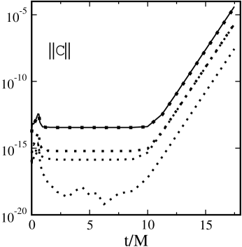
where $\delta_{ij}$ represents the Euclidean metric in Cartesian coordinates. Figure 2 illustrates that even this simple representation of flat space is subject to the constraint violating instabilities. This figure shows the evolution of the norms of each of the constraints defined in Eqs. (24) through (27). This figure also illustrates that all of the constraints grow at the same exponential rate in our simulations.

Figure 2: Solid curve shows the evolution of the sum of the integral norms of all of the constraints. Dotted curves show the individual contributions from the various constraints: ${\cal C}_{klij}{\cal C}^{klij}$, ${\cal C}{}^{2}$, ${\cal C}_{kij}{\cal C}^{kij}$, and ${\cal C}_{k}{\cal C}^{k}$ (in that order from largest to smallest).

The simplicity of the expressions (101) through (105) allows us to evaluate the various quantities needed to make our stability estimates in a reasonably straightforward way. The first consequence of this simple form is that the unperturbed fundamental fields consist only of metric fields: $u^{\alpha}_{0}=\{\delta_{ij},0,0\}$. This fact considerably simplifies many of the needed expressions. In particular, the quantity $\partial_{\alpha}T^{\mu}{}_{\nu}u^{\nu}_{0}$ vanishes identically for this geometry because $T^{\mu}{}_{\nu}$, when $\nu$ has values that correspond to the components of the metric, is just the identity transformation and hence independent of the dynamical fields. Thus the matrix $V^{\mu}{}_{\alpha}$ defined in Eq. (92) vanishes identically for the Rindler geometry. It follows that for Rindler $\delta E=\delta E_{0}$, $\delta E^{n}=\delta E^{n}_{0}$, and $C_{\alpha\beta}\delta u^{\alpha}\delta u^{\beta}=C^{0}_{\alpha\beta}\delta u^{\alpha}_{0}\delta u^{\beta}_{0}$. Thus the timescale $1/\tau$ associated with the instability in the Rindler geometry is completely independent of the kinematical parameters of the representation of the evolution equations. This independence of $1/\tau$ on the kinematical parameters has been verified numerically for the 2-parameter generalized Einstein-Christoffel subset of the linearized KST equations.

Next we evaluate the simple estimate of the growth rate of the fastest-growing mode using Eq. (14). First we evaluate the quadratic form $\bar{C}^{0}_{\alpha\beta}\delta u^{\alpha}_{0}\delta u^{\beta}_{0}$. For the Rindler geometry with $k_{n}=0$ this quantity has a reasonably simple form:

$$\bar{C}^{0}_{\alpha\beta}\delta u^{\alpha}\delta u^{\beta}=$$

$$\quad 2\delta K^{ij}\left[(\zeta+3)\hat{x}^{k}\delta D_{ikj}-2\hat{x}^{k}\delta D_{kij}-2x\delta g_{ij}\right]\quad$$

$$\quad+\hat{x}^{k}\delta K^{i}{}_{k}\bigl{\{}(Q_{1}-2)\delta D_{ij}{}^{j}-[Q_{1}+2(\zeta-\gamma)]\delta D_{ji}{}^{j}\bigr{\}}$$

$$\quad+\hat{x}^{k}\delta K^{i}{}_{i}\bigl{[}(Q_{1}+2)\delta D_{jk}{}^{j}-Q_{2}\delta D_{kj}{}^{j}\bigr{]},\quad$$ (106)

where $\hat{x}_{i}=\nabla_{i}x$, and $Q_{1}$ and $Q_{2}$ are given by

$$Q_{1} = 2\gamma(5+3\gamma)+10\frac{1-\zeta}{3\zeta+5},$$ (107)

$$Q_{2} = 6\gamma(2+\gamma)+8\frac{\zeta+5}{3\zeta+5}.$$ (108)

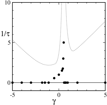
This symmetric quadratic form is simple enough that its eigenvalues and eigenvectors can be determined analytically . All of these eigenvalues depend on the two dynamical parameters $\{\zeta,\gamma\}$ but not on any of the kinematical parameters. The maximum eigenvalue also depends on position in Rindler space, according to ${\bar{\lambda}}_{\max}=f(\zeta,\gamma)+4x^{2}$, where $x$ is the Rindler coordinate. This eigenvalue has the (approximate) minimum value ${\bar{\lambda}}_{\max}^{2}=10.198+4x^{2}$ at the point $\{\zeta,\gamma\}=\{-0.135,-1.382\}$. In our growth rate estimates we evaluate the eigenvalue at the point in our computational domain where ${\bar{\lambda}}_{\max}$ has its maximum value, which in our case is at $x=1$.

Figure 3: Solid curve shows (half) the largest eigenvalue of $\bar{C}_{\alpha\beta}$ for the Rindler spacetime (with $k_{n}=0$). Dots give values for the actual growth rate of the short timescale instability as determined by numerical solution of the linearized evolution equations with $\zeta=-1$.

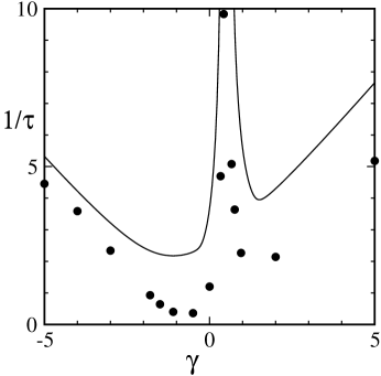
We illustrate in Fig. 3 the dependence of ${\scriptstyle\frac{1}{2}}{\bar{\lambda}}_{\max}$ on the parameter $\gamma$ (for $\zeta=-1$). Our simple analysis predicts that the best-behaved form of the evolution equations should be obtained for parameter values near this minimum. We also plot in Fig. 3 numerically-determined points that represent the growth rates of the instability. These points were evaluated from the growth rate of the energy norm for evolutions of the linearized KST equations using a 1D pseudospectral method on the domain $x\in[0.1,1]$. The numerical method (but not the system of equations) is identical to the one described in Kidder et al. (2000), except here our spatial coordinate is the Cartesian coordinate $x$ rather than the spherical coordinate $r$. All evolutions are performed at multiple resolutions (see Fig. 4) to test convergence, and the growth rates that we quote in the text and in the figures are taken from the converged solution. At the boundaries we demand that incoming characteristic fields have zero time derivative, and we do not constrain the outgoing and nonpropagating characteristic fields. The initial data is taken to be the exact solution plus a perturbation of the form $Ae^{-(x-0.55)^{2}/w^{2}}$ that is added to each of the dynamical variables ($g_{ij}$,$K_{ij}$,$M_{kij}$). The perturbation amplitude $A$ for each variable is a randomly chosen number in the interval $(-10^{-8},10^{-8})$. Note that this perturbation violates the constraints. The gauge fields $\beta^{i}$ and $Q$ are not perturbed. We measure the growth rates of the energy norm during the very earliest parts of the evolutions, before the initial Gaussian pulse can propagate to the edge of the computational domain. To do this we use an extremely narrow pulse $w=0.0125$, so that there is sufficient time to measure the growth rate before even the tail of the pulse reaches the boundary (one could also widen the computational domain, but this is equivalent to changing the pulse width because the Rindler solution is scale-invariant).

Figure 3 illustrates that the analytical estimate consisting of $1/\tau\approx{\scriptstyle\frac{1}{2}}{\bar{\lambda}}_{\max}$ gives a reasonably good estimate of this initial growth rate of the instability. And the location of the optimal value of the parameter $\gamma$, where the growth rate of the instability is minimum, also agrees fairly well with the location of the minimum of ${\scriptstyle\frac{1}{2}}{\bar{\lambda}}_{\max}$.

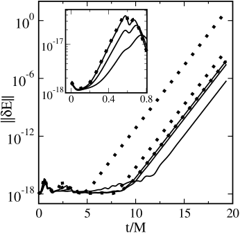
However, the short timescale instabilities illustrated in Fig. 3 are not our primary concern here. Figure 4 illustrates the evolution of the energy norm for one of the evolutions discussed above (with $\gamma=\frac{1}{3}$, $\zeta=-1$, $w=0.025$). This shows that once the unstable initial pulse crosses and leaves the computational domain (in about half a light crossing time, or $t\sim 0.6$), the solution grows much less rapidly. While the short term instability does not seriously effect the long term stability of the code (unless it is large enough that the code blows up in less than a crossing time), Fig. 4 illustrates that there are often other instabilities that grow more slowly, but which can contaminate and eventually destroy any attempts to integrate the equations for long periods of time. Figure 4 also illustrates the equivalence between evolving the system using a 1+1 dimensional finite difference code and a pseudo-spectral code. The finite difference code uses a first-order upwind method (see, e.g.  Leveque (1992)) in which the fundamental variables are decomposed into characteristic fields. Both the finite difference and the pseudo-spectral methods use the same initial data, boundary conditions, and gauge conditions. Three different spatial resolutions are illustrated for each method, and the highest resolution runs essentially coincide. This agreement provides additional evidence that the instabilities discussed here are features of the analytical evolution equations, and are not numerical in origin.

Figure 4: Evolution of the energy norm for perturbations of Rindler space. The solid curves show the evolutions based on a three different resolutions (101, 401 and 6401 grid points) of a finite difference version of the code, while dotted curves show the same evolution using three different spectral resolutions (64, 96, and 128 basis functions). A magnified view of the first part of the evolution (upper left) illustrates the short timescale instability whose growth rate is shown in Fig. 3.

In our estimates, we will now attempt to filter out the less interesting short term instabilities by imposing boundary conditions on the trial eigenfunctions $\delta u^{\alpha}$ used in Eq. (14). These boundary conditions are implemented using the projection operator $P^{\mu}{}_{\nu}$ in Eq. (16). For the case of the Rindler geometry this projection operator is constructed to annihilate both the ingoing and outgoing propagating modes. Thus the growth rate estimate given in Eq. (18) is implemented by finding the largest eigenvalue of $\bar{C}_{\alpha\beta}P^{\alpha}{}_{\mu}P^{\beta}{}_{\nu}$ that is projected onto the subspace of non-propagating modes (i.e. the eigenvectors of $\hat{x}_{k}A^{k\alpha}{}_{\beta}$ having eigenvalue zero, as measured by a hypersurface orthogonal observer). We find that the largest eigenvalue of this $\bar{C}_{\alpha\beta}P^{\alpha}{}_{\mu}P^{\beta}{}_{\nu}$ is zero for all values of $\{\zeta,\gamma\}$, for all values of the wavevector $k_{n}$, and for all values of $x$: the non-propagating modes of Rindler are all stable according to this estimate.

Figure 5: Solid curve illustrates the simple analytical growth rate estimate $1/\tau=0$ for the Rindler spacetime. Points are growth rates determined numerically for long-term (many light crossing times) evolutions with $\zeta=-1$. Dotted curve represents the short-term instability growth rate estimate.

This estimate of the long-term growth rate in Rindler is shown as the solid curve in Fig. 5. The points in Fig. 5 represent growth rates determined numerically over many many light crossing times (for these evolutions, we have no need for an extremely narrow pulse; we use $w=0.1$ so that we can run at lower resolutions). We observed that these equations are in fact stable for most values of the parameter $\gamma$ over these timescales. The only long term instabilities that we observed in Rindler occur for values of $\gamma$ near 0.5, where the short-term instability growth rate is infinite. We believe these instabilities occur because of coupling in the evolution equations between the pure propagating and non-propagating modes used in our simple estimate.

IV.2 Schwarzschild Spacetime

We have also studied instabilities in the Einstein evolution equations for solutions that are close to the Schwarzschild geometry. We use the Painlevé-Gullstrand Painlevé (1921); Gullstrand (1922); Martel and Poisson (2001) form of the Schwarzschild metric:

$$ds^{2}=-dt^{2}+\left(dr+\sqrt{2M/r}dt\right)^{2}+r^{2}d\Omega^{2},$$ (109)

where $d\Omega^{2}$ represents the standard metric on the unit sphere. The dynamical fields that represent this geometry are also quite simple (although not quite as simple as Rindler). In Cartesian coordinates we have

$$g_{ij} = \delta_{ij},$$ (110)

$$K_{ij} = \sqrt{2M/r^{3}}\delta_{ij}-3\sqrt{M/2r^{3}}\hat{r}_{i}\hat{r}_{j},$$ (111)

$$D_{kij} = 0,$$ (112)

$$N = 1,$$ (113)

$$N^{k} = \sqrt{2M/r}\hat{r}^{k},$$ (114)

where $\delta_{ij}$ is the Euclidean metric (in Cartesian coordinates), and $\hat{r}^{k}=(x,y,z)/r$ is the unit vector in the radial direction. In this representation of the Schwarzschild geometry the fundamental representation of the dynamical fields $u^{\alpha}_{0}=\{\delta_{ij},K_{ij},0\}$ includes a non-vanishing extrinsic curvature. Therefore $\partial_{\mu}T^{\alpha}{}_{\beta}u^{\beta}_{0}$ will be non-zero for this geometry. Since the $D_{kij}$ components of $u^{\alpha}_{0}$ are still zero, it follows that only the $K_{ij}$ components of $T^{\alpha}{}_{\beta}$ will contribute to $V^{\mu}{}_{\alpha}$. One can show that only the $K_{ij}$ components of $V^{\mu}{}_{\alpha}\delta u^{\alpha}_{0}$ are non-zero, and that these are given by:

$$\frac{\hat{z}}{1+3\hat{z}}\left[(1+3\hat{z})K\delta^{a}_{i}\delta^{b}_{j}-\hat{z}Kg_{ij}g^{ab}-g_{ij}K^{ab}\right]\delta g_{ab}.$$ (115)

Thus $V^{\mu}{}_{\alpha}$ depends only on the kinematical parameter $\hat{z}$. Consequently for evolutions near the representation of the Schwarzschild geometry considered here, the growth rates of the instabilities will depend on only three of the nine KST parameters: $\{\zeta,\gamma,\hat{z}\}$.

We solve the evolution equations for the perturbed Schwarzschild geometry using a pseudospectral collocation method (see, e.g. Boyd (1989); Canuto et al. (1988) for a general review, and Kidder et al. (2000, 2001, ) for more details of the particular implementation used here) on a 3D spherical-shell domain extending from $r=1.9M$ to $r=11.9M$. Our code utilizes the method of lines; the time integration is performed using a fourth order Runge-Kutta algorithm. The inner boundary lies inside the event horizon; at this boundary all characteristic curves are directed out of the domain (into the black hole), so no boundary condition is required there and none is imposed (“horizon excision” Seidel and Suen (1992); Alcubierre and Schutz (1994); Anninos et al. (1995); Gundlach and Walker (1999); Scheel et al. (1997, 1995a, 1995b); Cook et al. (1998); Brandt et al. (2000); Alcubierre and Brügmann (2001); Alcubierre et al. (2001); Kidder et al. (2001)). This reflects the causality condition that the interior of a black hole cannot influence the exterior region. At the outer boundary we require that all ingoing characteristic fields be time-independent, but we allow all outgoing characteristic fields to propagate freely. The initial data is the exact solution Eqs. (110) through (114), plus a perturbation of the form $Ae^{-(r-7M)^{2}/4M^{2}}$ added to each of the 30 dynamical variables (the Cartesian components of $g_{ij}$, $K_{ij}$, and $M_{kij}$). The perturbation amplitude $A$ for each variable is a randomly chosen number in the interval $(-10^{-8},10^{-8})$. The gauge fields $\beta^{i}$ and $Q$ are not perturbed. Because we perturb the Cartesian components of each field by a spherically symmetric function, the initial data are not spherically symmetric. Note that we have chosen an initial perturbation that violates the constraints.

Figure 6: Dashed curve illustrates the simple analytical growth rate estimate for the Schwarzschild spacetime with $k_{n}=0$, and the solid curve shows estimate for $k_{n}=-\hat{r}_{n}/M$. Points are growth rates determined numerically for long-term (many light crossing times) evolutions of the 3D linearized equations with $\zeta=-1$ and $\hat{z}=-1/4$.

Figure 7: Same information as Fig. 6 but plotted here using a logarithmic scale. This illustrates that while the simple analytical growth rate estimate is qualitatively correct, it fails to correctly identify the optimum choice of parameters.

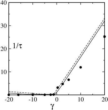
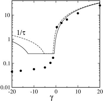
At the outer boundary, the modes that appear non-propagating to a hypersurface orthogonal observer actually are incoming with respect to the boundary because of the outward-directed radial shift vector $N^{i}$. Thus the projection operator $P^{\mu}{}_{\nu}$ needed to construct our growth rate estimates from Eq. (18) is therefore the one that annihilates both the incoming and the “non-propagating” modes, but leaves the outgoing modes unchanged. We have computed the eigenvalues of this appropriately projected $\bar{C}_{\alpha\beta}$, and illustrate the largest eigenvalue in Fig. 6. These eigenvalues depend on the radial coordinate $r$ in this spacetime, and we plot in Fig. 6 the largest value of this eigenvalue, which occurs at $r=2M$. The graph represents (half) this largest eigenvalue as a function of the parameter $\gamma$ for $\zeta=-1$ and $\hat{z}=-1/4$. In Fig. 6 we give estimates for two choices of the wavevector $k_{a}$ that characterizes the spatial variation of $\delta u^{\alpha}$: the dashed curve represents the choice $k_{n}=0$, while the solid curve represents the choice $k_{n}=-\hat{r}_{n}/M$. The points in this graph represent the numerically-determined growth rates of the instabilities for the linearized equations. We see that the agreement with our very simple analytical estimate is again quite good. However, Fig. 7 illustrates that while the simple analytical estimate is correct qualitatively, it fails to correctly identify the best choice of parameters to use for long-term numerical evolutions. The minimum growth rate is actually smaller (by about a factor of two) than what could be achieved by the optimal range of parameters that are identified by the simple analytical growth rate estimate.

Figure 8: Dashed curve illustrates the simple analytical growth rate estimate for the Schwarzschild spacetime with $k_{n}=0$, and the solid curve shows the estimate for $k_{n}=-\hat{r}_{n}/M$. Points are growth rates determined numerically for long-term (many light crossing times) 3D evolutions with $\zeta=-1$ and $\gamma=-16$.

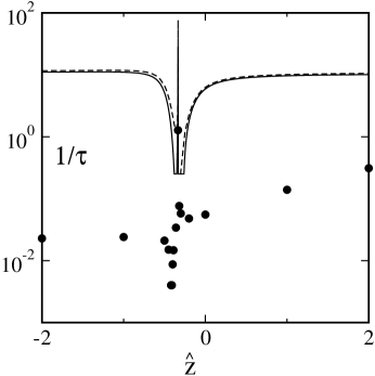
Fig. 8 is the same as Fig. 7 except the results are plotted as a function of the parameter $\hat{z}$ for $\zeta=-1$ and $\gamma=-16$. Again, the actual minimum growth rate is smaller than the analytical estimate. However, the qualitative shape of the analytical curve is correct, and can be used as a guide for choosing parameters to investigate with the numerical code. In the present case this guide proves extremely useful, for it has allowed us to find a parameter choice ($\hat{z}=-0.42$, $\gamma=-16$, $\zeta=-1$) that significantly extends the amount of time the fully 3D nonlinear code can evolve a single Schwarzschild black hole. The very narrow range of parameters where the evolution equations have optimal stability, as shown in Fig. 8, illustrate why these optimal values were not discovered empirically Kidder et al. (2001). The growth rate estimates derived here were needed to focus the search onto the relevant part of the parameter space. The improvement in 3D nonlinear black hole evolutions resulting from these better parameter choices will be discussed in detail in a forthcoming paper.

V Discussion

This paper studies the constraint-violating and gauge instabilities of the Einstein evolution equations. We derive an analytical expression for the growth rate of an energy norm in Sec. II. This energy norm measures the deviations of a given solution from a background constraint-satisfying solution. We show numerically that the growth rate of this energy norm is identical to the growth rate of constraint violations in solutions of both the linearized equations and of the full nonlinear equations. Thus we concentrate here on the analysis of the evolution of this energy norm. Section III derives the analytical expressions needed to evaluate this energy norm in the 12-parameter family of Einstein evolution equations introduced by Kidder, Scheel, and Teukolsky Kidder et al. (2001). This analysis demonstrates that an open subset of the KST equations with all physical characteristic speeds is symmetric hyperbolic. And perhaps more surprisingly, there is a large open subset of these strongly hyperbolic equations that is not symmetric hyperbolic.

We make a considerable effort in this paper to demonstrate that the instabilities that we observe are actual solutions to the evolution equations and not numerical artifacts of the discrete representation of the solution that we use. We run many of the cases that we study here using both a finite difference and a pseudo-spectral version of the code, and find equivalent results. We run all numerical simulations at multiple spatial and temporal resolutions to demonstrate that numerical convergence to the desired accuracy is achieved. We also confirm that the growth rate determined from our analytical integral expression is equal (to the desired numerical accuracy) to the growth rate measured numerically from the growth of the energy norm. This equality is expected only for solutions to the actual evolution equations, so this provides a non-trivial check that the instabilities we find are real solutions to the equations.

The analysis presented here also suggests that the instabilities that we see are endemic to the Einstein evolution equations and are not the result of improper boundary conditions. We impose conditions that suppress the incoming components of the dynamical fields at the boundaries of the computational domain. These conditions (sometimes called maximally dissipative Szilágyi and Winicour (2002)) ensure that the energy norm does not grow due to energy being inserted into the computational domain across the boundaries. Any other boundary conditions that might be imposed (including ones that attempt to control the influx of constraint violations Calabrese et al. (2001)) could only increase the growth rate of our energy norm. Because the constraint violations grow at the same rate as the energy norm, it seems very unlikely that the constraint violations could be eliminated or even significantly reduced simply by changing the boundary conditions. And even if the constraint violations could be eliminated with better boundary conditions, our analysis shows that something—presumably gauge instabilities—would still cause the energy norms to grow on the timescales illustrated here.

The analysis presented here provides additional support for the claim that the growth rate of instabilities is strongly affected by the choice of representation of the Einstein evolution equations. We find that this growth rate varies considerably as the parameters in the KST formulation of the equations are varied. Further, we demonstrate here that the functional dependence of the growth rate on the parameters strongly depends on the initial data that are being evolved. We show that the functional dependence on the set of parameters is not the same for the Schwarzschild geometry as it is for flat spacetime in Rindler coordinates. This result strongly suggests that analyzing the stability of the evolution equations for perturbations of flat spacetime in Minkowski coordinates Alcubierre et al. (2000b); Yoneda and Shinkai (2002), although useful for screening out particularly poorly-behaved formulations, is unlikely to succeed in identifying the best form of the equations to use for binary black hole spacetime evolutions. Rather these results suggest that it may be necessary to choose the optimal form of the evolution equations individually for each problem. Estimates of the instability growth rates such as those found here (and hopefully more refined estimates yet to be discovered) depend only on the fields at a given instant of time. It might be possible (or even necessary) then to use such estimates to determine and then adjust the form of the evolution equations to be optimal as the spacetime evolves.

Appendix A

In this Appendix we give the details of a number of equations that define the KST Kidder et al. (2001) formulation of the Einstein evolution equations. The principal parts of these equations can be written in the form of a first order system:

$$\partial_{t}u^{\alpha}+A^{k\alpha}{}_{\beta}\partial_{k}u^{\beta}\simeq 0.$$ (116)

Here the dynamical fields are taken to be the set $u^{\alpha}=\{g_{ij},P_{ij},M_{kij}\}$, where $g_{ij}$ is the spatial metric, and $P_{ij}$ and $M_{kij}$ are fields that initially will be interpreted as the extrinsic curvature $K_{ij}$ and the spatial derivatives of the metric $D_{kij}={\scriptstyle\frac{1}{2}}\partial_{k}g_{ij}$ respectively. The matrices $A^{k\alpha}{}_{\beta}$ can be written quite generally for these systems in the form

$$\partial{}_{t}g{}_{ij} \simeq N^{n}\partial_{n}g_{ij},$$ (117)

$$\partial{}_{t}P{}_{ij} \simeq N^{n}\partial_{n}K_{ij}-N\Bigl{[}\mu{}_{1}g{}^{nb}\delta{}^{c}{}_{i}\delta{}^{d}{}_{j}+\mu{}_{2}g{}^{nd}\delta{}^{b}{}_{(i}\delta{}^{c}{}_{j)}$$ (118)

$$+\mu{}_{3}g{}^{bc}\delta{}^{n}{}_{(i}\delta{}^{d}{}_{j)}+\mu{}_{4}g{}^{cd}\delta{}^{n}{}_{(i}\delta{}^{b}{}_{j)}$$

$$+\mu{}_{5}g{}^{nd}g{}^{bc}g{}_{ij}+\mu{}_{6}g{}^{nb}g{}^{cd}g{}_{ij}\Bigr{]}\partial{}_{k}M{}_{bcd},$$

$$\partial{}_{t}M{}_{kij} \simeq N^{n}\partial_{n}M_{kij}-N\Bigl{[}\nu{}_{1}\delta{}^{n}{}_{k}\delta{}^{b}{}_{i}\delta{}^{c}{}_{j}+\nu{}_{2}\delta{}^{n}{}_{(i}\delta{}^{b}{}_{j)}\delta{}^{c}{}_{k}$$ (119)

$$+\nu{}_{3}g{}^{nb}g{}_{k(i}\delta{}^{c}{}_{j)}+\nu{}_{4}g{}^{nb}g{}_{ij}\delta{}^{c}{}_{k}$$

$$+\nu{}_{5}g{}^{bc}g{}_{k(i}\delta{}^{n}{}_{j)}+\nu{}_{6}g{}^{bc}g{}_{ij}\delta{}^{n}{}_{k}\Bigr{]}\partial{}_{n}P{}_{bc}.$$

For the fundamental representations of the theory discussed in Sec. III where the dynamical fields are $u^{\alpha}_{0}=\{g_{ij},K_{ij},D_{kij}\}$, the constants $\mu_{A}$ and $\nu_{A}$ are related to the 5 dynamical KST parameters $(\gamma,\zeta,\eta,\chi,\sigma)$ by,

$$\mu_{1} = \nu_{1}=1,$$ (120)

$$\mu_{2} = -1-\zeta,$$ (121)

$$\mu_{3} = -1+\zeta,$$ (122)

$$\mu_{4} = 1+2\sigma,$$ (123)

$$\mu_{5} = -\mu_{6}=-\gamma,$$ (124)

$$\nu_{2} = 0,$$ (125)

$$\nu_{3} = -\nu_{5}=-{\scriptstyle\frac{1}{2}}\eta,$$ (126)

$$\nu_{4} = -\nu_{6}=-{\scriptstyle\frac{1}{2}}\chi.$$ (127)

KST Kidder et al. (2001) generalize this fundamental representation of the theory by introducing a 7-parameter family of transformations on the dynamical fields. These transformations define the new fields $P_{ij}$ and $M_{kij}$ in terms of the fundamental fields $K_{ij}$ and $D_{kij}$ via an equation of the form

$$u^{\alpha}=T^{\alpha}{}_{\beta}u^{\beta}_{0}.$$ (128)

The explicit form of this transformation is given in Eqs. (30) and (31). Here we give explicit expressions for the inverse transformation:

$$K_{ij}=P_{ij}+\bar{z}\,g_{ij}g^{ab}P_{ab},$$ (129)

$$D_{kij}=\bigl{[}\bar{k}\,\delta{}^{a}_{k}\delta{}^{b}_{i}\delta{}^{c}_{j}+\bar{e}\,\delta{}^{a}_{(i}\delta{}^{b}_{j)}\delta{}^{c}_{k}+\bar{a}\,g{}_{ij}g^{bc}\delta{}^{a}_{k}\qquad\qquad$$

$$\quad\qquad+\bar{b}\,g{}_{ij}g^{ab}\delta{}^{c}_{k}+\bar{c}\,g{}_{k(i}\delta{}^{a}_{j)}g^{bc}+\bar{d}\,g{}_{k(i}\delta{}^{c}_{j)}g^{ab}\bigr{]}M_{abc},$$

(130)

where the constants $\{\bar{z},\bar{k},\bar{a},\bar{b},\bar{c},\bar{d},\bar{e}\}$ are functions of the kinematical parameters $\{\hat{z},\hat{k},\hat{a},\hat{b},\hat{c},\hat{d},\hat{e}\}$:

$$\bar{z} = -\hat{z}/(1+3\hat{z}),$$ (131)

$$\delta\bar{a} = 2(3\hat{e}+4\hat{k})(\hat{b}\hat{c}-\hat{a}\hat{d})-(\hat{a}-\hat{b}-\hat{c}+\hat{d})\hat{e}^{2}\qquad$$ (132)

$$\qquad\qquad-2(2\hat{a}\hat{e}-\hat{b}\hat{e}-\hat{c}\hat{e}+2\hat{a}\hat{k})\hat{k},\qquad$$

$$\delta\bar{b} = 4(2\hat{e}+\hat{k})(\hat{a}\hat{d}-\hat{b}\hat{c})+2(\hat{a}-\hat{c})\hat{e}^{2}$$ (133)

$$\qquad\qquad+2(2\hat{a}\hat{e}-\hat{b}\hat{e}+\hat{d}\hat{e}-2\hat{b}\hat{k})\hat{k},\qquad$$

$$\delta\bar{c} = 4(2\hat{e}+\hat{k})(\hat{a}\hat{d}-\hat{b}\hat{c})+2(\hat{a}-\hat{b})\hat{e}^{2}$$ (134)

$$\qquad\qquad+2(2\hat{a}\hat{e}-\hat{c}\hat{e}+\hat{d}\hat{e}-2\hat{c}\hat{k})\hat{k},\qquad$$

$$\delta\bar{d} = 4(\hat{e}+3\hat{k})(\hat{b}\hat{c}-\hat{a}\hat{d})-4\hat{a}\hat{e}^{2}$$ (135)

$$\qquad\qquad+4(\hat{b}\hat{e}+\hat{c}\hat{e}-\hat{d}\hat{k})\hat{k},\qquad$$

$$\delta_{0}\bar{e} = 2\hat{e},$$ (136)

$$\delta_{0}\bar{k} = -\hat{e}-2\hat{k},$$ (137)

$$\delta_{0} = \hat{e}^{2}-\hat{e}\hat{k}-2\hat{k}^{2},$$ (138)

$$\delta = \delta_{0}\bigl{[}10(\hat{b}\hat{c}-\hat{a}\hat{d})+(3\hat{b}+3\hat{c}-\hat{a}+\hat{d}+\hat{e})\hat{e}$$ (139)

$$\qquad-(6\hat{a}+2\hat{b}+2\hat{c}+4\hat{d}+\hat{e}+2\hat{k})\hat{k}\bigr{]}.$$

The transformation $T^{\alpha}{}_{\beta}$ is invertible as long as $\delta\neq 0$ and $\hat{z}\neq-{\scriptstyle\frac{1}{3}}$. In this generic case we may write

$$u^{\alpha}_{0}=T^{-1\,\alpha}{}_{\beta}u^{\beta},$$ (140)

and $T^{\alpha}{}_{\gamma}T^{-1\,\gamma}{}_{\beta}=\delta^{\alpha}{}_{\beta}$, where $\delta^{\alpha}{}_{\beta}$ is the identity matrix on the space of fields.

We have seen in Sec. III that the general expression for the matrices $A^{k\alpha}{}_{\beta}$ is related to its form in the fundamental representation of the equations, $A^{k}_{0}{}^{\alpha}{}_{\beta}$, by the simple transformation law: $A^{k\alpha}{}_{\beta}=T^{\alpha}{}_{\mu}A^{k}_{0}{}^{\mu}{}_{\nu}T^{-1\,\nu}{}_{\beta}$. This transformation may also be expressed somewhat more concretely as a transformation on the constants $\mu_{A}$ and $\nu_{A}$ that define the matrices $A^{k\alpha}{}_{\beta}$. The resulting expressions for these constants after the kinematical transformation are:

$$\mu_{1} = \bar{k}-{\scriptstyle\frac{1}{2}}(1+\zeta)\bar{e},$$ (141)

$$\mu_{2} = {\scriptstyle\frac{1}{2}}(1-\zeta)\bar{e}-(1+\zeta)\bar{k},$$ (142)

$$\mu_{3} = (1+6\sigma)\bar{b}-(1-\zeta)\bar{k}-{\scriptstyle\frac{1}{2}}(1-4\sigma-3\zeta)\bar{d}$$ (143)

$$+{\scriptstyle\frac{1}{2}}(1+4\sigma+\zeta)\bar{e},$$

$$\mu_{4} = (1+6\sigma)\bar{a}+(1+2\sigma)\bar{k}-{\scriptstyle\frac{1}{2}}(1-4\sigma-3\zeta)\bar{c}$$ (144)

$$-{\scriptstyle\frac{1}{2}}(1-\zeta)\bar{e},$$

$$\mu_{5} = (1+2\gamma+4\hat{z}+6\gamma\hat{z})(\bar{b}-{\scriptstyle\frac{1}{2}}\bar{d})+2\sigma\hat{z}(3\bar{b}+\bar{d}+\bar{e})$$ (145)

$$-(\gamma+2\hat{z}+3\gamma\hat{z})(\bar{k}-{\scriptstyle\frac{1}{2}}\bar{e})-{\scriptstyle\frac{1}{2}}\zeta\bar{d},$$

$$\mu_{6} = (1+2\gamma+4\hat{z}+6\gamma\hat{z})(\bar{a}-{\scriptstyle\frac{1}{2}}\bar{c})+2\sigma\hat{z}(3\bar{a}+\bar{k}+\bar{c})$$ (146)

$$+(\gamma+2\hat{z}+3\gamma\hat{z})(\bar{k}-{\scriptstyle\frac{1}{2}}\bar{e})-{\scriptstyle\frac{1}{2}}\zeta\bar{c},$$

$$\nu_{1} = \hat{k},$$ (147)

$$\nu_{2} = \hat{e},$$ (148)

$$\nu_{3} = (1-\eta-{\scriptstyle\frac{1}{2}}\chi)\hat{d}-{\scriptstyle\frac{1}{2}}(\eta+3\chi)\hat{c}-{\scriptstyle\frac{1}{4}}(\eta+2\chi)\hat{e}-{\scriptstyle\frac{1}{2}}\eta\hat{k},$$

$$\nu_{4} = (1-\eta-{\scriptstyle\frac{1}{2}}\chi)\hat{b}-{\scriptstyle\frac{1}{2}}(\eta+3\chi)\hat{a}-{\scriptstyle\frac{1}{4}}\eta\hat{e}-{\scriptstyle\frac{1}{2}}\chi\hat{k},$$ (150)

$$\nu_{5} = {\scriptstyle\frac{1}{2}}(2+\eta+3\chi+6\bar{z}+2\eta\bar{z}+6\chi\bar{z})\hat{c}$$ (151)

$$+{\scriptstyle\frac{1}{2}}(2\eta+\chi+2\bar{z}+4\eta\bar{z}+2\chi\bar{z})\hat{d}+{\scriptstyle\frac{1}{2}}(\eta+2\eta\bar{z})\hat{k}$$

$$+{\scriptstyle\frac{1}{4}}(\eta+2\chi+4\bar{z}+2\eta\bar{z}+4\chi\bar{z})\hat{e},$$

$$\nu_{6} = {\scriptstyle\frac{1}{2}}(2+\eta+3\chi+6\bar{z}+2\eta\bar{z}+6\chi\bar{z})\hat{a}$$ (152)

$$+{\scriptstyle\frac{1}{2}}(2\eta+\chi+2\bar{z}+4\eta\bar{z}+2\chi\bar{z})\hat{b}$$

$$+{\scriptstyle\frac{1}{4}}(\eta+2\eta\bar{z})\hat{e}+{\scriptstyle\frac{1}{2}}(\chi+2\bar{z}+2\chi\bar{z})\hat{k}.$$

These expressions are identical to those in KST Kidder et al. (2001) except for $\mu_{5}$ and $\mu_{6}$, which differ from the the KST expressions (due to a typographical error in KST) by the substitutions $\bar{c}\leftrightarrow\bar{d}$.

Finally we wish to give an explicit expression for the transformation that relates a fundamental representation of the symmetrizer $S^{0}_{\alpha\beta}$ with the general representation $S_{\alpha\beta}$. We have seen in Sec. III.2 that a symmetrizer $S_{\alpha\beta}$ is determined by a set of constants $B_{A}$ and $C_{A}$, and similarly the fundamental representation $S^{0}_{\alpha\beta}$ is determined by constants $B^{0}_{A}$ and $C^{0}_{A}$. The general symmetrizer is related to the fundamental by Eq. (58), $S_{\alpha\beta}=T^{-1\mu}{}_{\alpha}S^{0}_{\mu\nu}T^{-1\nu}{}_{\beta}$. This transformation can be represented more concretely as relationships between the constants $B_{A}$ and $C_{A}$ that define $S_{\alpha\beta}$ and the constants $B^{0}_{A}$ and $C^{0}_{A}$ that define $S^{0}_{\alpha\beta}$. These relations are:

$$B_{1} = (1+3\bar{z})^{2}B_{1}^{0},$$ (153)

$$B_{2} = B_{2}^{0},$$ (154)

$$C_{1} = (\bar{k}+\bar{e})^{2}C_{1}^{0},$$ (155)

$$C_{2} = (\bar{k}-{\scriptstyle\frac{1}{2}}\bar{e})^{2}C_{2}^{0},$$ (156)

$$C_{3} = {\cal A}^{2}C_{3}^{0}+{\cal B}^{2}C_{4}^{0}+2{\cal AB}C_{5}^{0},$$ (157)

$$C_{4} = {\cal D}^{2}C_{3}^{0}+{\cal E}^{2}C_{4}^{0}+2{\cal DE}C_{5}^{0},$$ (158)

$$C_{5} = {\cal AD}C_{3}^{0}+{\cal BE}C_{4}^{0}+({\cal AE+BD})C_{5}^{0},$$ (159)

where

$${\cal A} = \bar{k}+3\bar{a}+\bar{c},$$ (160)

$${\cal B} = {\scriptstyle\frac{1}{2}}\bar{e}+\bar{a}+2\bar{c},$$ (161)

$${\cal D} = \bar{e}+3\bar{b}+\bar{d},$$ (162)

$${\cal E} = \bar{k}+{\scriptstyle\frac{1}{2}}\bar{e}+\bar{b}+2\bar{d}.$$ (163)

It is straightforward to verify that these $B_{A}$ and $C_{A}$ satisfy the positivity conditions needed to guarantee that $S_{\alpha\beta}$ is positive definite, so long as the $B^{0}_{A}$ and $C^{0}_{A}$ also satisfy those conditions.

References

- Arnowitt et al. (1962) R. Arnowitt, S. Deser, and C. W. Misner, in Gravitation: An Introduction to Current Research, edited by L. Witten (Wiley, New York, 1962), pp. 227–265.
- York (1979) J. W. York, Jr., in Sources of Gravitational Radiation, edited by L. L. Smarr (Cambridge University Press, Cambridge, England, 1979), pp. 83–126.
- Shibata and Nakamura (1995) M. Shibata and T. Nakamura, Phys. Rev. D 52, 5428 (1995).
- Baumgarte and Shapiro (1999) T. W. Baumgarte and S. L. Shapiro, Phys. Rev. D 59, 024007 (1999).
- Fischer and Marsden (1979) A. E. Fischer and J. E. Marsden, in General Relativity: An Einstein Centenary Survey, edited by S. W. Hawking and W. Israel (Cambridge University Press, Cambridge, England, 1979), pp. 138–211.
- Bona and Massó (1992) C. Bona and J. Massó, Phys. Rev. Lett. 68, 1097 (1992).
- Frittelli and Reula (1994) S. Frittelli and O. Reula, Commun. Math. Phys. 166, 221 (1994).
- Bona et al. (1995) C. Bona, J. Massó, E. Seidel, and J. Stela, Phys. Rev. Lett. 75, 600 (1995).
- Choquet-Bruhat and York (1995) Y. Choquet-Bruhat and J. W. York, Jr., C. R. Acad. Sci., Ser. 1 A321, 1089 (1995).
- Abrahams et al. (1995) A. Abrahams, A. Anderson, Y. Choquet-Bruhat, and J. W. York, Jr., Phys. Rev. Lett. 75, 3377 (1995).
- van Putten and Eardley (1996) M. H. P. M. van Putten and D. M. Eardley, Phys. Rev. D 53, 3056 (1996).
- Frittelli and Reula (1996) S. Frittelli and O. A. Reula, Phys. Rev. Lett. 76, 4667 (1996).
- Friedrich (1996) H. Friedrich, Class. Quantum Grav. 13, 1451 (1996).
- Estabrook et al. (1997) F. B. Estabrook, R. S. Robinson, and H. D. Wahlquist, Class. Quantum Grav. 14, 1237 (1997).
- Iriondo et al. (1997) M. S. Iriondo, E. O. Leguizamon, and O. A. Reula, Phys. Rev. Lett. 79, 4732 (1997).
- Anderson et al. (1997) A. Anderson, Y. Choquet-Bruhat, and J. W. York, Jr., Topol. Meth. Nonlin. Anal. 10, 353 (1997).
- Bonilla (1998) M. A. G. Bonilla, Class. Quantum Grav. 15, 2001 (1998).
- Yoneda and Shinkai (1999) G. Yoneda and H. Shinkai, Phys. Rev. Lett. 82, 263 (1999).
- Anderson and York (1999) A. Anderson and J. W. York, Jr., Phys. Rev. Lett. 82, 4384 (1999).
- Frittelli and Reula (1999) S. Frittelli and O. A. Reula, J. Math. Phys. 40, 5143 (1999).
- Alcubierre et al. (1999) M. Alcubierre, B. Brügmann, M. Miller, and W.-M. Suen, Phys. Rev. D 60, 064017 (1999).
- Hern (1999) S. D. Hern, Ph.D. thesis, University of Cambridge (1999), gr-qc/0004036.
- Friedrich and Rendall (2000) H. Friedrich and A. Rendall, in Einstein’s Field Equations and their Physical Implications, edited by B. G. Schmidt (Springer-Verlag, Berlin, 2000), Lecture Notes in Physics, pp. 127–223.
- Yoneda and Shinkai (2000) G. Yoneda and H. Shinkai, Int. J. Mod. Phys. D 9, 13 (2000).
- Shinkai and Yoneda (2000) H. Shinkai and G. Yoneda, Class. Quantum Grav. 17, 4799 (2000).
- Kidder et al. (2001) L. E. Kidder, M. A. Scheel, and S. A. Teukolsky, Phys. Rev. D 64, 064017 (2001).
- Yoneda and Shinkai (2001) G. Yoneda and H. Shinkai, Class. Quantum Grav. 18, 441 (2001).
- Shinkai and Yoneda (2002) H. Shinkai and G. Yoneda, Class. Quantum Grav. 19, 124019 (2002).
- Alvi (2002) K. Alvi, First-order symmetrizable hyperbolic formulations of einstein’s equations including lapse and shift as dynamical fields (2002), eprint gr-qc/0204068.
- Sarbach and Tiglio (2002) O. Sarbach and M. Tiglio, Exploiting gauge and constraint freedom in hyperbolic formulations of einstein’s equations (2002), eprint gr-qc/0205086.
- Yoneda and Shinkai (2002) G. Yoneda and H. Shinkai, Advantages of modified adm formulation: constraint propagation analysis of Baumgarte-Shapiro-Shibata-Nakamura system (2002), eprint gr-qc/0204002.
- Laguna and Shoemaker (2002) P. Laguna and D. Shoemaker, Numerical stability of a new conformal-traceless 3+1 formulation of the Einstein equation, gr-qc/0202105 (2002).
- Scheel et al. (1998) M. A. Scheel, T. W. Baumgarte, G. B. Cook, S. L. Shapiro, and S. A. Teukolsky, Phys. Rev. D 58, 044020 (1998).
- Alcubierre et al. (2000a) M. Alcubierre, B. Brügmann, T. Dramlitsch, J. A. Font, P. Papadopoulos, E. Seidel, N. Stergioulas, and R. Takahashi, Phys. Rev. D 62, 044034 (2000a).
- Calabrese et al. (2002) G. Calabrese, J. Pullin, O. Sarbach, and M. Tiglio, Stability properties of a formulation of einstein’s equations (2002), eprint gr-qc/0205073.
- Alcubierre et al. (2000b) M. Alcubierre, G. Allen, B. Brügmann, E. Seidel, and W.-M. Suen, Phys. Rev. D 62, 124011 (2000b).
- Knapp et al. (2002) A. M. Knapp, E. J. Walker, and T. W. Baumgarte, prd 65, 064031 (2002).
- Wald (1984) R. M. Wald, General Relativity (University of Chicago Press, 1984).
- Painlevé (1921) P. Painlevé, Acad. Sci., Paris, C. R. 173, 677 (1921).
- Gullstrand (1922) A. Gullstrand, Ark. Mat. Astron. Fys. 16, 1 (1922).
- Martel and Poisson (2001) K. Martel and E. Poisson, Am. J. Phys. 69, 476 (2001).
- Kreiss and Lorenz (1989) H.-O. Kreiss and J. Lorenz, Initial-Boundary Value Problems and the Navier-Stokes Equations (Academic Press, San Diego, 1989).
- Courant and Hilbert (1962) R. Courant and D. Hilbert, Methods of Mathematical Physics, Vol. II (John Wiley and Sons, 1962).
- Gustafsson et al. (1995) B. Gustafsson, H.-O. Kreiss, and J. Oliger, Time Dependent Problems and Difference Methods, Pure and Applied Mathematics (Wiley, New York, 1995).
- Kidder et al. (2000) L. E. Kidder, M. A. Scheel, S. A. Teukolsky, E. D. Carlson, and G. B. Cook, Phys. Rev. D 62, 084032 (2000).
- Leveque (1992) R. J. Leveque, Numerical Methods for Conservation Laws (Birkhauser Verlag, Basel, 1992).
- Boyd (1989) J. P. Boyd, Chebyshev and Fourier Spectral Methods (Springer-Verlag, Berlin, 1989).
- Canuto et al. (1988) C. Canuto, M. Y. Hussaini, A. Quarteroni, and T. A. Zang, Spectral Methods in Fluid Dynamics (Springer-Verlag, Berlin, 1988).
- (49) L. E. Kidder, M. A. Scheel, H. P. Pfeiffer, and S. A. Teukolsky, in preparation.
- Seidel and Suen (1992) E. Seidel and W.-M. Suen, Phys. Rev. Lett. 69, 1845 (1992).
- Alcubierre and Schutz (1994) M. Alcubierre and B. F. Schutz, J. Comput. Phys. 112, 44 (1994).
- Anninos et al. (1995) P. Anninos, G. Daues, J. Massó, E. Seidel, and W.-M. Suen, Phys. Rev. D 51, 5562 (1995).
- Gundlach and Walker (1999) C. Gundlach and P. Walker, Class. Quantum Grav. 16, 991 (1999).
- Scheel et al. (1997) M. A. Scheel, T. W. Baumgarte, G. B. Cook, S. L. Shapiro, and S. A. Teukolsky, Phys. Rev. D 56, 6320 (1997).
- Scheel et al. (1995a) M. A. Scheel, S. L. Shapiro, and S. A. Teukolsky, Phys. Rev. D 51, 4208 (1995a).
- Scheel et al. (1995b) M. A. Scheel, S. L. Shapiro, and S. A. Teukolsky, Phys. Rev. D 51, 4236 (1995b).
- Cook et al. (1998) G. B. Cook, M. F. Huq, S. A. Klasky, M. A. Scheel, et al., Phys. Rev. Lett. 80, 2512 (1998).
- Brandt et al. (2000) S. Brandt, R. Correll, R. Gomez, M. Huq, P. Laguna, L. Lehner, P. Marronetti, R. A. Matzner, D. Neilsen, J. P. E. Schnetter, et al., Phys. Rev. Lett. 85, 5496 (2000).
- Alcubierre and Brügmann (2001) M. Alcubierre and B. Brügmann, Phys. Rev. D 63, 104006 (2001).
- Alcubierre et al. (2001) M. Alcubierre, B. Brügmann, D. Pollney, E. Seidel, and R. Takahashi, Phys. Rev. D 64, 061501 (2001).
- Szilágyi and Winicour (2002) B. Szilágyi and J. Winicour, Well-posed initial-boundary evolution in general relativity (2002), eprint gr-qc/0205044.
- Calabrese et al. (2001) G. Calabrese, L. Lehner, and M. Tiglio, Constraint-preserving boundary conditions in numerical relativity, gr-qc/0111003 (2001).