Poincaré ball embeddings of the optical geometry

Abstract

It is shown that optical geometry of the Reissner-Nordström exterior metric can be embedded in a hyperbolic space all the way down to its outer horizon. The adopted embedding procedure removes a breakdown of flat-space embeddings which occurs outside the horizon, at and below the Buchdahl-Bondi limit ($R/M=9/4$ in the Schwarzschild case). In particular, the horizon can be captured in the optical geometry embedding diagram. Moreover, by using the compact Poincaré ball representation of the hyperbolic space, the embedding diagram can cover the whole extent of radius from spatial infinity down to the horizon. Attention is drawn to advantages of such embeddings in an appropriately curved space: this approach gives compact embeddings and it distinguishes clearly the case of an extremal black hole from a non-extremal one in terms of topology of the embedded horizon.

1 Introduction

This paper introduces a new, simple and convenient way to discuss physics of spacetime near the black hole horizon in terms of the optical geometry embedded in a Poincaré ball. We do not report a progress in developing new physical ideas. Instead, the goal of the present paper is more modest and concentrated on a useful though quite inconventional embedding procedure.

Embedding of curved spaces and spacetimes in a Euclidean space with a higher number of dimensions is a well-known technique, so often used in general relativity that there is no need to recall its usefulness here [8]. The optical geometry is also useful, but perhaps less known. In a static spacetime, it is defined by a particular conformal rescaling of the three-dimensional geometry of space (i.e. a hypersurface orthogonal to timelike Killing trajectories) in such a way that light trajectories in space are geodesic lines [3]. Therefore, the geometry of space can be directly established in terms of measurements based solely on light tracing. This is a rather useful property of the optical geometry that has already been employed by numerous authors for remarkable simplifications of various arguments and calculations, ranging from gravitational wave modes trapped in super-compact stars [10] to origin of the Hawking radiation [2].

Not only are geodesic lines optically straight, but they are also inertially, dynamically and electrically straight and their direction agrees at each point with dynamical, inertial and electrical experiments (e.g., a gyroscope that moves along such a straight line does not precess). These properties follow from the rather remarkable fact that all the relevant equations – geodesic, Fermi-Walker, Maxwell, Abraham-Lorentz-Dirac, Klein-Gordon – when written in the 3+1 form of the optical geometry are found to be identical with the corresponding equations in Minkowski spacetime with a scalar field $\Phi$ (the gravitational potential). For these reasons the geometry of optical space offers simple explanations of several physical effects in strongly curved spacetimes that otherwise could appear unclear or even confusing. See ref. [1] for a general exposition of the properties of optical geometry, and ref. [9] for a thorough discussion and derivations.

The optical geometry of a given spacetime cannot, in general, be embedded in a Euclidean space all the way to the horizon because of two separate reasons: (i) the horizon is, obviously, at an infinite distance in the optical geometry based on light tracing; (ii) optical geometry has a negative curvature near the horizon. In this paper we show, by embedding the optical geometry in a Poincaré ball, how one can avoid both of these difficulties. The Poincaré ball embeddings show clearly the topology of the horizon of the black hole. This feature should be helpful in discussing the role of the horizon topology in the context of the Hawking radiation. Our embeddings illustrate in a striking way the passage from non-extremal to the extremal Reissner-Nordström hole. In particular, the special nature of the extremal Reissner-Nordström hole is clearly manifested in terms of a change in the topology of the horizon. This feature is of interest in the context of supersymmetric theories where the extremal black holes show up as supersymmetric configurations [6].

2 An embedding procedure

First, we briefly describe a way to embed a two-dimensional hypersurface of a static and spherically symmetric spacetime in the three-dimensional (curved) space of a Poincaré ball [4, 12]. While a traditional approach to visualization of spherically symmetric geometries employs a direct embedding in the flat Euclidean space ${\mathbb{E}}^{3}$, the present method does not suffer from several drawbacks that hamper usual examples, such as the case of a Schwarzschild black hole ([8], chapt. 23). The region of spatial infinity is mapped onto a compact interval in the embedding diagram, and at the same time the whole range of radii down to the horizon is captured. We apply our method to the optical geometry of the Schwarzschild and Reissner-Nordström spacetime. We show that this approach is particularly convenient in relation to the optical geometry, and we argue that the advantages reach beyond the visualization of the curved geometry.

The line element of a static, spherically symmetric spacetime can be written in the form

$$g=e^{2\Phi(r_{\!\star})}\Bigl{[}-{\rm d}t^{2}+{\rm d}r_{\star}^{2}+\tilde{r}^{2}(r_{\star})\left({\rm d}\theta^{2}+\sin^{2}\!\theta\,{\rm d}\phi^{2}\right)\Bigr{]}\,.$$ (1)

The 3-space section $t={\it{}const}$ of the conformal metric (i.e. the spatial part of the metric $\tilde{g}_{ik}=e^{-2\Phi}g_{ik}$ in the square brackets) is called the optical space. The variable $r_{\star}$ is the Regge-Wheeler tortoise coordinate which plays the role of geodesic radial distance in the optical geometry.

A convenient and often used representation of a curved geometry is by embedding it in flat Euclidean space. Take, for example, a 2-dimensional equatorial section $\theta=\pi/2$ of the optical space

$$g_{\scriptscriptstyle{\cal O}}={\rm d}r_{\star}^{2}+\tilde{r}^{2}(r_{\star})\,{\rm d}\phi^{2}\ .$$ (2)

We look for an isometric embedding of the 2-geometry (2) in the Euclidean geometry

$$g_{\mbox{\tiny{E}}}={\rm d}\rho^{2}+\rho^{2}\,{\rm d}\phi^{2}+{\rm d}z^{2}\ .$$ (3)

To this aim, we define a height function $h(x){:=}z$ and a cylindrical radius $q(x):=\rho$ where $x$ is an arbitrary, strictly monotonic radial variable. The height and cylindrical radius functions together give a parametric representation of the embedded surface. By demanding that the two angular coordinates coincide, the embedding becomes uniquely determined by the embedding equations (see refs. [8] and [11] for a general discussion of the embedding technique):

$${\rm d}r_{\star}^{2}={\rm d}q^{2}+{\rm d}h^{2}\ ,\qquad\tilde{r}=q\ .$$ (4)

In these equations, $r_{\star}$ and $\tilde{r}$ should be considered as known functions of $x$. Using the second equation to eliminate $q$, one obtains

$$\frac{{\rm d}h}{{\rm d}r_{\star}}=\sqrt{1-\biggl{(}\frac{{\rm d}\tilde{r}}{{\rm d}r_{\star}}\biggr{)}^{\!2}}\ .$$ (5)

This equation can be integrated if and only if the embedding condition,

$$\biggl{(}\frac{{\rm d}\tilde{r}}{{\rm d}r_{\star}}\biggr{)}^{\!2}\leq 1\ ,$$ (6)

is fulfilled. It should be noted that the above condition is necessary and sufficient for the existence of an embedding which respects the rotational symmetry of the optical geometry. The existence of more general embeddings (which we do not consider here) requires further investigation. Both radial functions, $r_{\star}$ and $\tilde{r}$ appearing in the optical metric, have clear geometrical meanings: Radial distances are measured by ${\rm d}{r_{\star}}$ while distances along great circles are measured by $\tilde{r}\,{\rm d}\phi$ at constant $r_{\star}$. For that reason one refers to $r_{\star}$ as the optical radius, and to $\tilde{r}$ as the optical circumference variable. Therefore, the content of the embedding condition (6) is such that the change in the optical circumference cannot exceed the change in the optical radius.

The optical space of a spherically symmetric spacetime is completely specified by the embedding function $F$ defined by $\tilde{r}=F(r_{\star})$. In the case of the Schwarzschild geometry, the embedding function can be written in the parametric form,

$$\tilde{r}=\frac{r}{\sqrt{1-2M/r}}\ ,\qquad r_{\star}=r+2M\ln\biggl{(}\frac{r}{2M}-1\biggr{)}\ ,$$ (7)

where $r$ is the usual Schwarzschild radius. The embedding condition (6) reads

$$1-\left(\frac{{\rm d}\tilde{r}}{{\rm d}r_{\star}}\right)^{\!2}=\frac{M\left(4r-9M\right)}{r\left(r-2M\right)}\geq 0\ ,$$ (8)

and it is satisfied for $r\geq 9M/4$ [3]. For a Reissner-Nordström black hole with electric charge $Q$, the embedding functions are given by the relations

$$\tilde{r}=\frac{r^{2}}{\sqrt{r^{2}-2Mr+Q^{2}}},\quad r_{\star}=r+w_{+}\ln\biggl{(}\frac{r}{r_{+}}-1\biggr{)}-w_{-}\ln\biggl{(}\frac{r}{r_{-}}-1\biggr{)}$$ (9)

for $Q<M$, and

$$\tilde{r}=\frac{r^{2}}{r-M}\ ,\quad r_{\star}=\frac{r(r-2M)}{r-M}+\ln\biggl{(}\frac{r}{M}-1\biggr{)}$$ (10)

for $Q=M$. Here, we denoted

$$w_{\pm}=\frac{M^{2}-Q^{2}/2}{\sqrt{M^{2}-Q^{2}}}\,{\pm}\,M,\quad r_{\pm}=M\pm\sqrt{M^{2}-Q^{2}}.$$ (11)

It follows from eq. (8) that the Schwarzschild geometry can be embedded in flat Euclidean space only down to the Buchdahl-Bondi limit, $R/M=9/4$. This limit is also (coincidentally?) the lower limit for perfect fluid stellar equilibrium configurations in general relativity. However, for a number of reasons, it is desirable to be able to visualize curved geometries even beyond the Buchdahl-Bondi limit. One way to achieve this goal is to perform the embedding in an appropriately curved space.

We start by writing the scalar curvature of the optical geometry (2), which is given by

$$\,{}^{\scriptscriptstyle{(2)}}\negthinspace R=-2F(r_{\star})^{-1}F^{\prime\prime}(r_{\star})\ .$$ (12)

For the Schwarzschild exterior solution, $\,{}^{\scriptscriptstyle{(2)}}\negthinspace R=-2Mr^{-4}(2r-3M)$, and ${\rm d}\!\,{}^{\scriptscriptstyle{(2)}}\negthinspace R/{\rm d}r=12Mr^{-5}(r-2M)$. Hence the optical curvature becomes more and more negative as we approach the horizon. This leads us to guess that we might be able to embed the optical space if the embedding space has sufficiently large negative curvature. (This argument should not be taken too literally. For example, we know that an $n$-sphere of arbitrarily large positive curvature can be embedded in ${\mathbb{E}}^{n+1}$. It is ultimately the embedding condition (6) which determines whether the embedding is possible.) The simplest and most natural choice is a space of constant negative curvature, also known as hyperbolic space. In the next section we review the basic properties of such spaces.

3 The Poincaré ball as an embeddding space for the black hole optical geometry

3.1 The Poincaré ball and the structure of a hyperbolic space

Although the structure of hyperbolic space is quite well-known, it is seldom a part of curricula of physics majors. We are therefore including a short discussion of the basics of hyperbolic geometry in this section. Specifically, we discuss the symmetries and geodesic structure of hyperbolic space, and the Poincaré ball in particular. As mentioned above, a problem arises when embedding the optical geometry in flat Euclidean space. In the case of a Schwarzschild black hole, the embedding condition breaks down at $R={\textstyle\frac{9}{4}}M$. One way out of the difficulty is to use an embedding space which, like the Schwarzschild optical geometry, possesses negative curvature, and a natural choice is to use the Poincaré ball, a special representation of ${\mathbb{H}}^{3}$ (the 3-dimensional Riemannian space of constant negative curvature, or, the hyperbolic 3-space for short).

By definition, hyperbolic space is a Riemannian space of constant negative curvature. The metric of a 3-dimensional hyperbolic space can be written in the form,

$$g_{\mbox{\tiny\rm{H}}}=\frac{4\ell^{2}}{\left(1-\tilde{\rho}^{2}\right)^{2}}\,\left({\rm d}x^{2}+{\rm d}y^{2}+{\rm d}z^{2}\right)\ ,$$ (13)

where $\tilde{\rho}=\sqrt{x^{2}+y^{2}+z^{2}}$, and $\ell$ defines the radius of curvature. The sectional curvature is given by $k=-1/\ell^{2}$, and this relation remains valid also for the 2-dimensional hyperbolic space which we will be using below. For constant curvature spaces, the sectional curvature can be calculated from the Riemann curvature scalar $\,{}^{\scriptscriptstyle{(d)}}\negthinspace R$ by the relation $\,{}^{\scriptscriptstyle{(d)}}\negthinspace R=kd(d-1)$ where $d$ is the dimension of the space. The reader can recognize the metric (13) as the spatial part of the negative curvature Robertson-Walker geometry expressed in isotropic coordinates. By identifying coordinates ($x,y,z$) with Cartesian coordinates of ${\mathbb{E}}^{3}$, the metric (13) is embedded (non-isometrically) in the sphere $\tilde{\rho}<1$. This is the Poincaré ball. Finally, we introduce a representation of hyperbolic space known as the Poincaré half space. Its metric is

$$g_{\mbox{\tiny\rm{H}}}=\ell^{2}\zeta^{-2}\left(d\xi^{2}+d\eta^{2}+d\zeta^{2}\right)\ ,$$ (14)

where $(\xi,\eta,\zeta)$ are Cartesian embedding coordinates in the upper half space region $\zeta>0$ of ${\mathbb{E}}^{3}$.

3.2 Two representations of a hyperbolic space

We recall the basic geometrical features characterizing a hyperbolic space and its representations as the upper half space and the ball. Although we need the 3-dimensional version of hyperbolic space for the embeddings, it suffices to consider the Killing orbits and geodesics in a 2-dimensional plane. Once the 2-dimensional picture is clear, the 3-dimensional picture can easily be obtained by rotation.

We start with the upper half space which is mathematically simpler. A 2-dimensional restriction can be defined by setting $\xi=0$ in the metric (14),

$$\,{}^{\scriptscriptstyle{(2)}}\negthinspace g_{\mbox{\tiny\rm{H}}}=\ell^{2}\zeta^{-2}\left({\rm d}\eta^{2}+{\rm d}\zeta^{2}\right)\ .$$ (15)

This metric has three independent Killing fields corresponding to two translations and one rotation. Two independent translations are defined in terms of Killing fields without fixed points in the following way:

$$k_{1}=\frac{\partial}{\partial\eta}\ ,\quad k_{2}=\eta\,\frac{\partial}{\partial\eta}+\zeta\,\frac{\partial}{\partial\zeta}\ .$$ (16)

The integral curves of these fields are displayed in fig. 1. We refer to the class of orbits corresponding to $k_{1}$ as the horizontal class in the upper half space, while the class given by $k_{2}$ may be referred to as the ray class.

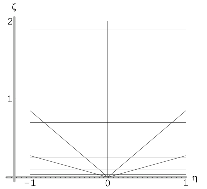
Figure 1: Translational Killing orbits in Poincaré upper half space. The dotted line, $\zeta=0$, marks the boundary of the hyperbolic space. The boundary is infinitely distant to any point in the interior ($\zeta>0$) of the space. The solid horizontal lines are equidistant orbits of $k_{1}$. The ray orbits correspond to $k_{2}$, and they too are equidistant. In both cases the distance between the orbits is unity if $\ell=1$. These orbits are also shown below in fig. 3.

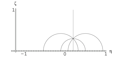
Figure 2: Geodesics in Poincaré upper half space. A sample of geodesics through a point at $\pi/4$ angular separation. Note that the angles in ${\mathbb{H}}^{2}$ coincide with the angles in ${\mathbb{E}}^{2}$ due to the conformal equivalence between the two spaces.

To understand fully the hyperbolic space geometry we must also know its geodesics. In contrast to the situation in flat space, the geodesics in hyperbolic space do not coincide with Killing orbits. Returning to the 2-dimensional upper half space picture, the geodesics are semicircles with centers on the line $\zeta=0$ (see fig. 2). The vertical lines are also geodesics and can be considered as a limiting case by moving the center of the circle along $\zeta=0$ to infinity. It should be kept in mind that the special appearance of the vertical geodesics is entirely due to the adopted representation. All geodesics are in fact equivalent due to complete isotropy and homogeneity of the hyperbolic space.

Our next task is to transform the above statements about the upper half space to the case of Poincaré disk. This can be achieved most transparently by using Möbius transformation to transform the upper half plane with complex coordinate $w=\eta+\mbox{i}\zeta$ into a unit disk. The required transformation is

$$w\rightarrow w^{\prime}:=y+\mbox{i}z=\frac{\mbox{i}w+1}{w+\mbox{i}}\ .$$ (17)

Relation between the disk coordinates, $(y,z)$, and the upper half space coordinates, $(\eta,\zeta)$, can also be written in the real form

$$y=\frac{2\eta}{\eta^{2}+\left(1+\zeta\right)^{2}}\ ,\qquad z=\frac{\eta^{2}+\zeta^{2}-1}{\eta^{2}+\left(1+\zeta\right)^{2}}\ .$$ (18)

This gives the 2-dimensional hyperbolic space in the Poincaré disk form

$$\,{}^{\scriptscriptstyle{(2)}}\negthinspace g_{\mbox{\tiny\rm{H}}}=\frac{4\ell^{2}}{\left(1-\tilde{\rho}^{2}\right)^{2}}\,\left({\rm d}y^{2}+{\rm d}z^{2}\right)\ ,$$ (19)

where $\tilde{\rho}^{2}=y^{2}+z^{2}$.

Let us start with the horizontal class of Killing orbits as given in fig. 1. These orbits appear as circles touching the north pole in the disk picture of fig. 3 (left panel). Clearly, the term horizontal does not apply to these orbits in the context of the disk representation. Instead they will be referred to as the north pole class of Killing orbits.

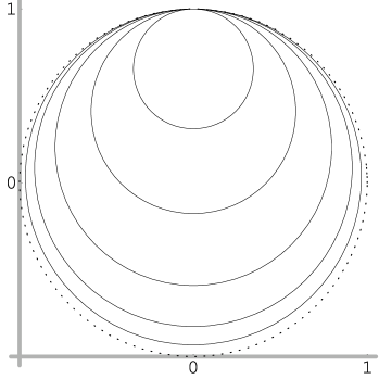
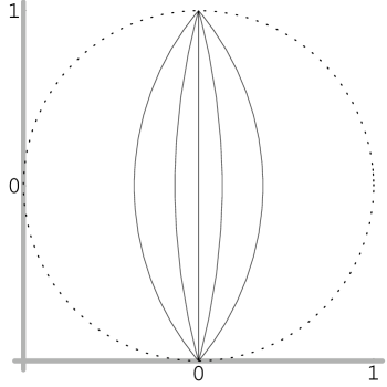
Figure 3: Two classes of Killing orbits are shown in the Poincaré disk, corresponding to the orbits plotted in fig. 1: The north pole class (left panel) is identical to the family of horizontal lines in fig. 1, while the meridional class (right panel) coincides with the family of ray orbits. The dotted circle represents the boundary of ${\mathbb{H}}^{2}$.

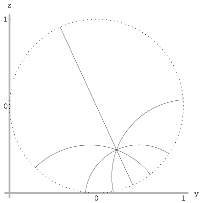
Figure 4: Geodesics in the Poincaré disk. A sample of geodesics at $\pi/4$ angular separation through the transformed reference point of fig. 2. As explained in text, however, these are not the same geodesics as those in that figure.

Next we consider, in more detail, the ray orbits from fig. 1. They too are circular in the disk but with the center of the circle lying outside the disk itself. The entire orbits are therefore represented by circular arcs inside the disk, and their appearances do not resemble rays anymore. We will refer to them as meridional Killing orbits (see fig. 3, right panel) because, in the 3-dimensional view, each such orbit gives rise to a surface of revolution which defines a meridional Killing cylinder.

Finally, we take a look at the geodesics in the disk picture. As in the upper half space, the geodesics are circles which meet the boundary at right angle, as illustrated in fig. 4. The straight lines going through the origin are geodesics that represent the limiting case when radius of the circle is infinite. The straight-line geodesics are in a one-to-one correspondence with those upper half space geodesics which pass through the point $w=i$ via eq. (17). A sample of geodesics is shown in fig. 4 (they have been constructed at $\pi/4$ angular separation). Note that the mapping (17) transforms the geodesics of fig. 2 to a different set of disk geodesics (also at $\pi/4$ angular separation).

4 Reissner-Nordström optical geometry embedded in a hyperbolic space

4.1 The embedding equations

When considering the embeddings in a hyperbolic space we need to find an embedding condition which replaces eq. (6) valid for flat space. For that purpose we introduce cylindrical coordinates $(\tilde{\chi},\phi,z)$ by

$$x=\tilde{\chi}\cos\phi\ ,\qquad y=\tilde{\chi}\sin\phi\ .$$ (20)

The Poincaré ball metric then takes the form

$$g_{\mbox{\tiny\rm{H}}}=\frac{4\ell^{2}}{\left(1-\tilde{\rho}^{2}\right)^{2}}\left({\rm d}\tilde{\chi}^{2}+\tilde{\chi}^{2}{\rm d}\phi^{2}+{\rm d}z^{2}\right)\,,$$ (21)

where $\tilde{\rho}^{2}=\tilde{\chi}^{2}+z^{2}$. The equatorial part of the optical geometry of a static spherically symmetric spacetime is given by the 2-metric (2). Comparing with the ball metric in cylindrical coordinates, eq. (21), we define the height function $h:=z$ and the cylindrical radius function $q:=\chi=\sqrt{x^{2}+y^{2}}$. This gives the embedding relations

$${\rm d}r_{\star}^{2}=\frac{4\ell^{2}}{\left(1-s^{2}\right)^{2}}\left({\rm d}q^{2}+{\rm d}h^{2}\right)\ ,\qquad\tilde{r}=\frac{2\ell q}{1-s^{2}}\ ,$$ (22)

where we have introduced $s^{2}:=q^{2}+h^{2}$. Just as for flat space embeddings there is an embedding condition which must be satisfied (this hyperbolic embedding condition will be discussed in section 4.2). When $\tilde{r}$ is a known function of $r_{\star}$, the equations (22) can be solved providing the embedding condition is satisfied. We have solved these equations numerically for some cases to be discussed below. Solving them analytically is not straightforward. However, it is possible to obtain further insight by first performing the embedding in the upper half space and then transforming to the ball picture. In fact, it turns out that the embedding relations can be rather easily solved analytically in that case.

We introduce cylindrical coordinates $(\chi,\phi,\zeta)$ for the upper half space by

$$\xi=\chi\cos\phi\ ,\qquad\eta=\chi\sin\phi\$$ (23)

(we do not distinguish the angle coordinates in different representations since we are only considering spaces with rotational symmetry). Writing the upper half space metric in cylindrical coordinates gives

$$g_{\mbox{\tiny\rm{H}}}=\ell^{2}\zeta^{-2}\left({\rm d}\chi^{2}+\chi^{2}{\rm d}\phi^{2}+{\rm d}\zeta^{2}\right)\ .$$ (24)

We define a height function $h(r)=\zeta$ and the cylindrical radius function $q(r)=\chi$ for the values of $\zeta$ and $\chi$ of the embedded surface. The two functions are determined by the embedding equations

$${\rm d}r_{\star}^{2}=\ell^{2}h^{-2}\left({\rm d}q^{2}+{\rm d}h^{2}\right)\ ,\quad\tilde{r}=\ell qh^{-1}\ .$$ (25)

These relations have a structure simpler than the corresponding equations for the ball embedding (22). To find the solution we first eliminate ${\rm d}{q}$ to obtain an equation which is quadratic in $(\ln h)^{\prime}$:

$$\left(\tilde{r}^{2}+\ell^{2}\right)\left(\ln h\right)^{\prime}{}^{2}+2\tilde{r}\tilde{r}^{\prime}\left(\ln h\right)^{\prime}+\tilde{r}^{\prime}{}^{2}-r^{\prime}_{\star}{}^{2}=0\ ,$$ (26)

where the prime stands for differentiation with respect to $r$. The solution is

$$(\ln h)^{\prime}=\frac{-\tilde{r}\tilde{r}^{\prime}+\sqrt{{\cal{}D}(r)}}{\tilde{r}^{2}+\ell^{2}}\ ,$$ (27)

where

$${\cal{}D}(r):=\tilde{r}^{2}r^{\prime}_{\star}{}^{2}+\ell^{2}\left(r^{\prime}_{\star}{}^{2}-\tilde{r}^{\prime}{}^{2}\right)\ ,$$ (28)

and the positive root has been chosen to ensure $h^{\prime}>0$. Integrating eq. (27) we obtain

$$h=\frac{1}{\sqrt{\tilde{r}^{2}(r)+\ell^{2}}}\exp\left\{\int{\frac{\sqrt{{\cal{}D}(r)}\,{\rm d}r}{\tilde{r}^{2}(r)+\ell^{2}}}\right\}\ .$$ (29)

In the Reissner-Nordström case we have

$${\cal{}D}(r)=\frac{r^{2}\left\{r^{6}+\ell^{2}\left[4Mr^{3}-3\left(3M^{2}+Q^{2}\right)r^{2}+12MQ^{2}r-4Q^{4}\right]\right\}}{\left(r^{2}-2Mr+Q^{2}\right)^{3}}\ .$$ (30)

Setting $x=r/M$, $\alpha=\ell/M$ and $\mu=Q/M$ we can now write the height function in the explicit form,

$$h(x)=K\,h_{\infty}f(x)\exp\left\{\int_{x_{\!\scriptscriptstyle\cal{H}}}^{x}g(u)\,{\rm d}u\right\}\ ,$$ (31)

where

$$f(x) = \frac{1}{\sqrt{\tilde{r}^{2}(r)+\ell^{2}}}=\sqrt{\frac{x^{2}-2x+\mu^{2}}{x^{4}+\alpha^{2}(x^{2}-2x+\mu^{2})}}\ ,$$

$$g(x) = \frac{\sqrt{{\cal{}D}(r)}}{\tilde{r}^{2}(r)+\ell^{2}}=\frac{x\sqrt{x^{6}+\alpha^{2}[4x^{3}-3(3+\mu^{2})x^{2}+12\mu^{2}x-4\mu^{4}]}}{[x^{4}+\alpha^{2}(x^{2}-2x+\mu^{2})]\sqrt{x^{2}-2x+\mu^{2}}}\ ,$$ (32)

and $x_{\!\scriptscriptstyle\cal{H}}=1+\sqrt{1-\mu^{2}}$ is the value of $x$ at the horizon. The expression (31) cannot be used as it stands to evaluate the height function. The reason is that the integral diverges in the limit $x\rightarrow\infty$ as will be discussed below. Moreover, for $Q=M$, the integral also diverges in the limit $x\rightarrow x_{\!\scriptscriptstyle\cal{H}}$. We now proceed to discuss the case $Q<M$, while the extremal case $Q=M$ can be dealt with along similar lines.

The value of the constant $K$ is assumed to be chosen such that $h_{\infty}$ is the asymptotic value of the height function in the limit $x\rightarrow\infty$. To see how this works, we must understand the behaviour of $h$ in that limit. We first note that $f(x)$ and $g(x)$ have the asymptotic forms

$$f(x)=\frac{1}{x}+{\cal O}\left(\frac{1}{x^{2}}\right)\ ,\qquad g(x)=\frac{1}{x}+\frac{1}{x^{2}}+{\cal O}\left(\frac{1}{x^{3}}\right)\ .$$ (33)

Defining

$${\cal{}S}(x):=xg(x)-1=\frac{1}{x}+{\cal O}\left(\frac{1}{x^{2}}\right)\ ,$$ (34)

we can then express $h$ in the form

$$h(x)=K\,h_{\infty}\,x_{\!\scriptscriptstyle\cal{H}}^{-1}xf(x)\exp\left\{\int_{x_{\!\scriptscriptstyle\cal{H}}}^{x}\frac{{\cal{}S}(u){\rm d}u}{u}\right\}\ .$$ (35)

Now, using the fact that $xf(x)\rightarrow 1$ as $x\rightarrow\infty$, we find that

$$K=x_{\!\scriptscriptstyle\cal{H}}\exp\left\{-\int_{x_{\!\scriptscriptstyle\cal{H}}}^{\infty}\frac{{\cal{}S}(u){\rm d}u}{u}\right\}\ .$$ (36)

It follows from the asymptotic form of ${\cal{}S}(x)$ that the integral in (36) is convergent and hence $K$ is a well-defined positive constant. The embedded surface is asymptotic to the plane $h=h_{\infty}$. The value of $h_{\infty}$ is arbitrary and reflects only a choice of scale which affects both $h$ and $q$ in the same way as seen from the embedding equations (25). From (9) and (25) we also obtain the cylindrical radius function:

$$q(x)=\frac{x^{2}h(x)}{\alpha\sqrt{x^{2}-2x+\mu^{2}}}\ .$$ (37)

The relations (31) and (37) together give the embedding of Reissner-Nordström optical geometry in the upper half space. The ball embedding functions can be readily computed from the upper half space embedding using the coordinate transformation (18):

$$\tilde{q}=\frac{2q}{q^{2}+(1+h)^{2}}\ ,\quad\tilde{h}=\frac{q^{2}+h^{2}-1}{q^{2}+(1+h)^{2}}\ .$$ (38)

4.2 The hyperbolic space embedding condition

A necessary condition for embedding is ${\cal{}D}(r)\geq 0$. This criterion can be expressed in the dimensionless form

$${\cal{}B}(r):=\frac{M^{2}}{\tilde{r}^{2}}\left[\left(\frac{{\rm d}\tilde{r}}{{\rm d}r_{\star}}\right)^{\!2}-1\right]\leq\frac{M^{2}}{\ell^{2}}\ .$$ (39)

In the limit of flat space embeddings, $\ell\rightarrow\infty$, this condition reduces to (6) as it should. It follows that the possibility of performing an embedding is governed by the quantity $\sup{\cal{}B}(r)$ where the supremum is taken over some desired radial range. The reasonable range in this context is $r>r_{\!\!\scriptscriptstyle\cal{H}}$ where $r_{\!\!\scriptscriptstyle\cal{H}}$ is the value of $r$ at the horizon. If $\sup{\cal{}B}(r)\leq 0$, then ${\mathbb{E}}^{3}$ can be used as embedding space. If, on the other hand, $0<\sup{\cal{}B}(r)<+\infty$ and if the radius of curvature satisfies the global embedding condition

$$\ell\leq M[\,\sup{\cal{}B}(r)]^{-1/2},$$ (40)

then hyperbolic spaces can be used. For the Reissner-Nordström solution we have

$${\cal{}B}(r)=M^{2}r^{-6}\left[-4Mr^{3}+3\left(3M^{2}+Q^{2}\right)r^{2}-12MQ^{2}r+4Q^{4}\right]\ .$$

If we restrict attention to the case $Q\leq M$, then this function attains its supremum at the (outer) horizon $r_{\!\!\scriptscriptstyle\cal{H}}=r_{+}=M+\sqrt{M^{2}-Q^{2}}$ with the value

$${\cal{}B}(r_{\!\!\scriptscriptstyle\cal{H}})=\sup_{r>r_{\!\!\scriptscriptstyle\cal{H}}}{\cal{}B}(r)=\frac{1-\mu^{2}}{\Bigl{(}1+\sqrt{1-\mu^{2}}\Bigr{)}^{4}}\ ,$$ (41)

where $\mu:=Q/M$. It follows that the global embedding condition (40) takes the form

$$\ell/M\leq 2+\frac{2-\mu^{2}}{\sqrt{1-\mu^{2}}}\ .$$ (42)

Thus for the Schwarzschild metric, the global embedding condition is $\ell/M\leq 4$. The right hand side of (42) increases monotonically with $\mu$ and obviously tends to infinity in the limit $\mu\rightarrow 1$. This implies that in the extreme Reissner-Nordström case, the optical geometry can in fact also be embedded in flat space.

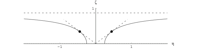
Figure 5: A vertical section of the embedded Schwarzschild geometry in the upper half space. As $r\rightarrow\infty$ the optical geometry is asymptotic to the Killing orbit represented by the dashed horizontal line. The neck at $r=3M$ is indicated by the black dots where the optical geometry touches the dashed Killing ray orbits.

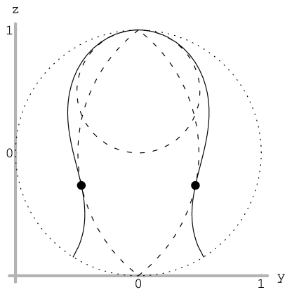
Figure 6: A vertical section of the embedded Schwarzschild geometry in the Poincaré ball. The dashed curves represent Killing orbits. The black dots mark the position of the neck at $r=3M$.

4.3 Physical properties of the embedding

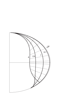
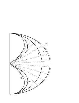
Figure 7: Azimuthal sections are plotted (thick solid curves) of the embedding surfaces in the Poincaré ball (denoted by the outer half-circle $\cal{}P$). Left panel: $Q=0$ (Schwarzschild black hole). Four cases of different ball curvature are shown; $\ell/M=0.1$, $1$, $2.4$, $4$. Right panel: $Q=M$ (maximally charged Reissner-Nordström black hole); $\ell/M=0.1$, $1$, $15$, $90$. The shape of the embedding curve resembles an arc if $\ell/M\rightarrow 0$ (infinite curvature), and it gets progressively more deformed when the curvature decreases. Dotted lines connect the points on the embedding curves with identical values of $r$. See the text for details.

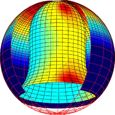
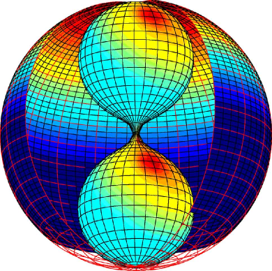
Figure 8: Poincaré ball embeddings. Three-dimensional view of the embedding diagrams is obtained by rotating the azimuthal section around $z$-axis of symmetry. Here we show two limiting cases corresponding to the graphs presented in fig. 7. Left panel: $Q/M=0$, $\ell/M=4$; right panel: $Q/M=1$, $\ell/M=90$.

We begin this section by discussing the behaviour of the embeddings in two limiting cases, $r\rightarrow\infty$ and $r\rightarrow r_{\!\!\scriptscriptstyle\cal{H}}$. Consider first the upper half space picture. It is clear from the analysis in section 4.1 that $h\rightarrow h_{\infty}$ as $r\rightarrow\infty$ where $h_{\infty}$ can be set to arbitrary positive number. Therefore the optical geometry defines an asymptote to the Killing plane $h=h_{\infty}$ for large $r$. This is illustrated in fig. 5 where a 2-dimensional section of the Schwarzschild optical geometry is shown. In the horizon limit, $h\rightarrow 0$ as can be seen from eq. (35) using the fact that $f(x_{\!\scriptscriptstyle\cal{H}})=0$. Thus the horizon is at infinity in the hyperbolic space, and the embedding is defined all the way down to (but not including) the horizon itself (see fig. 5 to illustrate this situation).

A particularly interesting aspect of the optical geometry of black holes and relativistic stars is the appearance of circular light orbits at constant radius. Such orbits correspond to necks and bulges in the optical geometry (see e.g. [4, 7]). The most well-known example of a neck is the one associated with the circular orbit at $r=3M$ in the Schwarzschild geometry. The existence of a neck implies that massless particles can be trapped in the region inside the neck. So, we turn to the manifestation of necks and bulges in the embedded surface. The condition for a neck (or a bulge) occurring at some radius $r_{0}$ is that the derivative $\tilde{r}^{\prime}(r_{0})=0$. From eq. (25) we see that this corresponds to $(q/h)^{\prime}=0$, which is precisely the condition that the surface is tangential to a ray passing through the origin. Clearly this is the same as being tangential to the orbits of the Killing vector field $k_{2}$. Since the embedded surface has rotational symmetry, it is actually tangential to a circular cone ruled by Killing orbits of the ray class in the upper half space representation. The neck at $r=3M$ is shown in fig. 5 together with two associated Killing rays. The appearence of necks can in fact be characterized in a simple way which is valid for any embedding with the rotational symmetry, thus including both the flat and the hyperbolic embeddings. Namely, the embedded surface has a neck precisely if it touches a surface of revolution that is ruled by Killing orbits parallel to the symmetry axis.

Reinterpreting these results in the Poincaré ball picture we find that the asymptotic optical geometry at infinity ($r\rightarrow\infty$) is tangential to a Killing 2-sphere defined by north pole Killing orbits. A 2-dimensional section of the Schwarzschild optical geometry embedded in the ball is illustrated in fig. 6. At the horizon, the optical geometry again stretches out to infinity, represented by the unit sphere with center at the origin, while at the $r=3M$ neck the optical geometry touches a meridional Killing cylinder.

Thus the main conclusions in this section are as follows: (i) asymptotic behaviour of the optical geometry for $r\rightarrow\infty$ is described by Killing orbits of the north pole class; (ii) necks and bulges occur when the optical geometry is tangential to the meridional Killing cylinder; and (iii) the horizon is at infinity of hyperbolic space.

Finally, the actual shapes of Poincaré ball embeddings of the Reissner-Nordström black hole are plotted in Figures 7–8. In each graph we consider two values of the charge for illustration: $Q=0$ (left panels) and $Q=M$ (right panels), respectively. First, fig. 7 shows $\tilde{\phi}={\rm{const}}$ sections of the embedding surface. The embedding shape touches the ball in its northern pole corresponding to spatial infinity ($r\rightarrow\infty$), and at the other point corresponding to the horizon ($r{\rightarrow}r_{\!\!\scriptscriptstyle\cal{H}}$). Notice that the latter point represents a circle on the embedding surface ($0\leq\phi<2\pi$) which gradually shrinks to the south pole of the ball as $Q{\rightarrow}M$. Thus, the embedding surface has no edge in the limiting case of $Q=M$, as shown in the right panel.

Each panel contains four lines of the same embedding curve which refer to different values of the curvature parameter $\ell/M$. We recall that the allowed range of $\ell/M$ is given by eq. (41): For $Q=0$, the minimum radius of curvature is $\ell=4M$, corresponding to the embedding curve crossing the ball perpendicularly at $r=2M$. In the strong curvature limit ($\ell/M\rightarrow 0$), the embedding surface asymptotically becomes spherical and hence approaches the ball. The situation is slightly more complicated for $Q=M$ and large curvature, when the neck develops on the embedding surface. A three-dimensional view of the embedding is obtained by rotating the embedding curve around symmetry axis; two such examples are plotted in fig. 8.

Notice that the right hand panels of figures 7 and 8, depicting the extremal case, are symmetric under reflection in a horizontal plane through the neck. This is not an accident: It is known [5] that the extremal Reissner-Nordström black hole admits a discrete conformal isometry that interchanges the region $M<r<2M$ with the region $r>2M$. For the optical geometry this transformation becomes a true isometry. Using the tortoise coordinate $r_{\star}$ it is simply a reflection $r_{\star}\rightarrow-r_{\star}$ through the neck, which is situated at $r_{\star}=0$.

5 Conclusions and future work

We have argued in this paper that the Poincaré ball embedding is a natural and useful tool to study global topological properties of spaces with negative curvature, for example the optical space of a black hole geometry. One particular subject that we plan to study using the Poincaré ball embeddings is the problem of topology of the event horizon in the optical space corresponding to the Reissner-Nordström solution. In the optical space, the event horizon is always located at infinity, corresponding to the surface of the Poincaré ball in the embedding. It is interesting to note that while for non-extremal ($Q<M$) black holes the region occupied by the horizon is finite (see fig. 8, left panel), in the case of an extremal black hole it shrinks to a single point (fig. 8, right panel). This is because the optical geometry of the extremal black hole is asymptotically flat at both ends.

References

References

- [1] Abramowicz M A 1993 Sci. Am. 268 74
- [2] Abramowicz M A, Andersson N, Bruni M, Ghosh P, Sonego S 1997 Class. Quantum Grav. 14, L189
- [3] Abramowicz M A, Carter B, Lasota J P 1988 Gen. Rel. Grav. 20 1173
- [4] Åminneborg S, Bengtsson I, Holst S, Peldán P 1996 Class. Quantum Grav. 13 2707
- [5] Couch W E, Torrence R J 1984 Gen. Rel. Grav. 16 789
- [6] Horowitz G T, 1998, in Wald R M (ed) Black Holes and Relativistic Stars (Chicago: University of Chicago Press), p 241
- [7] Karlovini M, Rosquist K, Samuelsson L 2001 Class. Quantum Grav. 18 817
- [8] Misner C W, Thorne K S, Wheeler J A 1973 Gravitation (San Francisco: Freeman)
- [9] Sonego S, Abramowicz M A 1998 J. Math. Phys. 39 3158
- [10] Sonego S, Almergren J, Abramowicz M A 2000 Phys. Rev. D 62 4010
- [11] Spivak M 1979 A Comprehensive Introduction to Differential Geometry (Houston: Publish and Perish, Inc.)
- [12] Thurston W P 1998 Class. Quantum Grav. 15 2545
- [13] Wald R M 1984 General Relativity (Chicago: University of Chicago Press)