Isolated Horizons in $2+1$ Gravity

Abstract

Using ideas employed in higher dimensional gravity, non-expanding, weakly isolated and isolated horizons are introduced and analyzed in 2+1 dimensions. While the basic definitions can be taken over directly from higher dimensions, their consequences are somewhat different because of the peculiarities associated with 2+1 dimensions. Nonetheless, as in higher dimensions, we are able to: i) analyze the horizon geometry in detail; ii) introduce the notions of mass, charge and angular momentum of isolated horizons using geometric methods; and, iii) generalize the zeroth and the first laws of black hole mechanics. The Hamiltonian methods also provide, for the first time, expressions of total angular momentum and mass of charged, rotating black holes and their relation to the analogous quantities defined at the horizon. We also construct the analog of the Newman-Penrose framework in 2+1 dimensions which should be useful in a wide variety of problems in 2+1 dimensional gravity.

Center for Gravitational Physics and Geometry, Department of Physics, The Pennsylvania State University, University Park, PA 16802, USA

ashtekar@gravity.phys.psu.edu

Perimeter Institute for Theoretical Physics, 35 King Street North, Waterloo, Ontario N2J 2W9, Canada

odreyer@perimeterinstitute.ca

Center for Gravitational Physics and Geometry, Department of Physics, The Pennsylvania State University, University Park, PA 16802, USA

jacek@phys.psu.edu

1 Introduction

The zeroth and first laws of black hole mechanics apply to equilibrium situations and small departures therefrom. In standard formulations of these laws, black holes in equilibrium are represented by stationary space-times with regular event horizons (see, e.g., [1, 2]). While this idealization is a natural starting point, from a physical perspective it seems quite restrictive. (See [3, 4] for a detailed discussion.) To overcome this limitation, a new model for a black hole in equilibrium was recently introduced for 3+1 (and higher) dimensional gravity [3, 4, 5, 6]. The generalization is two-fold. First, one replaces the notion of an event horizon with that of an isolated horizon. While the former are defined only retroactively using the fully evolved space-time geometry, the latter are defined quasi-locally by suitably constraining the geometry of the horizon surface itself. Second, one drops the requirement that the space-time be stationary and asks only that the horizon be isolated. That is, the requirement that the black hole be in equilibrium is incorporated by demanding only that no matter or radiation fall through the horizon although the exterior space-time region may well admit radiation. Consequently, the generalization in the class of allowed space-times is enormous. In particular, space-times admitting isolated horizons need not possess any Killing vector field; although event horizons of stationary black holes are isolated horizons, they are a very special case. A recent series of papers [4, 5, 6, 7] has generalized the laws of black hole mechanics to this broader context. The notion of isolated horizons has proved to be useful also in other contexts in 3+1 dimensions, ranging from numerical relativity to background independent quantum gravity: i) it plays a key role in an ongoing program for extracting physics from numerical simulations of black hole mergers [8, 9, 10, 11]; ii) it has led to the introduction [5, 12, 13] of a physical model of hairy black holes, systematizing a large body of results on properties of these black holes which has accumulated from a mixture of analytical and numerical investigations; and, iii) it serves as a point of departure for statistical mechanical entropy calculations in which all black holes (extremal or not) and cosmological horizons are incorporated in a single stroke [3, 14, 15].

In recent years, 2+1-dimensional stationary black holes have drawn a great deal of attention as simplified models for analyzing conceptual issues surrounding black hole thermodynamics (see, e.g., [2]). It is therefore natural to ask if the isolated horizon framework can be constructed and used to extend the standard 2+1-dimensional treatments. The purpose of this paper is to provide such a framework, analyze the resulting horizon geometry in detail and use it to generalize the zeroth and first laws of black hole mechanics.

In Section 2, we introduce the definitions of non-expanding and weakly isolated horizons and derive their main consequences, including the generalized zeroth law. While the basic definitions are the same as in higher dimensions, some of their consequences are different because of special features of the 3-dimensional Riemannian geometry [16]. In particular, the Weyl tensor, which plays an important role in higher dimensions, now vanishes identically. Similarly, since in 2+1 dimensions black holes exist only if the cosmological constant is non-zero, there is now an inherent length scale in the problem. However, the spirit of the analysis is the same as in higher dimensions: We extract, from the notion of Killing horizons, the minimal structure that is needed to generalize the laws of black hole mechanics. As in 3+1 dimensions, some of the structure becomes more transparent in terms of null-triads. Therefore, in Appendix A we construct the 2+1-dimensional analog of the Newman-Penrose framework [17] and use it to elucidate the meaning and consequences of our horizon boundary conditions.

In Section 3 we introduce the action principle, and in Section 4, the covariant phase space and the associated Hamiltonian framework. While the overall procedure is the same as in higher dimensions [5, 6], there is a significant technical complication in the choice of boundary conditions at infinity. In particular, while the electromagnetic potential falls off as $1/r^{n}$ in $n+2$ spatial dimensions for $n>0$, one must now allow it to blow up logarithmically. Since the treatment of these boundary conditions is perhaps the most difficult technical part of our analysis, they are spelled out in detail separately in Appendix B. The end result is that there do exist boundary conditions which suffice to make the action principle, the symplectic structure and the Hamiltonians well-defined. Using these structures, we establish the generalized first law. As in higher dimensions, it arises as a consistency condition for the evolution to be generated by a Hamiltonian; there is thus an infinite family of first laws, one for each time-like vector field in space-time, the evolution along which is Hamiltonian.

In Section 5, we consider the issue of introducing a canonical notion of horizon energy which can be interpreted as horizon mass. In the Hamiltonian framework, this problem reduces to that of selecting (for each point in the phase space) a preferred time-evolution vector field at the horizon. One expects this choice to vary from one point in the phase space to another; in the non-rotating case, one would expect the preferred vector field to point along the null normal to the horizon, while in the rotating case, one would expect it to have a non-zero component also along the space-like, rotational direction at the horizon. As in 3+1 dimensions, we resolve this problem by making use of known stationary solutions [18, 19, 20].

Sections 3-5 focus on the infinite dimensional space of histories and the phase space in presence of weakly isolated horizons. In Section 6, by contrast, we consider individual space-times and analyze the geometrical structures and their interplay with field equations at the horizon. Specifically, we first show that non expanding horizons admit a natural derivative operator ${\cal D}$ and study the geometrical information it encodes, beyond the natural degenerate metric, and then use field equations to isolate the freely specifiable parts of ${\cal D}$ on weakly isolated horizons. As in higher dimensions [5] we introduce the notion of isolated horizons using the derivative operator ${\cal D}$. In contrast to higher dimensions, every non-expanding horizon can be equipped with an isolated horizon structure simply by selecting an appropriate null normal and, generically, this can be achieved in a unique fashion. Readers who are primarily interested in the notions of mass and angular momentum and black hole mechanics can skip this section. Reciprocally, readers who are primarily interested in the horizon geometry and field equations can go directly to Section 6 after Section 2 without loss of continuity. Section 7 summarizes the main results and points out a subtlety in the definition of mass which arises again because in 2+1 dimensions, the electromagnetic potential must be allowed to diverge logarithmically at infinity.

Throughout this paper, we will set $8\pi G=c=1$. Since Newton’s constant has dimensions of inverse mass in 2+1 dimensions, now mass and charge are dimensionless while angular momentum has dimensions of length. As a general rule, arguments and proofs which are parallel to those in higher dimensions [5, 6, 10] are only sketched and differences are emphasized.

2 Definitions and geometrical structures

In this Section we will define weakly isolated horizons and analyze their geometric properties. It is convenient to proceed in two steps since certain preliminary results are needed to state the final definition.

Let ${\mathcal{M}}$ be a three dimensional manifold with metric tensor $g_{ab}$ of signature $(-\,+\,+)$. For simplicity, we will assume that all manifolds and fields are smooth. Let $\Delta$ be a null hypersurface in $({\mathcal{M}},g_{ab})$. A future directed null normal to $\Delta$ will be denoted by $\ell$. The expansion $\theta_{(\ell)}$ of $\ell$ is defined by $\theta_{(\ell)}\widehat{=}m^{a}m^{b}\nabla_{a}\ell_{b}$, where $\nabla$ is the derivative operator on $({\mathcal{M}},g_{ab})$ and $m^{a}$ is any unit, space-like vector field tangent to $\Delta$. It is easy to check that the expansion is insensitive to the choice of $m^{a}$. However, as the notation suggests, it does depend on the choice of the null normal $\ell$; if $\ell^{\prime}\widehat{=}f\ell$, then $\theta_{(\ell^{\prime})}\widehat{=}f\theta_{(\ell)}$.

2.1 Non-expanding horizons

Definition 1: A $2$-dimensional sub-manifold $\Delta$ of a space-time $({\mathcal{M}},g_{ab})$ is said to be a non-expanding horizon if it satisfies the following conditions:

(i) $\Delta$ is topologically $S^{1}\times{\mbox{\rm$\mbox{I}\!\mbox{R}$}}$ and null;

(ii) The expansion $\theta_{(\ell)}$ of $\ell$ vanishes on $\Delta$ for any null normal $\ell$;

(iii) All equations of motion hold at $\Delta$ and the stress-energy tensor $T_{ab}$ of matter fields at $\Delta$ is such that $-T^{a}_{\ b}\ell^{b}$ is future directed and causal for any future directed null normal $\ell$.

Note that if conditions (ii) and (iii) hold for one null normal $\ell$ they hold for all.

The role of these conditions is as follows. The first condition just ensures that the cross-sections of $\Delta$ are compact which will in turn ensure that various integrals —defining, e.g., the symplectic structure and various Hamiltonians— over these cross-sections are well-defined. The second condition is the crucial one. It directly implies that all horizon cross-sections have the same length, which, following the terminology in the literature [2] we will call the ‘horizon area’ and denote by $a_{\Delta}$. It will also be convenient to introduce the notion of the horizon radius $R_{\Delta}$, defined by $a_{\Delta}=2\pi R_{\Delta}$. Finally, as we will see below, condition (ii) also implies that there is no flux of matter-energy across the horizon and thus captures the intuitive notion that the black hole is isolated. The last condition, (iii), is analogous to the dynamical conditions one imposes at spatial infinity. While at infinity one requires that the metric (and other fields) approach a specific solution to the field equations (namely, ‘the classical vacuum’), at the horizon one only asks that the field equations be satisfied. The energy condition involved is very weak; it follows from the much stronger dominant energy condition normally imposed. All these conditions are satisfied on any Killing horizon (with a $S^{1}$ cross-section) if gravity is coupled to physically reasonable matter (including perfect fluids, Klein-Gordon fields, Maxwell fields possibly with dilatonic coupling and Yang-Mills fields).

We will now present three examples of non-expanding horizons:

Example 1: The paradigmatic example of a non-expanding horizon in 2+1 dimensions is provided by the BTZ black holes[18]. We begin by showing that the horizons of these space-times trivially satisfy our Definition 1.

In Eddington-Finkelstein-like coordinates, the space-time metrics of these black holes are given by

$$ds^{2}=-(N)^{2}dv^{2}+2dvdr+r^{2}\left(d\phi+N^{\phi}dv\right)^{2},$$ (2.1)

where

$$N=\left(f(r)+\frac{J^{2}}{4\pi^{2}r^{2}}\right)^{1/2}\mbox{ and\ }N^{\phi}=-\frac{J}{2\pi r^{2}},$$ (2.2)

and

$$f(r)=-\frac{M}{\pi}+\frac{r^{2}}{l^{2}},$$ (2.3)

the length $l$ being related to the cosmological constant $\Lambda$ through

$$\Lambda=-\frac{1}{l^{2}}.$$ (2.4)

Thus, for any value $\Lambda$ of the cosmological constant, there is a 2-parameter family of BTZ metrics, labeled by $M$ and $J$. The metric coefficient $N$ vanishes at $r=r_{\pm}$, where

$$r^{2}_{\pm}=\frac{Ml^{2}}{2\pi}\left\{1\pm\left[1-\left(\frac{J}{Ml}\right)^{2}\right]^{1/2}\right\}\,.$$ (2.5)

The 2-surface $r=r_{+}$ is the horizon of interest to us. Sometimes it is convenient to have the mass $M$ and the angular momentum $J$ expressed in terms of $r_{+}$ and $r_{-}$:

$$M=\pi\frac{r_{+}^{2}+r_{-}^{2}}{l^{2}}\ \ \ \ \ J=\frac{2\pi r_{+}r_{-}}{l}\,.$$ (2.6)

The surface $r=r_{+}$ is null with normal

$$\ell=\partial_{v}-N^{\phi}(r_{+})\partial_{\phi}.$$ (2.7)

Since it is coordinatized by $v,\phi$, it has the required topology, $S^{1}\times{\mbox{\rm$\mbox{I}\!\mbox{R}$}}$. Since $\ell$ is a restriction to the horizon of a space-time Killing field $\partial_{v}-N^{\phi}(r_{+})\partial_{\phi}$ it follows that $\theta_{(\ell)}$ vanishes. Finally, the third condition in the definition is trivially satisfied because BTZ metrics are vacuum solutions to Einstein’s equation.

Example 2: The first two conditions in our definition are satisfied by the more general class of metrics (2.1), without the restriction (2.3) on the form of the function $f(r)$. If the function $f(r)$ is chosen to satisfy the weak condition $(\partial_{r}f)\mid_{r=r_{+}}\leq(r_{+}/l^{2})$, the third condition in the definition is also satisfied. Thus, we have a very large class of generalized BTZ metrics which admit a non-expanding horizon. This class includes, in particular, the metrics introduced in [19].

Example 3: Our final example is the charged, rotating black hole solution first discovered by Clément [20]. (It was later independently found by Martinez, Teitelboim and Zanelli (MTZ) [21], who also analyzed its physical properties.) It is again a stationary axi-symmetric solution and is expressed in terms of three parameters, $\bar{r}_{0},\omega,Q$. As shown in section 5.2, they can be traded for mass $M$, angular momentum $J$ and charge $Q$. However, as in higher dimensional dilatonic black holes, the dependence of $M$ and $J$ on the parameters appearing explicitly in the solution is quite complicated (see Section 5). Furthermore, in this case, the electro-magnetic fields and the metric coefficients diverge (logarithmically) at infinity. Hence the very meaning of mass and angular momentum is not a priori transparent. Finally, if one simply sets $Q=0$, one obtains the BTZ metric with $M=0$ and $J=0$; to obtain the non-trivial solutions in the BTZ family, a more subtle limit has to be taken.

Clément gave the metric in the form:

$${\rm d}s^{2}=-N^{2}{\rm d}t^{2}+K^{2}({\rm d}\phi+N^{\phi}{\rm d}t)^{2}+\frac{r^{2}}{K^{2}}\frac{{\rm d}r^{2}}{N^{2}},$$ (2.8)

where the functions $N,N^{\phi}$ and $K$ are given by

$$N^{2} = \frac{r^{2}}{K^{2}}\left(\frac{r^{2}}{l^{2}}-\frac{\bar{l}^{2}}{2\pi l^{2}}Q^{2}\ln(r/\bar{r}_{0})\right),$$ (2.9)

$$N^{\phi} = -\frac{\omega}{2\pi K^{2}}Q^{2}\ln(r/\bar{r}_{0}),$$ (2.10)

$$K^{2} = r^{2}+\frac{1}{2\pi}\omega^{2}Q^{2}\ln(r/\bar{r}_{0}),$$ (2.11)

$$\bar{l}^{2} = l^{2}-\omega^{2}$$ (2.12)

The Maxwell field is given by:

$${\mathbf{F}}=\frac{Q}{r}{\rm d}r\wedge({\rm d}t-\omega{\rm d}\phi).$$ (2.13)

In the Eddington-Finkelstein-like coordinates the metric becomes

$${\rm d}s^{2}=-N^{2}{\rm d}v^{2}+\frac{2r}{K}{\rm d}v{\rm d}r+K^{2}\left({\rm d}\phi+N^{\phi}{\rm d}v\right)^{2}.$$ (2.14)

(As is usual in the passage to the Eddington-Finkelstein type coordinates in the stationary context, the angle $\phi$ in (2.14) is not the same as the one in (2.8). In the analysis of the horizon structure, we will use (2.14).) It is straightforward to check that the 2-surfaces $N=0$, co-ordinatized by $v,\phi$, are non-expanding horizons.

Although the conditions imposed in Definition 1 seem rather weak, they have a number of interesting consequences. To explore them it is often convenient to introduce, as in the Newman-Penrose framework, a triad consisting of vectors $\ell^{a},n^{a},$ and $m^{a}$ in the neighborhood of the horizon $\Delta$. The vectors $\ell^{a}$ and $n^{a}$ are null and $m^{a}$, space-like. We choose $\ell^{a}$ to be a future pointing null normal of the horizon and then normalize $n^{a}$ by requiring $\ell^{a}n_{a}\widehat{=}-1$ and $m^{a}$ by requiring $m^{a}m_{a}=1$. All other contractions vanish. (Thus, in contrast to the 3+1 dimensional NP framework, $m^{a}$ is now real and space-like rather than complex and null.) On the horizon we further require $m^{a}$ to be tangential to the horizon. Given such a triad, we can introduce NP-like coefficients as in 3+1 dimensions. Appendix A gives the corresponding definitions and a summary of important relations for these coefficients. It is often convenient to use the triad so that the pull-back to $\Delta$ of the 1-form $n$ is orthogonal to $S^{1}$ cross-sections of $\Delta$, i.e., ${\mathchoice{\vtop{\halign{#\cr$\textstyle{dn}$\crcr\kern-1.72218pt\nointerlineskip\cr{\tiny\leftarrowfill}\crcr}}}{\vtop{\halign{#\cr$\textstyle{dn}$\crcr\kern-1.72218pt\nointerlineskip\cr{\tiny\leftarrowfill}\crcr}}}{\vtop{\halign{#\cr\hfil$\scriptstyle{dn}$\hfil\crcr\kern 1.72218pt\nointerlineskip\cr{\tiny\leftarrowfill}\crcr}}}{\vtop{\halign{#\cr\hfil$\scriptstyle{dn}$\hfil\crcr\kern 1.72218pt\nointerlineskip\cr{\tiny\leftarrowfill}\crcr}}}}\vphantom{dn}\widehat{=}0$ (so that, in the NP-like framework of Appendix C, $\alpha\widehat{=}\pi$). We will explicitly specify when this restriction is made.

We will conclude this subsection with a brief discussion of geometric structures available on non-expanding horizons.

(a) Intrinsic metric of $\Delta$: Denote by $q_{ab}$ the pull-back of the space-time metric $g_{ab}$ to $\Delta$; $q_{ab}\widehat{=}g_{{\mathchoice{\vtop{\halign{#\cr$\textstyle{ab}$\crcr\kern-1.20552pt\nointerlineskip\cr{\tiny\leftarrowfill}\crcr}}}{\vtop{\halign{#\cr$\textstyle{ab}$\crcr\kern-1.20552pt\nointerlineskip\cr{\tiny\leftarrowfill}\crcr}}}{\vtop{\halign{#\cr\hfil$\scriptstyle{ab}$\hfil\crcr\kern 1.20552pt\nointerlineskip\cr{\tiny\leftarrowfill}\crcr}}}{\vtop{\halign{#\cr\hfil$\scriptstyle{ab}$\hfil\crcr\kern 1.20552pt\nointerlineskip\cr{\tiny\leftarrowfill}\crcr}}}}\vphantom{ab}}$. Since $\Delta$ is a 2-dimensional, null sub-manifold of $({\mathcal{M}},g_{ab})$, and $\ell$ a null-normal to it, it follows that

$$q_{ab}\ell^{b}\widehat{=}0;\quad\quad q_{ab}\widehat{=}\underline{m}_{a}\underline{m}_{b}$$ (2.15)

for a unique 1-form $\underline{m}_{a}$, defined intrinsically on $\Delta$. Furthermore, as the explicit calculation of spin coefficients in Appendix A shows, $d\underline{m}\widehat{=}0$. We will choose our NP triad such that $m_{{\mathchoice{\vtop{\halign{#\cr$\textstyle{a}$\crcr\kern-1.20552pt\nointerlineskip\cr{\tiny\leftarrowfill}\crcr}}}{\vtop{\halign{#\cr$\textstyle{a}$\crcr\kern-1.20552pt\nointerlineskip\cr{\tiny\leftarrowfill}\crcr}}}{\vtop{\halign{#\cr\hfil$\scriptstyle{a}$\hfil\crcr\kern 1.20552pt\nointerlineskip\cr{\tiny\leftarrowfill}\crcr}}}{\vtop{\halign{#\cr\hfil$\scriptstyle{a}$\hfil\crcr\kern 1.20552pt\nointerlineskip\cr{\tiny\leftarrowfill}\crcr}}}}\vphantom{a}}=\underline{m}_{a}$.

(b) Properties of $\ell$: Since $\ell^{a}$ is a null normal to $\Delta$, it is automatically twist-free and geodesic. We will denote the acceleration of $\ell^{a}$ by $\kappa_{(\ell)}$

$$\ell^{a}\nabla\!_{a}\ell^{b}\widehat{=}\kappa_{(\ell)}\ell^{b}\,.$$ (2.16)

Note that the acceleration is a property not of the horizon $\Delta$ itself, but of a specific null normal to it: if we replace $\ell$ by $\ell^{\prime}\widehat{=}f\ell$, then the acceleration changes via

$$\kappa_{(\ell^{\prime})}\widehat{=}f\kappa_{(\ell)}+{\cal L}_{\ell}f.$$ (2.17)

(In the NP-type notation of Appendix A, $\kappa_{(\ell)}$ is denoted by $\epsilon$.)

(c) A natural connection 1-form on $(\Delta,\ell)$: Since the expansion $\theta_{(\ell)}$ (or, in the framework of Appendix A, the NP-type coefficient $\rho$) vanishes, and since in 2+1 dimensions there is no analog of the 3+1 dimensional shear, we conclude that given any vector field $X^{a}$ tangential to $\Delta$, we have:

$$X^{a}\nabla_{a}\ell^{b}\widehat{=}X^{a}\omega_{a}\,\ell^{b}$$

for some ($\ell$-dependent) 1-form $\omega_{a}$ on $\Delta$. In particular, we have $\kappa_{(\ell)}=\ell^{a}\omega_{a}$. Thus, there exists a one-form $\omega_{a}$ intrinsic to $\Delta$ such that

$$\nabla\!_{\!{\mathchoice{\vtop{\halign{#\cr$\textstyle{a}$\crcr\kern-1.20552pt\nointerlineskip\cr{\tiny\leftarrowfill}\crcr}}}{\vtop{\halign{#\cr$\textstyle{a}$\crcr\kern-1.20552pt\nointerlineskip\cr{\tiny\leftarrowfill}\crcr}}}{\vtop{\halign{#\cr\hfil$\scriptstyle{a}$\hfil\crcr\kern 1.20552pt\nointerlineskip\cr{\tiny\leftarrowfill}\crcr}}}{\vtop{\halign{#\cr\hfil$\scriptstyle{a}$\hfil\crcr\kern 1.20552pt\nointerlineskip\cr{\tiny\leftarrowfill}\crcr}}}}\vphantom{a}}\ell^{b}\widehat{=}\omega_{a}\ell^{b}\,.$$ (2.18)

$\omega_{a}$ will play an important role in this paper. (In the NP-type framework of Appendix A, $\omega$ can be expressed in terms of spin coefficients: $\omega_{a}=\alpha\underline{m}_{a}-\epsilon n_{a}\equiv\alpha\underline{m}_{a}-\kappa_{(\ell)}n_{a}\,$.) Under the rescaling $\ell\rightarrow f\ell$, the 1-form $\omega$ transforms as a connection:

$${}\omega_{a}\rightarrow\omega_{a}+\nabla_{\!{\mathchoice{\vtop{\halign{#\cr$\textstyle{a}$\crcr\kern-1.20552pt\nointerlineskip\cr{\tiny\leftarrowfill}\crcr}}}{\vtop{\halign{#\cr$\textstyle{a}$\crcr\kern-1.20552pt\nointerlineskip\cr{\tiny\leftarrowfill}\crcr}}}{\vtop{\halign{#\cr\hfil$\scriptstyle{a}$\hfil\crcr\kern 1.20552pt\nointerlineskip\cr{\tiny\leftarrowfill}\crcr}}}{\vtop{\halign{#\cr\hfil$\scriptstyle{a}$\hfil\crcr\kern 1.20552pt\nointerlineskip\cr{\tiny\leftarrowfill}\crcr}}}}\vphantom{a}}\ln f.$$ (2.19)

A particular consequence of (2.18) is:

$${{\cal L}}_{\ell}\,q_{ab}\widehat{=}2{\mathchoice{\vtop{\halign{#\cr$\textstyle{\nabla\!_{a}\ell_{b}}$\crcr\kern-1.72218pt\nointerlineskip\cr{\tiny\leftarrowfill}\crcr}}}{\vtop{\halign{#\cr$\textstyle{\nabla\!_{a}\ell_{b}}$\crcr\kern-1.72218pt\nointerlineskip\cr{\tiny\leftarrowfill}\crcr}}}{\vtop{\halign{#\cr\hfil$\scriptstyle{\nabla\!_{a}\ell_{b}}$\hfil\crcr\kern 1.72218pt\nointerlineskip\cr{\tiny\leftarrowfill}\crcr}}}{\vtop{\halign{#\cr\hfil$\scriptstyle{\nabla\!_{a}\ell_{b}}$\hfil\crcr\kern 1.72218pt\nointerlineskip\cr{\tiny\leftarrowfill}\crcr}}}}\vphantom{\nabla\!_{a}\ell_{b}}\widehat{=}0\,;$$

every null normal $\ell$ to $\Delta$ is a ‘Killing field’ of the degenerate metric on $\Delta$. Thus, our key condition in the Definition —that $\ell$ be expansion-free— implies that non-expanding horizons are Killing horizons of the intrinsic geometry to ‘first order’.

Example 1: What is the expression of $\omega_{a}$ in the case of the BTZ black hole? On the horizon, let us choose the triad vector $m^{a}$ as $m\widehat{=}(1/r_{+})\partial_{\phi}$. Then, a direct calculation yields:

$$\omega_{a}=N^{\phi}m_{a}-\kappa_{(\ell)}n_{a}$$ (2.20)

where the acceleration $\kappa_{(\ell)}$ is given by

$$\kappa_{(\ell)}=\frac{r_{+}}{l^{2}}-r(N^{\phi})^{2}.$$ (2.21)

(See the discussion of this example in appendix A.) As in higher dimensions [4, 6], the angular momentum information is contained in the spatial component of $\omega$.

(d)Conditions on the Ricci tensor: As in higher dimensions [5], we can use the Raychaudhuri equation to obtain conditions satisfied by the 3-dimensional Ricci tensor at the horizon. Thus, by calculating ${\cal L}_{\ell}\,\,\theta_{(\ell)}$ for a general null congruence $\ell$ in terms of the derivatives of $\ell$ and the Ricci tensor and applying it to any normal of a non-expanding horizon, we obtain:

$$R_{ab}\ell^{a}\ell^{b}\widehat{=}0.$$ (2.22)

(For a derivation in the NP-type framework, see equation (A.33) in appendix A.) Next, let us use the energy condition required in the Definition: $P^{a}:\widehat{=}-T^{a}_{b}\ell^{b}$ is future pointing, and time-like or null on $\Delta$. Using the field equations

$$R_{ab}-\frac{1}{2}R\,g_{ab}+g_{ab}\Lambda=T_{ab}$$ (2.23)

and (2.22), we obtain $P_{a}\ell^{a}\widehat{=}0$, whence, at the horizon, $P^{a}$ is of the form $P^{a}\widehat{=}f\ell^{a}+gm^{a}$. The energy condition now implies $g\widehat{=}0$, i.e., the component $T^{a}_{\ b}\ell^{b}$ is proportional to $\ell^{a}$. The field equations then imply:

$$R_{ab}\ell^{a}m^{b}\widehat{=}0.$$ (2.24)

This constraint on the Ricci curvature has an important consequence. Using the expression of the 3-dimensional Riemann tensor in terms of the Ricci tensor in the equality $2\nabla_{[a}\nabla_{b]}\ell^{d}\widehat{=}R_{abc}{}^{d}\ell^{c}$, and (2.18), it is straightforward to express $d\omega$ in terms of $R_{ab}\ell^{a}m^{b}$. (2.24) now implies that $\omega$ is exact:

$$d\omega\widehat{=}0.$$ (2.25)

(In the NP-type framework of Appendix A, $R_{ab}m^{a}\ell^{b}$ can be expressed in terms of spin-coefficients as $R_{ab}m^{a}\ell^{b}\widehat{=}{\cal L}_{\ell}\,\pi-{\cal L}_{m}\,\kappa_{NP}$ and $d\omega\,\widehat{=}$ $({\cal L}_{\ell}\,\pi-{\cal L}_{m}\,\kappa_{NP})\,m\wedge n$, whence (2.24) implies that $\omega$ is exact.) By contrast, in 3+1 dimensions, $d\omega$ is essentially determined by the imaginary part of the Weyl tensor component $\Psi_{2}$, which encodes the angular momentum information [6]. We will see that angular momentum information continues to reside in $\omega$; it is just that, since the Weyl tensor vanishes identically in 3 dimensions, we can no longer further simplify that expression and rewrite it in terms of the $\Psi_{2}$.

(e) Projective space: Since $\ell$ Lie-drags the intrinsic metric $q_{ab}$ of $\Delta$, it is natural to pass to the space $\hat{\Delta}$ of orbits of $\ell$. We will conclude the discussion of non-expanding horizons with a discussion of $\hat{\Delta}$.

It follows from our topological restriction in Definition 1 that $\hat{\Delta}$ has the topology of $S^{1}$. Denote by $\hat{\Pi}$ the canonical projection map from $\Delta$ to $\hat{\Delta}$. Then, since $q_{ab}\ell^{b}\widehat{=}0$ and ${\cal L}_{\ell}\,q_{ab}\widehat{=}0$, it follows that there exists a metric $\hat{q}_{ab}$ on $\hat{\Delta}$ such that ${q}_{ab}\widehat{=}\hat{\Pi}_{\star}\hat{q}_{ab}$. The metric $\hat{q}_{ab}$ on $\hat{\Delta}$ can be uniquely expressed as $\hat{q}_{ab}=\hat{m}_{a}\hat{m}_{b}$ and $\underline{m}_{a}=\hat{\Pi}_{\star}\hat{m}_{a}$.

2.2 Weakly isolated horizons

Although non-expanding horizons already have a rather rich structure, the notion is not sufficiently strong to be directly useful to black hole mechanics. In particular, as we have seen, there is a freedom to rescale the null normal via $\ell^{a}\rightarrow{\ell^{\prime}}^{a}=f\ell^{a}$ for any positive function $f$ on $\Delta$ under which the acceleration of $\ell$ transforms via $\kappa_{(\ell^{\prime})}=f\kappa_{(\ell)}+{\cal L}_{\ell}\,f$. Because of this rescaling freedom, ${\kappa_{(\ell)}\,}$ will not be constant for a generic choice of $\ell$. Thus, on a general non expanding horizon, we can not hope to establish the zeroth law. In this sub-section, we will introduce a stronger definition by adding the minimal requirements needed for a natural generalization of black hole mechanics.

Let us begin by introducing an equivalence relation on the space of null normals to a non-expanding horizon $\Delta$. The transformation property (2.19) of $\omega_{a}$ under rescalings of $\ell^{a}$ shows that $\omega_{a}$ remains unaltered if and only if $\ell^{a}$ is rescaled by a constant. Therefore it is natural to regard two null normals as equivalent if they differ only by a (positive) constant rescaling. We will denote each of these equivalence classes by $[\ell]$. In what follows we will be interested in non-expanding horizons $\Delta$, equipped with such an equivalence class $[\ell]$ of null normals.

Definition 2: A weakly isolated horizon $(\Delta,[\ell])$ consists of a non-expanding horizon $\Delta$, equipped with an equivalence class $[\ell]$ of null normals satisfying

$${\cal L}_{\ell}\omega\widehat{=}0\,\,\,{\hbox{\rm for all}}\,\,\ell\in[\ell].$$ (2.26)

As pointed out above, if this last equation holds for one $\ell$, it holds for all $\ell$ in $[\ell]$. Condition (2.26) strengthens the notion that $\Delta$ has ‘reached equilibrium’: where as the intrinsic metric $q_{ab}$ is ‘time-independent’ on any non-expanding horizon, on a weakly isolated horizon, the connection 1-form $\omega$ is also ‘time-independent’. Since $\ell^{a}$ is normal to $\Delta$, one can regard $K_{a}{}^{b}:=\nabla_{\mathchoice{\vtop{\halign{#\cr$\textstyle{a}$\crcr\kern-1.20552pt\nointerlineskip\cr{\tiny\leftarrowfill}\crcr}}}{\vtop{\halign{#\cr$\textstyle{a}$\crcr\kern-1.20552pt\nointerlineskip\cr{\tiny\leftarrowfill}\crcr}}}{\vtop{\halign{#\cr\hfil$\scriptstyle{a}$\hfil\crcr\kern 1.20552pt\nointerlineskip\cr{\tiny\leftarrowfill}\crcr}}}{\vtop{\halign{#\cr\hfil$\scriptstyle{a}$\hfil\crcr\kern 1.20552pt\nointerlineskip\cr{\tiny\leftarrowfill}\crcr}}}}\vphantom{a}\ell^{b}$ as an analog of the extrinsic curvature of the null surface $\Delta$. In this sense, on a weakly isolated horizon, not only the intrinsic metric $q_{ab}$ but also the extrinsic curvature $K_{a}{}^{b}$ is ‘time independent’; while a non-expanding horizon approximates a Killing horizon only to ‘first order’, an isolated horizon approximates it to ‘first’ and ‘second’ order.

We will first make a few remarks to elucidate this Definition and then work out some of its consequences, including the zeroth law.

(a) Remaining rescaling freedom: A Killing horizon (with $S^{1}$-cross-sections) is automatically a weakly isolated horizon (provided the matter fields satisfy the energy condition of Definition 1). Furthermore, given a non-expanding horizon $\Delta$, one can always find an equivalence class $[\ell]$ of null-normals such that $(\Delta,[\ell])$ is a weakly isolated horizon. However, condition (2.26) does not by itself single out the appropriate equivalence class $[\ell]$ uniquely. As indicated in Section 6.4, one can further strengthen the boundary conditions and provide a specific prescription to select the equivalence class $[\ell]$ uniquely. However, for mechanics of isolated horizons, these extra steps are unnecessary. In particular, our analysis will not depend on how the equivalence class $[\ell]$ is chosen. The adverb ‘weakly’ in Definition 2 emphasizes this point.

(b) Surface gravity: In the case of Killing horizons $\Delta_{\rm K}$, surface gravity is defined as the acceleration of the Killing field $\xi$ normal to $\Delta_{\rm K}$. However, if $\Delta_{\rm K}$ is a Killing horizon for $\xi$, it is also a Killing horizon for $c\,\xi$ for any positive constant $c$. Hence, surface gravity is not an intrinsic property of $\Delta_{\rm K}$, but depends also on the choice of a specific Killing field $\xi$. (Of course the result that the surface gravity is constant on $\Delta_{\rm K}$ is insensitive to this rescaling freedom.) This ambiguity is generally resolved by selecting a preferred normalization in terms of the structure at infinity. However, in absence of a global Killing field this strategy does not work and we simply have to accept the constant rescaling freedom in the definition of surface gravity. In the context of isolated horizons, then, it is natural to keep this freedom.

A weakly isolated horizon is similarly equipped with a preferred family $[\ell]$ of null normals, unique up to constant rescalings. It is natural to interpret $\kappa_{{(\ell)}}$ as the surface gravity associated with $\ell$. Under permissible rescalings $\ell\mapsto\tilde{\ell}=c\ell$, the surface gravity transforms via: $\kappa_{(\tilde{\ell})}=c\kappa_{{(\ell)}}$. Thus, while $\omega$ is insensitive to the rescaling freedom in $[\ell]$, $\kappa_{(\ell)}$ captures this freedom fully. One can, if necessary, select a specific $\ell$ in $[\ell]$ by demanding that $\kappa_{(\ell)}$ be a specific function of the horizon parameters which are insensitive to this freedom, e.g., by setting $\kappa_{(\ell)}=(R_{\Delta}/l^{2})$, where $R_{\Delta}$ is the horizon radius and $\Lambda=-(1/l^{2})$, the cosmological constant.

(c) Zeroth law: We will now show that the surface gravity $\kappa_{(\ell)}$ is constant on $\Delta$. Applying the Cartan identity to $(\omega,\ell)$ we have:

$$0={\cal L}_{\ell}\,\omega=d(\ell\cdot\omega)+\ell\cdot d\omega.$$ (2.27)

However, we have already seen that $\omega$ is curl-free on any non-expanding horizon. Hence $d(\ell\cdot\omega)$ is zero, i.e.,

$$\kappa_{(\ell)}\widehat{=}\mbox{const.}$$ (2.28)

Thus, weakly isolated horizons have constant surface gravity; the zeroth law holds on all weakly isolated horizons $(\Delta,[\ell])$. However, as noted above, the precise value of surface gravity $\kappa_{(\ell)}$ depends on the choice of a specific normal $\ell$ in $[\ell]$, unless $\kappa_{(\ell)}$ vanishes, i.e., $(\Delta,[\ell])$ is an extremal weakly isolated horizon.

2.3 Symmetries of weakly isolated horizons

Let us now analyze the symmetries of a weakly isolated horizon. This analysis will play a key role in the construction of the horizon angular momentum and energy.

By its definition, a weakly isolated horizon is equipped with three basic fields: i) the equivalence class $[\ell]$ of null-normals; ii) the intrinsic (degenerate) metric $q_{ab}$ of signature (0,+), and, iii) the one-form $\omega_{a}$. Therefore it is natural to define symmetries of a given weakly isolated horizon as diffeomorphisms of $\Delta$ which preserve these three fields.

At an infinitesimal level, then, a vector field $\xi^{a}$ on a weakly isolated horizon $(\Delta,[\ell])$ will be called a symmetry if

$${\cal L}_{\xi}\,\ell^{a}=C\ell^{a};\quad\quad{\cal L}_{\xi}\,q_{ab}\widehat{=}0;\quad{\rm and}\quad{\cal L}_{\xi}\,\omega\widehat{=}0;$$ (2.29)

for some (possibly vanishing) constant $C$. Now, any vector field $\xi^{a}$ on the horizon can be written as a linear combination of the fields $\ell^{a}$ and $m^{a}$

$$\xi^{a}=A\ell^{a}+Bm^{a}.$$ (2.30)

To qualify as a symmetry, the coefficients $A,B$ have to be constrained appropriately. A simple calculation shows that, if the surface gravity $\kappa_{(\ell)}$ is non-zero, these conditions reduce to

$$A=\mbox{const.}\ \ \ B=\mbox{const.}\,,$$ (2.31)

while if $\kappa_{(\ell)}$ is zero, the condition on $A$ is weakened to

$$A=C(\phi)+Ev,$$ (2.32)

where $\phi,v$ are given by $\ell={\partial}/{\partial v}$, $m=({1}/R_{\Delta}){\partial}/{\partial\phi}$, and $E$ is a constant.

Note that, by the definition of weak isolation, $\ell^{a}$ is always an infinitesimal symmetry of $(\Delta,[\ell])$. In the generic, non-extremal case, the only other possible symmetry is the rotational one. Thus, in this case there are only two possibilities:
i) The symmetry group is two dimensional and Abelian. In this case metric $q_{ab}$ and the connection 1-form $\omega_{a}$ on the horizon are stationary, axi-symmetric. We will refer to these as type I horizons. In this case, we will be able to introduce a natural notion of angular momentum. The event horizons of all known stationary black hole solutions are of type I.
ii) The symmetry group is 1-dimensional and corresponds only to ‘time’ translations along $[\ell]$. In this case, at least one of these fields fails to be axi-symmetric. These are type II horizons.

In the special, extremal (i.e., ${\kappa_{(\ell)}\,}\widehat{=}0$) case, the group can be infinite dimensional.

2.4 The Maxwell field

So far, we have focused only on gravitational fields at the horizon. Let us now allow Maxwell fields and analyze the implications of the conditions in Definitions 1 and 2.

Recall first that the stress-energy tensor of a Maxwell field ${\bf F}_{ab}$ is given by

$$T_{ab}=\frac{1}{2\pi}\left[{\bf F}_{ac}{\bf F}_{b}^{\;c}-\frac{1}{4}g_{ab}{\bf F}_{cd}{\bf F}^{cd}\right].$$ (2.33)

Since $R_{ab}\ell^{a}\ell^{b}\widehat{=}0$, using field equations at $\Delta$, we conclude $T_{ab}\ell^{a}\ell^{b}\widehat{=}0$ which in turn implies ${\bf F}_{ab}\ell^{a}m^{b}\widehat{=}0$. The condition $R_{ab}\ell^{a}m^{b}\widehat{=}0$ does not constrain ${\bf F}_{ab}$ any further. Thus, the boundary conditions imply that the Maxwell field is constrained on $\Delta$ by:

$${\mathchoice{\vtop{\halign{#\cr$\textstyle{{\bf F}}$\crcr\kern-1.72218pt\nointerlineskip\cr{\tiny\leftarrowfill}\crcr}}}{\vtop{\halign{#\cr$\textstyle{{\bf F}}$\crcr\kern-1.72218pt\nointerlineskip\cr{\tiny\leftarrowfill}\crcr}}}{\vtop{\halign{#\cr\hfil$\scriptstyle{{\bf F}}$\hfil\crcr\kern 1.72218pt\nointerlineskip\cr{\tiny\leftarrowfill}\crcr}}}{\vtop{\halign{#\cr\hfil$\scriptstyle{{\bf F}}$\hfil\crcr\kern 1.72218pt\nointerlineskip\cr{\tiny\leftarrowfill}\crcr}}}}\vphantom{{\bf F}}\equiv{\mathchoice{\vtop{\halign{#\cr$\textstyle{d{\bf A}}$\crcr\kern-1.72218pt\nointerlineskip\cr{\tiny\leftarrowfill}\crcr}}}{\vtop{\halign{#\cr$\textstyle{d{\bf A}}$\crcr\kern-1.72218pt\nointerlineskip\cr{\tiny\leftarrowfill}\crcr}}}{\vtop{\halign{#\cr\hfil$\scriptstyle{d{\bf A}}$\hfil\crcr\kern 1.72218pt\nointerlineskip\cr{\tiny\leftarrowfill}\crcr}}}{\vtop{\halign{#\cr\hfil$\scriptstyle{d{\bf A}}$\hfil\crcr\kern 1.72218pt\nointerlineskip\cr{\tiny\leftarrowfill}\crcr}}}}\vphantom{d{\bf A}}\widehat{=}0$$ (2.34)

As in higher dimensions, the electric charge is defined as a surface integral and conserved because of Maxwell’s equations. The horizon charge $Q_{\Delta}$ is given by

$$Q_{\Delta}=-\frac{1}{2\pi}\oint_{S_{\Delta}}\,{}^{\star}{\bf F}$$ (2.35)

and is well-defined because ${}^{\star}{\bf F}$, the Hodge-dual of ${\bf F}$, is a 1-form. By contrast, since ${\bf F}$ is a 2-form, we can not integrate it on a cross-section to obtain a horizon magnetic charge. (One might imagine integrating ${\bf F}$ over the whole horizon but this integral vanishes because ${\mathchoice{\vtop{\halign{#\cr$\textstyle{{\bf F}}$\crcr\kern-1.72218pt\nointerlineskip\cr{\tiny\leftarrowfill}\crcr}}}{\vtop{\halign{#\cr$\textstyle{{\bf F}}$\crcr\kern-1.72218pt\nointerlineskip\cr{\tiny\leftarrowfill}\crcr}}}{\vtop{\halign{#\cr\hfil$\scriptstyle{{\bf F}}$\hfil\crcr\kern 1.72218pt\nointerlineskip\cr{\tiny\leftarrowfill}\crcr}}}{\vtop{\halign{#\cr\hfil$\scriptstyle{{\bf F}}$\hfil\crcr\kern 1.72218pt\nointerlineskip\cr{\tiny\leftarrowfill}\crcr}}}}\vphantom{{\bf F}}\widehat{=}0$.)

Remark: Because the first homology of $\Delta$ is non-trivial, one can define a Aharanov-Bohm charge $\tilde{Q}_{\Delta}$:

$$\tilde{Q}_{\Delta}=\frac{1}{2\pi}\oint_{S_{\Delta}}\,{\bf A}$$ (2.36)

The integral on the right is ‘conserved’, i.e., is independent of the cross-section $S_{\Delta}$ on which it is evaluated because ${\mathchoice{\vtop{\halign{#\cr$\textstyle{\bf F}$\crcr\kern-1.72218pt\nointerlineskip\cr{\tiny\leftarrowfill}\crcr}}}{\vtop{\halign{#\cr$\textstyle{\bf F}$\crcr\kern-1.72218pt\nointerlineskip\cr{\tiny\leftarrowfill}\crcr}}}{\vtop{\halign{#\cr\hfil$\scriptstyle{\bf F}$\hfil\crcr\kern 1.72218pt\nointerlineskip\cr{\tiny\leftarrowfill}\crcr}}}{\vtop{\halign{#\cr\hfil$\scriptstyle{\bf F}$\hfil\crcr\kern 1.72218pt\nointerlineskip\cr{\tiny\leftarrowfill}\crcr}}}}\vphantom{\bf F}\widehat{=}0$. However, away from $\Delta$, this charge is not conserved and at infinity it fails to be well-defined because ${\bf A}$ diverges logarithmically.

Finally, let us analyze the electromagnetic scalar potential $\Phi_{(\ell)}:=-{\bf A}_{a}\ell^{a}$. Since $\omega_{a}$ is the gravitational analog of ${\bf A}$, $\Phi_{(\ell)}$ can be regarded as the electromagnetic analog of the surface gravity $\kappa_{(\ell)}\equiv\omega_{a}\ell^{a}$. Let us first note that since ${\mathchoice{\vtop{\halign{#\cr$\textstyle{{\bf F}}$\crcr\kern-1.72218pt\nointerlineskip\cr{\tiny\leftarrowfill}\crcr}}}{\vtop{\halign{#\cr$\textstyle{{\bf F}}$\crcr\kern-1.72218pt\nointerlineskip\cr{\tiny\leftarrowfill}\crcr}}}{\vtop{\halign{#\cr\hfil$\scriptstyle{{\bf F}}$\hfil\crcr\kern 1.72218pt\nointerlineskip\cr{\tiny\leftarrowfill}\crcr}}}{\vtop{\halign{#\cr\hfil$\scriptstyle{{\bf F}}$\hfil\crcr\kern 1.72218pt\nointerlineskip\cr{\tiny\leftarrowfill}\crcr}}}}\vphantom{{\bf F}}\widehat{=}0$, we can always choose a gauge in which the vector potential ${\bf A}$ satisfies ${\cal L}_{\ell}\,{\mathchoice{\vtop{\halign{#\cr$\textstyle{{\bf A}}$\crcr\kern-1.72218pt\nointerlineskip\cr{\tiny\leftarrowfill}\crcr}}}{\vtop{\halign{#\cr$\textstyle{{\bf A}}$\crcr\kern-1.72218pt\nointerlineskip\cr{\tiny\leftarrowfill}\crcr}}}{\vtop{\halign{#\cr\hfil$\scriptstyle{{\bf A}}$\hfil\crcr\kern 1.72218pt\nointerlineskip\cr{\tiny\leftarrowfill}\crcr}}}{\vtop{\halign{#\cr\hfil$\scriptstyle{{\bf A}}$\hfil\crcr\kern 1.72218pt\nointerlineskip\cr{\tiny\leftarrowfill}\crcr}}}}\vphantom{{\bf A}}\widehat{=}0$. The standard analysis of Killing horizons strongly suggests that this is a natural gauge choice on the horizon. A vector potential ${\bf A}$ satisfying this condition will be said to be in a gauge adapted to $(\Delta,[\ell])$. In this gauge, we have:

$${\mathchoice{\vtop{\halign{#\cr$\textstyle{d}$\crcr\kern-1.72218pt\nointerlineskip\cr{\tiny\leftarrowfill}\crcr}}}{\vtop{\halign{#\cr$\textstyle{d}$\crcr\kern-1.72218pt\nointerlineskip\cr{\tiny\leftarrowfill}\crcr}}}{\vtop{\halign{#\cr\hfil$\scriptstyle{d}$\hfil\crcr\kern 1.72218pt\nointerlineskip\cr{\tiny\leftarrowfill}\crcr}}}{\vtop{\halign{#\cr\hfil$\scriptstyle{d}$\hfil\crcr\kern 1.72218pt\nointerlineskip\cr{\tiny\leftarrowfill}\crcr}}}}\vphantom{d}\Phi_{(\ell)}\widehat{=}{\cal L}_{\ell}\,{\mathchoice{\vtop{\halign{#\cr$\textstyle{{\bf A}}$\crcr\kern-1.72218pt\nointerlineskip\cr{\tiny\leftarrowfill}\crcr}}}{\vtop{\halign{#\cr$\textstyle{{\bf A}}$\crcr\kern-1.72218pt\nointerlineskip\cr{\tiny\leftarrowfill}\crcr}}}{\vtop{\halign{#\cr\hfil$\scriptstyle{{\bf A}}$\hfil\crcr\kern 1.72218pt\nointerlineskip\cr{\tiny\leftarrowfill}\crcr}}}{\vtop{\halign{#\cr\hfil$\scriptstyle{{\bf A}}$\hfil\crcr\kern 1.72218pt\nointerlineskip\cr{\tiny\leftarrowfill}\crcr}}}}\vphantom{{\bf A}}\widehat{=}0;$$ (2.37)

$\Phi_{(\ell)}$ is constant on $\Delta$. This is the electromagnetic counterpart of the zeroth law established above.

3 Action principle

Fix a manifold ${\mathcal{M}}$, topologically $M\times{\mbox{\rm$\mbox{I}\!\mbox{R}$}}$, with an inner boundary $\Delta$ which is topologically $S^{1}\times{\mbox{\rm$\mbox{I}\!\mbox{R}$}}$, and future and past space-like boundaries $M^{\pm}$, which are partial Cauchy surfaces. We will denote the cylinder serving as the boundary at infinity by $\tau_{\infty}$. We will assume that the complement of a compact set of $M$ is diffeomorphic to the complement of a compact set in ${\mbox{\rm$\mbox{I}\!\mbox{R}$}}^{2}$; topological complications, if any are confined to a compact set. We equip the inner boundary $\Delta$ with an equivalence class of vector fields $[\ell]$ which are transversal to the $S^{1}$-cross-sections of $\Delta$ (and where, as before, $\ell\sim\ell^{\prime}$ if and only if they are related by a constant rescaling). Finally, we fix on $\Delta$ an internal triad $(\ell^{I},n^{I},m^{I})$ (with $\ell\cdot n\widehat{=}-1,\,m\cdot m\widehat{=}1$, and all other inner products zero) and raise and lower its internal indices with a fixed Minkowskian metric $\eta_{IJ}$ on the internal space.

We will use a first order framework based on (orthonormal) co-triads $e_{I}$ and $SO(2,1)$ connections $A_{a}{}^{I}$ where $I$ takes values in the Lie algebra of $SO(2,1)$. These fields will be subject to certain boundary conditions. On the inner boundary, we will require: i) $\ell^{a}\widehat{=}\ell^{I}e_{I}^{a}$ belong to $[\ell]$ on $\Delta$; ii) $(\Delta,[\ell])$ is a weakly isolated horizon; and, iii) ${\bf A}$ is in an adapted gauge. As mentioned in the Introduction, the conditions at infinity turn out to be rather subtle because of peculiarities associated with 2+1 dimensions. As usual, the conditions should be weak enough so that a large class of interesting space-times is admissible and strong enough for the action principle, the phase space and Hamiltonians generating interesting canonical transformations to be well-defined. In Appendix B, we present such a choice.

The action for 2+1-dimensional Einstein-Maxwell theory is given by:

$$S(e,A,{\bf A}) = \int_{{\mathcal{M}}}\left(e^{I}\wedge F_{I}-\frac{\Lambda}{6}\,\varepsilon^{IJK}e_{I}\wedge e_{J}\wedge e_{K}\right)-\frac{1}{2}\int_{\tau_{\infty}}\,e^{I}\wedge A_{I}$$ (3.1)

$$- \frac{1}{4\pi}\int_{{\mathcal{M}}}{\bf F}\wedge{}^{\star}{\bf F}+\frac{1}{4\pi}\int_{\tau_{\infty}}{}^{\star}{\bf F}\wedge{\bf A}$$

Here, $F_{I}$ is the curvature of the gravitational connection $A^{I}$, ${\bf F}$ the curvature of the electromagnetic connection ${\bf A}$ and ${}^{\star}{\bf F}$ its Hodge dual. All integrals should be understood as suitable limits of integrals evaluated on finite regions of ${\mathcal{M}}$ and their boundaries as the regions expand to fill $M$ and boundaries tend to $\tau_{\infty}=S_{\infty}\times{\mbox{\rm$\mbox{I}\!\mbox{R}$}}$. Then, with our boundary conditions the action is finite and its variations are well-defined on the entire space of histories under consideration. In contrast to the asymptotically flat situation (in 3+1 dimensions) considered in earlier papers [5, 6], here the surface terms at infinity are essential to ensure that the action is finite.

Let us vary the action keeping fields fixed on the initial and final surfaces $M_{\pm}$. Since the calculation is closely analogous to that in 3+1 dimensions [4], we will only sketch the main steps. We have:

$$\delta S_{\rm grav}={\rm bulk\;\;terms}+\int_{\Delta}e^{I}\wedge\delta A_{I},$$ (3.2)

where the bulk terms just provide the equations of motion, provided the surface terms vanish. There is no surface term at infinity because of the asymptotic conditions of Appendix B. Let us examine the surface term at the horizon. It can be further simplified: our boundary conditions imply that the pull-back $\textstyle{A^{I}}$ to the horizon of the gravitational connection $A^{I}$ is necessarily of the form

$${\mathchoice{\vtop{\halign{#\cr$\textstyle{A}$\crcr\kern-1.72218pt\nointerlineskip\cr{\tiny\leftarrowfill}\crcr}}}{\vtop{\halign{#\cr$\textstyle{A}$\crcr\kern-1.72218pt\nointerlineskip\cr{\tiny\leftarrowfill}\crcr}}}{\vtop{\halign{#\cr\hfil$\scriptstyle{A}$\hfil\crcr\kern 1.72218pt\nointerlineskip\cr{\tiny\leftarrowfill}\crcr}}}{\vtop{\halign{#\cr\hfil$\scriptstyle{A}$\hfil\crcr\kern 1.72218pt\nointerlineskip\cr{\tiny\leftarrowfill}\crcr}}}}\vphantom{A}^{I}\widehat{=}\omega m^{I}+C\ell^{I}$$ (3.3)

where $C$ is a 1-form on $\Delta$ which is annihilated by $\ell^{a}$. (For a Newman-Penrose type derivation, see Appendix A.4.) Hence,

$$\delta S_{\rm grav}={\rm bulk\;\;terms}+\int_{\Delta}e^{I}\wedge(\delta\omega)m_{I},$$ (3.4)

where we used the fact that the internal triad is kept fixed on $\Delta$. Now, since $\delta\ell^{a}\widehat{=}c_{\delta}\ell^{a}$ for some constant $c_{\delta}$, ${\cal L}_{\ell}\omega\widehat{=}0$ in each history, and the variation $\delta\omega$ vanishes on the initial and final cross-sections of $\Delta$ (i.e., on the intersections of $\Delta$ with $M_{\pm}$), we conclude $\delta\omega\widehat{=}0$ on all of $\Delta$. Thus, all the gravitational surface terms vanish under permissible variations.

The situation with the electromagnetic terms is analogous. We have:

$$\delta S_{\rm Maxwell}={\rm bulk\;\;terms}-\frac{1}{2\pi}\int_{\Delta}\delta{\bf A}\wedge{}^{\star}{\bf F}$$ (3.5)

Since ${\bf A}$ is assumed to be in an adapted gauge, ${\cal L}_{\ell}{\mathchoice{\vtop{\halign{#\cr$\textstyle{{\bf A}}$\crcr\kern-1.72218pt\nointerlineskip\cr{\tiny\leftarrowfill}\crcr}}}{\vtop{\halign{#\cr$\textstyle{{\bf A}}$\crcr\kern-1.72218pt\nointerlineskip\cr{\tiny\leftarrowfill}\crcr}}}{\vtop{\halign{#\cr\hfil$\scriptstyle{{\bf A}}$\hfil\crcr\kern 1.72218pt\nointerlineskip\cr{\tiny\leftarrowfill}\crcr}}}{\vtop{\halign{#\cr\hfil$\scriptstyle{{\bf A}}$\hfil\crcr\kern 1.72218pt\nointerlineskip\cr{\tiny\leftarrowfill}\crcr}}}}\vphantom{{\bf A}}\widehat{=}0$. Again, since $\delta\ell^{a}\widehat{=}c_{\delta}\ell^{a}$ for some constant $c_{\delta}$ and the variation $\delta{\mathchoice{\vtop{\halign{#\cr$\textstyle{\bf A}$\crcr\kern-1.72218pt\nointerlineskip\cr{\tiny\leftarrowfill}\crcr}}}{\vtop{\halign{#\cr$\textstyle{\bf A}$\crcr\kern-1.72218pt\nointerlineskip\cr{\tiny\leftarrowfill}\crcr}}}{\vtop{\halign{#\cr\hfil$\scriptstyle{\bf A}$\hfil\crcr\kern 1.72218pt\nointerlineskip\cr{\tiny\leftarrowfill}\crcr}}}{\vtop{\halign{#\cr\hfil$\scriptstyle{\bf A}$\hfil\crcr\kern 1.72218pt\nointerlineskip\cr{\tiny\leftarrowfill}\crcr}}}}\vphantom{\bf A}$ vanishes on the initial and final cross-sections of $\Delta$, the surface term vanishes.

Thus the variations of the action $S(e,A,{\bf A})$ are well-defined and just yield the Einstein-Maxwell equations.

4 Covariant phase space and the first law

In this section we will construct the covariant phase space, use it to introduce the notion of angular momentum and energy on $\Delta$, and obtain the first law. This approach was used in higher dimensional discussions of black hole mechanics [5, 6], and, as in that discussion, our first law will arise as a consistency condition for the time-evolution to be Hamiltonian. Therefore we will only sketch the main steps and emphasize the peculiarities of 2+1 dimensions.

4.1 Phase space

To be able to define angular momentum, we will now restrict ourselves to type I isolated horizons of section 2.3. Thus, in addition to the structures introduced in the beginning of Section 3, we now equip the inner boundary $\Delta$ with a vector field $\varphi^{a}$ such that its affine parameter $\varphi$ runs from $0$ to $2\pi$. Since $\Delta$ is assumed to be of type I, the intrinsic metric $q_{ab}$ and the 1-form $\omega$ are Lie-dragged by $\varphi^{a}$. (Note that this condition is imposed only at $\Delta$; we do not ask that there be an axial Killing field outside, even in a neighborhood of $\Delta$.) For simplicity, we will also assume that $\varphi^{a}$ is tangential to the intersections $S_{\Delta}^{\pm}$ of $\Delta$ with the past and future surfaces $M^{\pm}$. Finally, it is convenient to introduce two scalar fields $\psi$ and $\chi$ on $\Delta$ which serve as ‘potentials’ for the surface gravity $\kappa_{(\ell)}$ and its electro-magnetic analog $\Phi_{(\ell)}$ via: i) ${\cal L}_{\ell}\,\psi\widehat{=}\kappa_{(\ell)}$ and ${\cal L}_{\ell}\,\chi\widehat{=}\Phi_{(\ell)}$; and, ii) $\psi$ and $\chi$ vanish on $S_{\Delta}^{-}$.

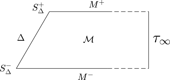
Figure 1: The region of space-time ${\mathcal{M}}$ under consideration has an internal boundary $\Delta$ and is bounded by two partial Cauchy surfaces $M^{\pm}$ which intersect $\Delta$ in the $2$-spheres $S^{\pm}_{\Delta}$ and extend to spatial infinity where they cross the cylinder $\tau_{\infty}$.

Our covariant phase space $\Gamma$ will consist of solutions $(A_{I},e^{I},{\bf A})$ to the Einstein-Maxwell equations, satisfying the above boundary conditions. As usual, to construct the symplectic structure on $\Gamma$, we begin with the (anti-symmetrized) second variation of the action (3.1). Applying the equations of motion to this second variation, one finds that the integral over ${\mathcal{M}}$ reduces to surface terms at $M^{\pm}$ and at $\Delta$. The surface term at $\tau_{\infty}$ vanishes because of the asymptotic fall-off conditions. Furthermore, expressed in terms of $\psi$ and $\chi$, the surface term at $\Delta$ turns out to be exact and thus reduces to a pair of integrals on $S_{\Delta}^{\pm}$. The integral over $M^{+}$, together with its surface term at $S_{\Delta}^{+}$ is then taken to define the symplectic structure $\Omega$ on $\Gamma$:

$$\Omega{\mid_{(A,e,{\bf A})}}\,(\delta_{1},\delta_{2}) = -\int_{M}\left(\delta_{1}A^{I}\wedge\delta_{2}e_{I}-\delta_{2}A^{I}\wedge\delta_{1}e_{I}\right)-$$

$$- \oint_{S_{\Delta}}\left(\delta_{1}\psi\,\delta_{2}m-\delta_{2}\psi\,\delta_{2}m\right)+$$

$$+ \frac{1}{2\pi}\int_{M}\left(\delta_{1}{\bf A}\wedge\delta_{2}{}^{\star}{\bf F}-\delta_{2}{\bf A}\wedge\delta_{1}{}^{\star}{\bf F}\right)+$$

$$+ \frac{1}{2\pi}\oint_{S_{\Delta}}\left(\delta_{1}\chi\,\delta_{2}{}^{\star}{\bf F}-\delta_{2}\psi\,\delta_{1}{}^{\star}{\bf F}\right)$$

for any two tangent vectors $\delta_{1}$ and $\delta_{2}$ at the phase space point $(A,e,{\bf A})$.

One can verify that, with our boundary conditions, the integral converges in spite of the logarithmic divergences at infinity and, because of field equations, it is conserved in spite of the presence of internal boundaries. More precisely, given a general solution to the field equations and for general solutions $\delta_{1}$ and $\delta_{2}$ to the linearized equations on ${\mathcal{M}}$, the integral (4.1) evaluated on a partial Cauchy slice $M$ is well-defined and independent of the choice of that slice [5, 6]. Note that this conservation would not hold had we left out the boundary term. The integral of the ‘symplectic current’ constructed from the bulk terms across $\Delta$ is compensated by the difference between the boundary terms evaluated at $M_{\pm}$ [5].

Remark: As in higher dimensions, the term ‘symplectic structure’ is somewhat of a misnomer because in the covariant phase space framework, $\Omega$ can have degenerate directions which correspond to infinitesimal gauge transformations. However, because the first homology of ${\mathcal{M}}$ is non-trivial, there is now an interesting subtlety involving the electromagnetic potential. Denote by $\tilde{\phi}_{a}$ the closed 1-form on ${\mathcal{M}}$ which can be locally expressed as the exact differential $\partial_{a}\phi$. Then, $\delta{\bf A}_{a}=\tilde{\phi}_{a}$ is a pure gauge connection from a space-time perspective because $\delta{\bf F}=d\tilde{\phi}=0$. However, this $\delta{\bf A}$ does not belong to the kernel of the symplectic structure because it is not exact. Therefore, from a phase space perspective, this is not a pure gauge connection. From now on, we will use the phase space notion of gauge. Thus, an expression will be said to be gauge invariant if it is invariant under ${\bf A}\mapsto{\bf A}+df$ for a smooth function $f$.

4.2 Angular momentum

Let $\phi^{a}$ be a vector field on ${\mathcal{M}}$ with closed orbits whose affine parameter runs between $0$ and $2\pi$ such that it is a rotational Killing vector of the asymptotic metric at infinity and coincides with the fixed rotational symmetry vector field $\varphi$ on $\Delta$. ($\phi^{a}$ is not required to be a Killing field in the bulk; indeed general metrics in our phase space do not admit any Killing field.) Diffeomorphisms generated by $\phi^{a}$ naturally induce a vector field

$$\delta_{\phi}=({\cal L}_{\phi}\,A,\,{\cal L}_{\phi}\,e,\,{\cal L}_{\phi}\,{\bf A})$$ (4.2)

on the phase space $\Gamma$. It is natural to ask whether it preserves the symplectic structure. As on any phase space, the answer is in the affirmative if and only if the 1-form $X^{(\phi)}$ on $\Gamma$ defined by

$$X^{(\phi)}(\delta)=\Omega(\delta,\delta_{\phi})$$ (4.3)

is exact, where $\delta$ is an arbitrary vector field on $\Gamma$. A direct calculation of the right hand side of (4.3) shows that this is indeed the case: $X^{(\phi)}=dJ^{(\phi)}$ where the phase space function $J^{(\phi)}$ is given, up to an additive constant, by:

$$J^{(\phi)} = \oint_{S_{\Delta}}\left[(\varphi\cdot\omega)m-\frac{1}{2\pi}(\varphi\cdot{\bf A}){}^{\star}{\bf F}\right]+$$

$$+ \oint_{S_{\infty}}\,\left[(\varphi\cdot e_{I})A^{I}+-\frac{1}{2\pi}(\varphi\cdot{\bf A}){}^{\star}{\bf F}\right]$$

$$= J_{\Delta}-J_{\infty}$$

(Because of the absence of a background geometry, the Hamiltonians generating space-time diffeomorphisms in the covariant phase space consist only of boundary terms.) The requirement that $J^{(\phi)}$ must vanish in the non-rotating BTZ solution implies that the undetermined constant must be zero. Finally, in spite of the fact that the electromagnetic potential ${\bf A}$ appears explicitly, the expression is gauge invariant.

The integral $J_{\infty}$ at infinity is the total angular momentum of the system, including contributions from matter fields outside $\Delta$. Note that, in contrast to the situation in 3+1 dimensions, this surface term contains a contribution from the Maxwell field. The evaluation of the surface term is delicate. As before, one has to first evaluate the integral on the exterior boundary of a finite region of a partial Cauchy surface and then take the limit to infinity. In the limit, the contributions from the Maxwell and the gravitational parts diverge individually but the sum is finite. Finally, it is natural to interpret the horizon integral $J_{\Delta}$ as the horizon angular momentum. As in higher dimensions [6], this interpretation is supported by various properties. In particular, if the space-time admits a rotational Killing field $\phi^{a}$ in a neighborhood of $\Delta$, then

$$J^{\rm grav}_{\Delta}\equiv J^{\rm Komar}_{\Delta}=-\frac{1}{2}\,\oint_{S_{\Delta}}\,{}^{\star}{d\phi}\,,$$ (4.5)

where $J^{\rm grav}_{\Delta}$ is the gravitational part of the horizon angular momentum $J_{\Delta}$ in (4.2). It is straightforward to check that, in the BTZ solutions, $J_{\Delta}=J$, where $J$ is the parameter in the BTZ metric. Also, as one might expect from the presence of a global Killing field $\phi$, in these solution $J_{\Delta}=J_{\infty}$ so that the Hamiltonian $J^{(\phi)}$ generating the diffeomorphism along $\phi$ vanishes identically. From general symplectic geometry considerations, it follows that this result holds also on the entire connected component of axi-symmetric solutions containing the BTZ solution. In the general non axi-symmetric case, on the other hand $J^{(\phi)}$ is non-zero and represents the angular momentum in the Maxwell field outside the horizon. Finally, the electromagnetic part of the horizon term $J_{\Delta}$ can be expressed in terms of the electric charge $Q$ and the Aharanov-Bohm charge $\tilde{Q}$ of (2.36) :

$$J_{\Delta}^{\rm em}=-\frac{1}{2\pi}\oint_{S_{\Delta}}\,(\varphi\cdot{}^{\star}{\bf F})\,{\bf A}=-\frac{1}{2\pi}Q\tilde{Q}$$ (4.6)

4.3 Energy and the first law

Following the strategy adopted for defining angular momentum, it is natural to define horizon energy as the appropriate surface term in the expression of the Hamiltonian generating time-evolution. Let us therefore begin by introducing, in each history, an ‘evolution vector field’ $t^{a}$. To qualify as a ‘time translation’, $t^{a}$ will be required to be a generator of an appropriate symmetry at the two boundaries: we will assume that it approaches a fixed time translation at spatial infinity and has the form $t^{a}=c_{{(t)}}\ell^{a}-\Omega_{{(t)}}\varphi^{a}$ on $\Delta$, where $c_{{(t)}}$ and $\Omega_{{(t)}}$ are constants on $\Delta$. It turns out to be necessary to allow $t^{a}$ to vary from one space-time to another; in the numerical relativity terminology, the vector field is allowed to be ‘live’. The asymptotic value of $t^{a}$ at spatial infinity is independent of the choice of history and defines a fixed time translation Killing field of the asymptotic metric. On the horizon, on the other hand, $c_{(t)}$ and $\Omega_{(t)}$ are allowed to vary from one space-time to another. For example, for physical reasons, in the non-rotating BTZ solution, we would like $\Omega_{(t)}$ to vanish, while in the rotating case we would like it to be non-zero. As we will see, this generalization is essential to obtain a well-defined Hamiltonian as well as the first law.

The evolution field $t^{a}$ induces a vector field $\delta_{t}$ on the phase space, given by

$$\delta_{t}=({\cal L}_{t}\,A,\,{\cal L}_{t}\,e,\,{\cal L}_{t}\,{\bf A}),$$ (4.7)

and representing infinitesimal time evolution. The key question now is whether this evolution is Hamiltonian, i.e., if $\delta_{t}$ preserves the symplectic structure $\Omega$ on $\Gamma$. As usual, this is the case if and only if the one form $X^{(t)}$ on $\Gamma$ defined by

$$X^{(t)}(\delta)=\Omega\left(\delta,\delta_{t}\right)$$ (4.8)

is closed.

We can evaluate the right-hand side of (4.8) using the expression (4.1) of the symplectic structure and simplify it using equations of motion, conditions (3.3) and (2.34) on the gravitational and electromagnetic potentials, and the fact that, on the horizon, $\delta\ell\hat{=}c_{\delta}\ell$ for some constant $c_{\delta}$. The resulting expression again involves only integrals at the boundary of space-time ${\mathcal{M}}$.

$$X^{(t)}(\delta)=X^{(t)}_{\infty}(\delta)-\kappa_{(t)}\delta a_{\Delta}-\Omega_{(t)}\delta J_{\Delta}-\Phi_{(t)}\delta Q_{\Delta},$$ (4.9)

where $X^{(t)}_{\infty}(\delta)$ involves only fields at infinity; $\kappa_{(t)}$ and $\Phi_{(t)}$ are, respectively, the surface gravity and electric potential on $\Delta$, both associated with $c_{(t)}\ell$. Using boundary conditions at infinity, we can express the term $X^{(t)}_{\infty}(\delta)$ as an exact variation. As in the case of angular momentum, the actual evaluation of this surface term is somewhat delicate: the gravitational and the electromagnetic terms diverge individually; it is only the sum that is finite. The final result is:

$$X^{(t)}_{\infty}(\delta) = \delta E^{t}_{\infty},\quad{\rm with}\quad$$

$$E^{t}_{\infty} = \frac{1}{4}\Lambda Q^{2}\omega^{2}-\frac{1}{2}Q^{2}\ln\frac{\bar{r}_{0}}{\bar{l}}(1-\Lambda\omega^{2}),$$ (4.10)

where the parameters $Q$, $\omega$ and $\bar{r}_{0}$ can be read off from the asymptotic behavior specified in Appendix B. $E^{t}_{\infty}$ is the energy at infinity corresponding to the asymptotic time translation $t^{a}$. (Again, the freedom to add a constant is eliminated by requiring that $E^{t}_{\infty}$ should yield $M$ when $t^{a}$ is chosen to be the standard time translation in non-rotating BTZ space-times.)

From (4.9) and (4.10) we conclude that the evolution along $t^{a}$ is Hamiltonian if and only if the horizon term in (4.9) is an exact variation, i.e., if and only if there exists a function $E_{\Delta}^{t}$ on the phase space, constructed from fields at the horizon, such that

$$\delta E_{\Delta}^{t}=\kappa_{(t)}\delta a_{\Delta}+\Omega_{(t)}\delta J_{\Delta}+\Phi_{(t)}\delta Q_{\Delta}.$$ (4.11)

It is natural to identify $E_{\Delta}^{t}$ as the horizon energy. Remarkably, (4.11) is precisely the statement of the first law. Thus, the first law (4.11) is the necessary and sufficient condition that the time evolution generated by the live vector field $t^{a}$ on ${\mathcal{M}}$ is Hamiltonian.

Not every live vector field $t^{a}$ considered above satisfies this condition. A vector field which does will be said to be admissible. We will show in the next section that there exists an infinite number of admissible vector fields, whence there is an infinite family of first laws. A natural question is whether one can make a canonical choice, using our knowledge of known exact solutions. We will show that the answer is in the affirmative. The horizon energy defined by this canonical live vector field will be called the horizon mass.

Remark: In contrast to the asymptotically flat case treated in higher dimensions [5, 6], in stationary space-times, the expression (4.10) of the energy at infinity does not agree with the Komar integral. In fact, the Komar integral now diverges, while our expression is finite.

5 Horizon mass

In this section, we will first introduce a systematic procedure to construct admissible vector fields and then use our knowledge of stationary, axi-symmetric black hole solutions to introduce preferred admissible vector fields on all space-times in the phase space $\Gamma$.

5.1 Admissible vector fields

Note first that (4.11) implies that $t^{a}$ is an admissible vector field only if $E_{\Delta}^{t},\kappa_{(t)}$, $\Omega_{(t)}$ and $\Phi_{(t)}$ are all functions only of the horizon parameters $(a_{\Delta},J_{\Delta},Q_{\Delta})$. Furthermore (4.11) implies that the following rather stringent condition must be met at the horizon:

$$\frac{\partial\kappa_{(t)}}{\partial J_{\Delta}}=\frac{\partial\Omega_{(t)}}{\partial a_{\Delta}}.$$ (5.1)

We will turn the argument around and use this equation to construct admissible vector fields. Let us begin by fixing a ‘suitably regular’ function $\kappa_{0}(a_{\Delta},J_{\Delta},Q_{\Delta})$ of the horizon parameters. Now, given a general solution, the surface gravity ${\kappa_{(\ell)}\,}$ of the null generator $\ell$ will not equal $\kappa_{0}$. However, there will be a unique constant $c$ such that $\kappa_{(c\ell)}=\kappa_{0}$. Next, we find a constant $\Omega_{(t)}$ by integrating (5.1) with respect to $a_{\Delta}$:

$$\Omega_{t}=\int_{\infty}^{a}\frac{\partial\kappa_{0}}{\partial J_{\Delta}}\,{d}a_{\Delta}\,+\,F(Q_{\Delta},J_{\Delta}),$$ (5.2)

where $F$ is an arbitrary function of the two parameters. (The qualification ‘suitably regular’ above is meant to ensure that the integral on the right is well-defined.) Finally, we can fix the arbitrariness in $\Omega_{(t)}$ by imposing the following physical requirement:

$$\lim_{\stackrel{{\scriptstyle J_{\Delta},Q_{\Delta}=\mbox{{\scriptsize}{const.}}}}{{a_{\Delta}\rightarrow\infty}}}\Omega_{(t)}=0.$$

Now, in any given solution in the phase space, we choose any evolution vector field $t^{a}$ such that it tends to the fixed asymptotic time-translation at infinity and satisfies $t^{a}\widehat{=}c\ell^{a}-\Omega_{(t)}\varphi^{a}$ on $\Delta$. It is straightforward to check that, by construction, this evolution vector field is admissible if the Maxwell field of the solution under consideration vanishes on $\Delta$.

If the Maxwell field on $\Delta$ is non-zero, we must also ensure that the Maxwell gauge is fixed appropriately for (4.11) to hold. Recall first that in an adapted gauge, the Maxwell potential ${\bf A}$ is such that $\Phi_{\ell}\widehat{=}-{\bf A}_{a}\ell^{a}$ is constant on $\Delta$. However, the value of the constant, i.e., its possible dependence on the horizon parameters, is still completely unconstrained. Equation (4.11) imposes severe restrictions on this choice: $\Phi_{(t)}\equiv\Phi_{(c\ell)}$ must satisfy

$$\frac{\partial\Phi_{(t)}}{\partial a_{\Delta}}=\frac{\partial\kappa_{(t)}}{\partial Q_{\Delta}},$$

$$\frac{\partial\Phi_{(t)}}{\partial J_{\Delta}}=\frac{\partial\Omega_{(t)}}{\partial Q_{\Delta}}.$$ (5.3)

Again, we can just use this condition to constrain $\Phi_{(t)}$: setting $\kappa_{(t)}=\kappa_{0}$ and using $\Omega_{(t)}$ determined above, we can simply integrate these equations to determine $\Phi_{(t)}$ up to an additive function $F(Q)$ of the charge, $Q_{\Delta}$. In 3+1 dimensions, there was a natural way to fix this freedom [4, 6]: One could just impose the physical requirement that $\Phi_{(t)}$ should vanish in the limit of large areas, with fixed charge and angular momentum. Unfortunately, in 2+1 dimensions this strategy is not viable because now, in presence of a non-zero charge, the potential diverges at spatial infinity! Therefore now $\Phi_{(t)}$ is not completely determined on $\Delta$. The only physical restriction we impose on $F(Q)$ is through

$$\lim_{\stackrel{{\scriptstyle J_{\Delta},a_{\Delta}=\mbox{{\scriptsize const.}}}}{{Q_{\Delta}\rightarrow 0}}}\Phi_{(t)}=0,$$ (5.4)

which only determines the value of $F(Q)$ at $Q=0$.

Note, however, that the remaining freedom is irrelevant for the purpose of defining admissible vector fields: the vector fields $t^{a}$ constructed above are admissible for every choice of $\Phi_{(t)}$ satisfying (5.1). However, the choice of $\Phi_{(t)}$ will, in general, enter the expression of the horizon energy $E^{t}_{\Delta}$ which is obtained by integrating (4.11).

5.2 Preferred admissible vector fields

In this section, we will indicate how one can use the known solutions to fix $\kappa_{0}$ and $\Phi_{(t)}$ in a ‘canonical fashion’. The resulting $E^{t}_{\Delta}$ can be naturally interpreted as the horizon mass. Several subtleties arise in presence of a non-zero charge and angular momentum. Therefore we will divide the discussion into three cases.

5.2.1 The case with ${\bf F}_{ab}\widehat{=}0$

Let us suppose that the Maxwell field vanishes on the horizon. Then we only have to choose a function $\kappa_{0}$ of the horizon parameters $a_{\Delta},J_{\Delta}$. However, in this case, there is a unique BTZ black hole solution for each choice of these two parameters. Therefore, it is natural to set $\kappa_{0}=\kappa_{(t)}^{\rm BTZ}$, where $t^{a}$ is the canonical time-translation Killing field of the BTZ black hole:

$$\kappa_{0}\equiv\kappa_{(t)}=-\frac{\Lambda a_{\Delta}}{2\pi}-\frac{2\pi J_{\Delta}^{2}}{a_{\Delta}^{3}}.$$ (5.5)

Our construction of Section 5.1 implies

$$\Omega_{(t)}=\frac{2\pi J_{\Delta}}{a_{\Delta}^{2}}.$$ (5.6)

We can now integrate out the first law to obtain the expression of the horizon energy up to an undetermined additive constant. We eliminate this freedom through the physical requirement: $\lim_{a_{\Delta}\rightarrow 0}E_{\Delta}^{t}=0$ for non-rotating isolated horizons. The resulting horizon mass is given as a function of the horizon parameters as:

$$M_{\Delta}=-\frac{1}{4\pi}\Lambda a_{\Delta}^{2}+\frac{\pi J_{\Delta}^{2}}{a_{\Delta}^{2}}.$$ (5.7)

The functional form of $M_{\Delta}$ is the same as that in the BTZ family. However, (5.7) was not simply postulated but derived systematically from Hamiltonian considerations and applies to all isolated horizons including those which may admit electromagnetic radiation in the exterior region, away from $\Delta$. In presence of such radiation, $M_{\Delta}$ will not equal the mass at infinity.

5.2.2 Charged, non-rotating horizons

Next, let us consider non-rotating horizons with electric charge. For brevity, we will treat this as a sub-case (corresponding to $\omega=0$) of the Clément solution. The metric and the Maxwell field of this solution were given in section 2.1. The corresponding electromagnetic potential, satisfying the boundary conditions of Appendix B, is given by

$${\bf A}=Q\ln(\frac{r}{l})dv.$$ (5.8)

Using the Killing field $t=\partial_{v}$ as the evolution field, it is again natural to set $\kappa_{0}=\kappa_{(t)}$ and $\Phi_{(t)}\widehat{=}-{\bf A}_{a}t^{a}$. Thus, we now have:

$$\kappa_{0}\equiv\kappa_{(t)}=-\Lambda\frac{a_{\Delta}}{2\pi}-\frac{Q_{\Delta}^{2}}{2a_{\Delta}}.$$ (5.9)

and

$$\Phi_{(t)}=-Q_{\Delta}\ln\frac{a_{\Delta}}{a_{0}},$$ (5.10)

where $a_{0}=2\pi l$. Thus, we have used our boundary conditions at spatial infinity to determine $\Phi_{t}$ uniquely in these solutions. Since angular momentum vanishes, $\Omega_{t}=0$

For general non-rotating weakly isolated horizons, therefore, we select the canonical evolution vector fields and electromagnetic scalar potential by demanding that the dependence of $\kappa_{0}$ and $\Phi_{t}$ on $a_{\Delta}$ and $Q_{\Delta}$ be fixed as in Equations (5.9) and (5.10), and $\Omega_{t}$ should vanish. Then, it is straightforward to integrate the first law to obtain the horizon mass. We obtain:

$$M_{\Delta}=-\frac{\Lambda a_{\Delta}^{2}}{4\pi}-\frac{1}{2}Q_{\Delta}^{2}\ln\frac{a_{\Delta}}{a_{0}}.$$ (5.11)

Again, this formula now holds for arbitrary non-rotating weakly isolated horizons $\Delta$.

5.2.3 Charged rotating black hole.

Finally, let us consider the general case. We can now use the general Clément solution to fix $\kappa_{0}$ and $\Omega_{(t)}$.

As in the charged, non-rotating case, we need to specify the electromagnetic vector potential ${\bf A}_{a}$. The potential satisfying our boundary conditions as well as conditions (5.1) which are necessary for the first law to hold is given by:

$${\bf A}=Q\ln\frac{r}{\bar{l}}(dv-\omega d\phi)+\frac{1}{2}Q\omega^{2}\Lambda dv.$$ (5.12)

Next, let us express the horizon parameters $a_{\Delta},Q_{\Delta}$ and $J_{\Delta}$ in terms of the parameters $\omega,Q,\bar{r}_{0}$ that appear in the solution:

$$a_{\Delta} = \frac{2\pi r_{\Delta}}{\sqrt{1+\omega^{2}\Lambda}}$$

$$Q_{\Delta} = Q$$

$$J_{\Delta} = -\omega\left(\frac{\Lambda a_{\Delta}^{2}}{2\pi}+\frac{1}{2}Q_{\Delta}^{2}+Q_{\Delta}^{2}\ln\frac{a_{\Delta}}{2\pi l}\right),$$ (5.13)

where $r_{\Delta}$ is given by $N(r=r_{\Delta})=0$. (The parameter $\bar{r}_{0}$ enters the expression of the area through this condition.)

Now we can calculate the surface gravity $\kappa_{(t)}$ and the electric potential $\Phi_{(t)}$ corresponding to the stationary Killing field $t^{a}$ of the Clément solution:

$$\kappa_{(t)} = -\left(\frac{\Lambda a_{\Delta}}{2\pi}+\frac{Q_{\Delta}^{2}}{2a_{\Delta}}\right)(1+\omega^{2}\Lambda),$$ (5.14)

$$\Phi_{(t)} = -Q_{\Delta}\ln\frac{a_{\Delta}}{a_{0}}(1+\omega^{2}\Lambda)-\frac{1}{2}Q_{\Delta}\omega^{2}\Lambda,$$ (5.15)

where, as before, $a_{0}=2\pi l$.

In a general solution in the phase space, then, we set $\kappa_{0}=\kappa_{(t)}$ given above. Our procedure of Section 5.1 provides the required $\Omega_{(t)}$:

$$\Omega_{(t)}=-N^{\phi}(r=r_{\Delta})=-\omega\Lambda.$$ (5.16)

The triplet $\kappa_{(t)},\Omega_{(t)},\Phi_{(t)}$ can now be used to construct preferred admissible vector fields and by integrating the corresponding first law, we obtain the expression of the horizon mass:

$$M_{\Delta}=-\frac{\Lambda a_{\Delta}^{2}}{4\pi}-\frac{1}{2}Q_{\Delta}^{2}\ln\frac{a_{\Delta}}{a_{0}}+\frac{1}{2}\frac{\Lambda J_{\Delta}^{2}}{\frac{\Lambda a_{\Delta}^{2}}{2\pi}+\frac{1}{2}Q_{\Delta}^{2}+Q_{\Delta}^{2}\ln\frac{a_{\Delta}}{a_{0}}}$$ (5.17)

where we have again eliminated an undetermined constant by requiring that every non-rotating, uncharged horizon should have vanishing mass in the limit of vanishing area. This is our general expression of the horizon mass.

Finally, we can compare our formula for the energy of the horizon with the energy at infinity —Eq.(4.10). It is easy to check that in the case of Clément’s solution, the two expressions are equal to each other, just as one might expect from results in 3+1 dimensions. General symplectic arguments [6, 15] now imply that this equality between our horizon mass and the mass at infinity must continue to hold for all stationary space-times in the connected component of the phase-space containing Clément (or, equivalently, BTZ) solutions.

6 Horizon geometry

In this section, we examine geometrical structures on $\Delta$ and analyze their interplay with the field equations. As mentioned in the Introduction, this section can be read independently of the last three.

The section is divided into four parts. In the first, we will show that every non expanding horizon is naturally equipped with an intrinsic derivative operator ${\cal D}$. In the second, we will turn to weakly isolated horizons and, using field equations, isolate the freely specifiable data on $\Delta$. In the third, we will show that every non-extremal weakly isolated horizon admits a natural foliation (irrespective of whether it is axi-symmetric, i.e., type I in the terminology of section 2.3). In the last sub-section we strengthen the definition of weak isolation to introduce the notion of isolated horizons. While a non-expanding horizon $\Delta$ can be made weakly isolated by suitably choosing $[\ell]$ in infinitely many inequivalent ways, generically, it admits a unique $[\ell]$ which makes it isolated.

6.1 A natural derivative operator

Let $\Delta$ be a non-expanding horizon. Had it been space-like or time-like, its intrinsic metric would have selected a unique (torsion-free) derivative operator. However, since it is null, there are infinitely many derivative operators which are compatible with it. Nonetheless, because $\Delta$ is expansion and shear-free, as in higher dimensions [5], the full space-time derivative operator $\nabla$ induces a preferred intrinsic derivative ${\cal D}$ on it. Given a vector field $X^{a}$ or a 1-form $f_{a}$, on $\Delta$, we have:

$$Y^{a}{\cal D}_{a}X^{b}\widehat{=}Y^{a}\nabla_{a}{\bar{X}}^{b},\quad{\rm and}\quad Y^{a}Z^{b}{\cal D}_{a}f_{b}\widehat{=}Y^{a}Z^{b}\nabla_{a}{\bar{f}}_{b}\,,$$ (6.1)

where $Y^{a},Z^{a}$ are arbitrary vector fields tangential to $\Delta$ and $\bar{X}^{a}$ and ${\bar{f}}_{a}$ are arbitrary smooth extensions of $X^{a}$ and $f_{a}$ to a space-time neighborhood of $\Delta$. It is easy to check that ${\cal D}$ is well-defined: the right hand sides of the two equations are independent of the choice of extension and the right hand side of the first equation is again tangential to $\Delta$. Since $\nabla_{a}g_{bc}=0$ in space-time, ${\cal D}_{a}q_{bc}\widehat{=}0$ on $\Delta$; as expected, ${\cal D}$ is compatible with $q_{bc}$.

What information does ${\cal D}$ have beyond that contained in the degenerate metric $q_{ab}$ on $\Delta$? The action of ${\cal D}$ on tensors is completely determined by that on all 1-forms defined intrinsically on $\Delta$. Let $f$ be a 1-form satisfying $f\cdot\ell\widehat{=}0$ and ${\cal L}_{\ell}f\widehat{=}0$. Then it is easy to verify that the action of ${\cal D}$ on $f$ can be expressed just in terms of exterior and Lie derivatives:

$$2{\cal D}_{a}f_{b}=2{\cal D}_{[a}f_{b]}+{\cal L}_{\hat{f}}\,q_{ab}$$ (6.2)

where the vector field $\hat{f}^{a}=m^{a}m^{b}f_{b}$ is independent of the choice of the unit space-like vector $m^{a}$ tangential to $\Delta$. Thus, the action of ${\cal D}$ on these 1-forms is determined by $q_{ab}$. Therefore, ${\cal D}$ is completely determined by its action ${\cal D}_{a}n_{b}=:S_{ab}$ on 1-forms $n$ satisfying $n\cdot\ell=-1$. Without loss of generality, we can assume that $n$ satisfies, in addition,

$${\cal L}_{\ell}\,n\widehat{=}0\quad{\rm and}\quad dn\widehat{=}0$$ (6.3)

on $\Delta$. Then $S_{ab}$ is symmetric. Since $dn\widehat{=}0$, we have $n=-dv$ for some function $v$ on $\Delta$ satisfying ${\cal L}_{\ell}v=1$. The $v={\rm const}$ cross-sections will be assumed to be topologically $S^{1}$ and denoted $\tilde{\Delta}$.

Now,

$$\ell^{b}S_{ab}\widehat{=}-n_{b}{\cal D}_{a}\ell^{b}\widehat{=}-n_{b}\nabla\!_{{\mathchoice{\vtop{\halign{#\cr$\textstyle{a}$\crcr\kern-1.20552pt\nointerlineskip\cr{\tiny\leftarrowfill}\crcr}}}{\vtop{\halign{#\cr$\textstyle{a}$\crcr\kern-1.20552pt\nointerlineskip\cr{\tiny\leftarrowfill}\crcr}}}{\vtop{\halign{#\cr\hfil$\scriptstyle{a}$\hfil\crcr\kern 1.20552pt\nointerlineskip\cr{\tiny\leftarrowfill}\crcr}}}{\vtop{\halign{#\cr\hfil$\scriptstyle{a}$\hfil\crcr\kern 1.20552pt\nointerlineskip\cr{\tiny\leftarrowfill}\crcr}}}}\vphantom{a}}\ell^{b}\widehat{=}\omega_{a}$$ (6.4)

Thus, part of the ‘new’ information in ${\cal D}$ is contained in the 1-form $\omega$ of Section 2.1. The rest is contained in the projection $\tilde{\mu}$ of $S_{ab}$ on $\tilde{\Delta}$: $\tilde{\mu}:\widehat{=}\tilde{m}^{a}\tilde{m}^{b}{\cal D}_{a}n_{b}$ where $\tilde{m}^{a}$ is the unit vector field tangential to $\tilde{\Delta}$. This function $\tilde{\mu}$ is the ‘transversal expansion’ of $n$ (see Appendix A).

Following the terminology used in higher dimensions [10], we will refer to the pair $(q,{\cal D})$ as the intrinsic geometry of $\Delta$. Thus, the intrinsic geometry is determined by a triplet $(m^{a},\omega_{a},\tilde{\mu})$ on $\Delta$ for any choice of $n$ satisfying (6.3).

6.2 Field equations and ‘free data’ on a weakly
isolated horizon

Consider a weakly isolated horizon $(\Delta,[\ell])$. In this sub-section we will analyze the restrictions imposed by field equations on the intrinsic geometry of $\Delta$ and extract the free-data that suffices to determine this geometry.

We already know that the pair $(q,{\cal D})$ satisfies

$$q_{ab}\ell^{b}\widehat{=}0;\quad{\cal L}_{\ell}\,q_{ab}\widehat{=}0;\quad{\cal D}_{a}q_{bc}\widehat{=}0;\quad{\cal D}_{a}\ell^{b}\widehat{=}\omega_{a}\ell^{b};\quad{\cal L}_{\ell}\,\omega\widehat{=}0;$$ (6.5)

and Equations (6.2) and (6.4). We now want to analyze the further constraints imposed by the full field equations: $E_{ab}:=R_{ab}-\frac{1}{2}Rg_{ab}+\Lambda g_{ab}-T_{ab}\widehat{=}0$. We already saw in Section 2 that weak isolation implies $R_{ab}\ell^{a}\ell^{b}\widehat{=}0$ and $R_{ab}\ell^{a}m^{b}\widehat{=}0$. Hence these projections of the field equations do not further constrain the horizon geometry; they only restrict the matter fields at the horizon. It turns out that the projections $E_{ab}n^{a}\ell^{b}\widehat{=}0$ and $E_{ab}n^{a}m^{b}\widehat{=}0$ dictate the propagation of $\omega$ (or, the Newman-Penrose spin coefficients $\epsilon$ and $\pi$ of Appendix A) off $\Delta$ while $E_{ab}n^{a}n^{b}\widehat{=}0$ dictates the propagation of $\tilde{\mu}$ off $\Delta$. Thus, these equations do not constrain the intrinsic horizon geometry in any way. (For details, see Appendix A.1.)

The only new constraint comes from the equation $E_{ab}\tilde{m}^{a}\tilde{m}^{b}\widehat{=}0$. Had $\Delta$ been a space-like surface, the analogous equations would have given the evolution equations. In the present case they also dictate an ‘evolution’ —that of $\tilde{\mu}$— but now within $\Delta$. We have:

$${\cal L}_{\ell}\,\tilde{\mu}\widehat{=}-{\kappa_{(\ell)}\,}\tilde{\mu}+\tilde{m}^{a}\tilde{m}^{b}{\cal D}_{(a}\tilde{\omega}_{b)}+(\tilde{m}^{a}\tilde{\omega}_{a})^{2}+\frac{1}{2}\tilde{m}^{a}\tilde{m}^{b}t_{ab}.$$ (6.6)

where $\tilde{\omega}_{a}=\tilde{m}_{a}\tilde{m}^{b}\omega_{b}$ is the projection of $\omega$ on $\tilde{\Delta}$ and $t_{ab}=(T_{ab}+(2\Lambda-T)g_{ab})$. This exhausts the field equations.

We can now specify the freely specifiable part of the horizon geometry. Fix a 2-manifold $\Delta$, topologically $S^{1}\times{\mbox{\rm$\mbox{I}\!\mbox{R}$}}$, and equip it with a vector field $\ell$ along the IR direction. Fix a foliation by circles labeled by $v={\rm const}$, where ${\cal L}_{\ell}\,v=1$. On any one cross-section, $\tilde{\Delta}$, fix a function $\tilde{\mu}$ and 1-forms $m$ and $\omega$ such that $m$ is nowhere vanishing, $m\cdot\ell=0$, and $\omega\cdot\ell={\kappa_{(\ell)}\,}$, where ${\kappa_{(\ell)}\,}$ is a constant. This is the free data. ‘Evolve’ it to all of $\Delta$ through ${\cal L}_{\ell}\,m=0$, ${\cal L}_{\ell}\,\omega=0$ and (6.6), for a given $t_{ab}$ on $\Delta$. Then the triplet $(m,\omega,\tilde{\mu})$ on $\Delta$ provides us with the intrinsic geometry of a weakly isolated horizon.

Finally, under the mild assumption, ${\cal L}_{\ell}\,R_{{\mathchoice{\vtop{\halign{#\cr$\textstyle{ab}$\crcr\kern-1.20552pt\nointerlineskip\cr{\tiny\leftarrowfill}\crcr}}}{\vtop{\halign{#\cr$\textstyle{ab}$\crcr\kern-1.20552pt\nointerlineskip\cr{\tiny\leftarrowfill}\crcr}}}{\vtop{\halign{#\cr\hfil$\scriptstyle{ab}$\hfil\crcr\kern 1.20552pt\nointerlineskip\cr{\tiny\leftarrowfill}\crcr}}}{\vtop{\halign{#\cr\hfil$\scriptstyle{ab}$\hfil\crcr\kern 1.20552pt\nointerlineskip\cr{\tiny\leftarrowfill}\crcr}}}}\vphantom{ab}}\widehat{=}0$, we can integrate (6.6) to obtain:

$$\tilde{\mu}=e^{-{\kappa_{(\ell)}\,}v}\tilde{\mu}^{0}+\frac{1}{{\kappa_{(\ell)}\,}}\left[\tilde{m}^{a}\tilde{m}^{b}{\cal D}_{(a}\tilde{\omega}_{b)}+(\tilde{m}^{a}\tilde{\omega}_{a})^{2}+\frac{1}{2}\tilde{m}^{a}\tilde{m}^{b}t_{ab}\right]$$ (6.7)

if ${\kappa_{(\ell)}\,}{\not\!\!\widehat{=}}0$ and

$$\tilde{\mu}=\tilde{\mu}^{0}+\left[\tilde{m}^{a}\tilde{m}^{b}{\cal D}_{(a}\tilde{\omega}_{b)}+(\tilde{m}^{a}\tilde{\omega}_{a})^{2}+\frac{1}{2}\tilde{m}^{a}\tilde{m}^{b}t_{ab}\right]v$$ (6.8)

if ${\kappa_{(\ell)}\,}\widehat{=}0$, where ${\cal L}_{\ell}\,\tilde{\mu}^{0}\widehat{=}0$. These solutions bring out the generalization entailed in considering weakly isolated horizons in place of Killing horizons: now, even the intrinsic geometry on the horizon (as defined above) can be time-dependent. In spite of this, the zeroth and first laws hold on any weakly isolated horizon.

6.3 Good cuts of non-extremal weakly isolated horizon

As in higher dimensions [10], every non-extremal weakly isolated horizon admits a natural foliation. However, because the Weyl tensor vanishes in 3 dimensions, and the first homology of $\Delta$ is now non-trivial, the construction is now somewhat different.

Recall first that every non-expanding horizon $\Delta$ carries a natural closed 1-form $\underline{m}_{a}$. Since $d\underline{m}\widehat{=}0$, $\underline{m}$ generates a class in $H^{1}(\Delta)$, the first cohomology of $\Delta$. Since $\Delta$ is isomorphic to $S^{1}\times{\mbox{\rm$\mbox{I}\!\mbox{R}$}}$, we have:

$$H^{1}(\Delta)=H^{0}(S^{1})={\mbox{\rm$\mbox{I}\!\mbox{R}$}}.$$ (6.9)

Since the integral of $\underline{m}$ over any cross section yields $-2\pi R_{\Delta}$, $\underline{m}$ is not in the zero class of $H^{1}(\Delta)$. Next, recall that the 1-form $\omega$ on $\Delta$ is also closed. Therefore, it must be of the form

$$\omega_{a}=C\underline{m}_{a}+\partial_{a}\psi,$$ (6.10)

for some constant $C\in{\mbox{\rm$\mbox{I}\!\mbox{R}$}}$ and some function $\psi$ on $\Delta$. The function $\psi$ can now be used to define a preferred foliation of the horizon. Since

$${\cal L}_{\ell}\,\psi=\ell^{a}\omega_{a}=\kappa_{(\ell)}\,,$$ (6.11)

with $\kappa_{(\ell)}$ constant on the horizon, the lines $\psi={\rm const.}$ define a foliation of $\Delta$ provided $\kappa_{(\ell)}$ is non-zero. If the vector fields $[\ell]$ are complete, as for example in stationary black holes, the leaves of the foliation are guaranteed to be topologically $S^{1}$.

In the Newman-Penrose type framework of Appendix A, the preferred foliation is characterized by the fact that the spin-coefficient $\pi$ is constant on each leaf. Therefore, if the underlying space-time is axi-symmetric in a neighborhood of $\Delta$, the foliation coincides with the integral curves of the rotational Killing vector. In BTZ space-times, $\omega$ is given by (2.20), $d\psi\widehat{=}-{\kappa_{(\ell)}\,}n={\kappa_{(\ell)}\,}dv$, whence $\psi\widehat{=}{\kappa_{(\ell)}\,}v$, where $v$ is the Eddington-Finkelstein-like coordinate (see (2.1).

6.4 Isolated horizons and uniqueness of $[\ell]$

Let $\Delta$ be a non-expanding horizon. Fix any cross-section, choose any null normal to $\Delta$ on the cross-section and propagate it by the geodesic equation to obtain a null normal $\ell_{0}$ on $\Delta$. Then $(\Delta,[\ell_{0}])$ is an extremal weakly isolated horizon. Denote by $v_{0}$ its affine parameter. Set

$$\ell^{a}\widehat{=}{\kappa_{(\ell)}\,}\,(v_{0}-B)\,\ell_{0}^{a}$$ (6.12)

where ${\kappa_{(\ell)}\,}$ is a non-zero constant and ${\cal L}_{\ell}B\widehat{=}0$. It is straightforward to check that $\ell$ is a null normal with surface gravity ${\kappa_{(\ell)}\,}$ and every null normal with surface gravity ${\kappa_{(\ell)}\,}$ arises in this way. Similarly, any null normal with zero surface gravity is given by

$$\ell^{\prime a}\widehat{=}\left(\frac{1}{A}\right)\ell^{a}_{0}$$ (6.13)

for some function $A$ satisfying ${\cal L}_{\ell_{0}}\,A\widehat{=}0$. To summarize, simply by restricting the null normals $\ell$ to lie in a suitably chosen equivalence class $[\ell]$, from any given non-expanding horizon $\Delta$, we can construct a weakly isolated horizon $(\Delta,[\ell])$ which is either extremal or non-extremal. However, because of the arbitrary functions involved in (6.13) and (6.12), there is an infinite dimensional freedom in this construction.

It is natural to ask if this freedom can be reduced by strengthening the notion of isolation. The answer is in the affirmative.

Definition 3 An isolated horizon $(\Delta,[\ell])$ consists of a non-expanding horizon $\Delta$ equipped with an equivalence class $[\ell]$ of null normals satisfying

$$({\cal D}_{a}\,{\cal L}_{\ell}-{\cal L}_{\ell}\,{\cal D}_{a})X^{b}\widehat{=}0$$ (6.14)

for all vector fields $X$ tangential to $\Delta$. As before, $\ell$ is equivalent to $\ell^{\prime}$ if and only if $\ell^{\prime}=c\ell$ for some positive constant $c$ and if condition (6.14) holds for one null normal $\ell$, it holds for all null normals in $[\ell]$. If a non-expanding horizon $\Delta$ admits a normal $\ell$ satisfying (6.14), we will say its geometry admits an isolated horizon structure.

Before analyzing the remaining freedom in the choice of $[\ell]$, let us examine the difference between weakly isolated and isolated horizons. Note first that the weak isolation condition can be written as

$$({\cal D}_{a}\,{\cal L}_{\ell}-{\cal L}_{\ell}\,{\cal D}_{a})\ell^{b}\widehat{=}0\ .$$

Thus, the present strengthening of that notion asks that the commutator of ${\cal D}$ and ${\cal L}_{\ell}$ vanish on all vector fields on $\Delta$, not just on $\ell$. Since the information in ${\cal D}$ (beyond $q_{ab}$) is contained in the pair $(\omega,\tilde{\mu})$, the additional condition is precisely ${\cal L}_{\ell}\,\tilde{\mu}\widehat{=}0$. (While $\tilde{\mu}$ depends on the choice of cross sections $\tilde{\Delta}$,  $({\cal L}_{\ell}\,\tilde{\mu})$ does not.) Next, it is straightforward to check that, on any isolated horizon, the pull-back of the full space-time curvature is time-independent: ${\cal L}_{\ell}\,R_{{\mathchoice{\vtop{\halign{#\cr$\textstyle{ab}$\crcr\kern-1.20552pt\nointerlineskip\cr{\tiny\leftarrowfill}\crcr}}}{\vtop{\halign{#\cr$\textstyle{ab}$\crcr\kern-1.20552pt\nointerlineskip\cr{\tiny\leftarrowfill}\crcr}}}{\vtop{\halign{#\cr\hfil$\scriptstyle{ab}$\hfil\crcr\kern 1.20552pt\nointerlineskip\cr{\tiny\leftarrowfill}\crcr}}}{\vtop{\halign{#\cr\hfil$\scriptstyle{ab}$\hfil\crcr\kern 1.20552pt\nointerlineskip\cr{\tiny\leftarrowfill}\crcr}}}}\vphantom{ab}}\widehat{=}0$. (Since $R_{{\mathchoice{\vtop{\halign{#\cr$\textstyle{a}$\crcr\kern-1.20552pt\nointerlineskip\cr{\tiny\leftarrowfill}\crcr}}}{\vtop{\halign{#\cr$\textstyle{a}$\crcr\kern-1.20552pt\nointerlineskip\cr{\tiny\leftarrowfill}\crcr}}}{\vtop{\halign{#\cr\hfil$\scriptstyle{a}$\hfil\crcr\kern 1.20552pt\nointerlineskip\cr{\tiny\leftarrowfill}\crcr}}}{\vtop{\halign{#\cr\hfil$\scriptstyle{a}$\hfil\crcr\kern 1.20552pt\nointerlineskip\cr{\tiny\leftarrowfill}\crcr}}}}\vphantom{a}b}\ell^{b}\widehat{=}0$, it follows that $R_{{\mathchoice{\vtop{\halign{#\cr$\textstyle{ab}$\crcr\kern-1.20552pt\nointerlineskip\cr{\tiny\leftarrowfill}\crcr}}}{\vtop{\halign{#\cr$\textstyle{ab}$\crcr\kern-1.20552pt\nointerlineskip\cr{\tiny\leftarrowfill}\crcr}}}{\vtop{\halign{#\cr\hfil$\scriptstyle{ab}$\hfil\crcr\kern 1.20552pt\nointerlineskip\cr{\tiny\leftarrowfill}\crcr}}}{\vtop{\halign{#\cr\hfil$\scriptstyle{ab}$\hfil\crcr\kern 1.20552pt\nointerlineskip\cr{\tiny\leftarrowfill}\crcr}}}}\vphantom{ab}}$ is Lie-dragged by every null normal, $f\ell^{a}$, to $\Delta$.) Thus, on an isolated horizon, the restriction that led us to the solution (6.7) and (6.8) for $\tilde{\mu}$ is automatically satisfied. Therefore, in the non-extremal case, $\tilde{\mu}^{0}$ of (6.7) vanishes while in the extremal case the quantity in the square brackets in (6.8) must vanish. In both cases, the freely specifiable data of Section 6.2 is restricted; $\tilde{\omega}$ and $\tilde{\mu}$ can not be specified freely on a cross-section $\tilde{\Delta}$, but are constrained.

Finally, let us analyze the issue of existence and uniqueness of $[\ell]$. Let $\Delta$ be a non-expanding horizon. We can always choose a null normal $\ell$ such that $(\Delta,[\ell])$ is a non-extremal, weakly isolated horizon. Let us further suppose that $(\Delta,[\ell])$ is not already an isolated horizon, i.e., ${\cal L}_{\ell}\,\tilde{\mu}\not\!\!\widehat{=}0$ and ask if we can find another null normal $\ell^{\prime}=f\ell$ such that $(\Delta,[\ell^{\prime}])$ is isolated. Now, using the definition of weak isolation, it is straightforward to check:

$$[{\cal L}_{\ell}\,\,,{\cal D}]_{a}K_{b}\widehat{=}C_{ab}{}^{c}K_{c}\quad{\rm where}\quad C_{ab}{}^{c}\widehat{=}-Nq_{ab}\,\ell^{c}$$ (6.15)

for any 1-form $K_{b}$ on $\Delta$. The function $N$ is given by $N\widehat{=}{\cal L}_{\ell}\,\tilde{\mu}$. Under the rescaling $\ell^{\prime}\widehat{=}f\ell$, we have

$$(N^{\prime}-N)q_{ab}\widehat{=}2\omega_{(a}{\cal D}_{b)}f+{\cal D}_{a}{\cal D}_{b}f$$ (6.16)

By transvecting this equation with $\ell^{b}$ we obtain

$${\cal D}_{a}({\cal L}_{\ell}\,f+{\kappa_{(\ell)}\,}f)\widehat{=}0$$ (6.17)

which implies

$$f\widehat{=}Be^{-{\kappa_{(\ell)}\,}v}+\frac{\kappa_{(\ell^{\prime})}}{{\kappa_{(\ell)}\,}},\quad{\rm with}\,\,\,{\cal L}_{\ell}\,B\widehat{=}0.$$ (6.18)

Thus, the key question now is: Does there exist a function $B$ such that $N^{\prime}\widehat{=}0$? Substituting for $f$ in (6.16) and using the expression (6.7) of $\mu$, we conclude that $N^{\prime}$ vanishes if and only if B satisfies

$${\bf M}\cdot B:=[\tilde{{\cal D}}^{2}+2\tilde{\pi}\tilde{{\cal D}}+\tilde{\cal D}\tilde{\pi}+\tilde{\pi}^{2}+\tilde{m}^{a}\tilde{m}^{b}R_{ab}]B\widehat{=}\kappa_{(\ell^{\prime})}\tilde{\mu}^{0}$$ (6.19)

on any cross-section $\tilde{\Delta}$ of $\Delta$, where $\tilde{m}^{a}$ is the unit vector field tangential to $\tilde{\Delta}$, $\tilde{{\cal D}}:=\tilde{m}^{a}{\cal D}_{a}$ and $\tilde{\pi}:=\tilde{m}^{a}\omega_{a}$. Note that, given any cross-section $\tilde{\Delta}$, the operator is completely determined by the non-expanding horizon geometry $(q_{ab},{\cal D})$.

We will say that the horizon geometry is generic if the operator ${\bf M}$ has trivial kernel. In this case, $B={\bf M}^{-1}(\kappa_{(\ell^{\prime})}\tilde{\mu}^{0})$ is the unique solution to (6.19), where, without loss of generality, we have assumed that (the $v$-dependence of) $f$ was so chosen that $\kappa_{(\ell^{\prime})}$ is non-zero. Thus, every generic non-expanding horizon admits a unique $[\ell]$ such that $(\Delta,[\ell])$ is isolated horizon. Furthermore, this isolated horizon is non-extremal.

What happens if the horizon geometry is non-generic? In this case, Eq (6.19) implies that if we choose $B$ to belong to the kernel of ${\bf M}$, then $(\Delta,[\ell^{\prime}])$ is an extremal isolated horizon. Thus, in contrast to the situation in higher dimensions, every non-expanding horizon admits an isolated horizon structure. However, in the non-generic case, uniqueness is not assured a priori; it may be possible to choose another null normal $\ell^{\prime\prime}$ such that $(\Delta,[\ell^{\prime\prime}])$ is an isolated horizon. However, assuming that $\Delta$ admits an extremal isolated horizon structure and repeating the analysis starting from (6.16), it is easy to verify that: i) $\Delta$ can not admit a distinct extremal isolated horizon structure; and, ii) If it also admits a non-extremal isolated horizon structure, then it admits a foliation on which both null normals ($\ell^{a}$ and $n^{a}$) have zero expansions. This is an extremely special situation.

To summarize, in contrast to higher dimensions, every non-expanding horizon admits an isolated horizon structure which furthermore is unique except in extremely special cases.

7 Discussion

In this paper, we introduced the notion of non-expanding, weakly isolated and isolated horizons in 2+1-dimensional gravity (Sections 2 and 6), analyzed geometry of these horizons (Sections 2 and 6), and extended the zeroth and first laws of black hole mechanics to weakly isolated horizons (Sections 3, 4 and 5). The methods used were the same as those employed in higher dimensions [5, 6, 10] and the overall results are also analogous. In particular, the first law again arises as a necessary and sufficient condition for the evolution along a given space-time vector field $t^{a}$ to preserve the symplectic structure in the phase space, i.e., to be Hamiltonian. When they exist, the Hamiltonians are given by a sum of two surface terms, one at infinity and the other at the horizon. The term at infinity, $E^{t}_{\infty}$, represents the total energy of the system, while the horizon term, $E^{t}_{\Delta}$, provides an expression of the horizon energy, both defined by $t^{a}$. There is an infinite number of vector fields providing Hamiltonian evolution, each with its horizon energy and the corresponding first law. However, using our knowledge of the stationary axi-symmetric black hole solutions in 2+1 dimensions, for each space-time in our phase space, we can single out a preferred evolution field $t_{o}^{a}$ on $\Delta$ and identify the corresponding horizon energy $E^{t_{o}}_{\Delta}$ as the ‘horizon mass’. The corresponding first law is then the ‘canonical’ first law for mechanics of weakly isolated horizons.

There are, however, certain subtle but important differences from higher dimensions. These arise because of: i) the peculiarities of 3 dimensional Riemannian geometry (particularly the fact that the Weyl tensor vanishes identically); ii) the fact that the first homology class of the horizon is now non-trivial (because the topology of $\Delta$ is $S^{1}\times R$); and, more importantly, iii) the boundary conditions at infinity, which are rather different from those in higher dimensions (especially the ones satisfied by the electromagnetic potential). The first two of these factors required us to modify our constructions and proofs at several points in Sections 2 and 6. The third difference added a number of complications and twists in sections 3, 4 and 5. We will conclude with a brief discussion of an additional subtlety which is not discussed in the main text.

In higher dimensions, it is natural to require that the electromagnetic potential ${\bf A}$ go to zero at infinity, a condition which freezes the asymptotic gauge freedom. In 2+1 dimensions, by contrast, since ${\bf A}$ diverges logarithmically when the electric charge is non-zero, gauge freedom persists at infinity. For concreteness and pedagogical simplicity, we chose to fix it ‘by hand’ by specifying a precise asymptotic behavior of ${\bf A}$ (see Appendix B). Had we retained this freedom, all our discussion would have gone through. The expressions of the symplectic structure and angular momentum would have remained unchanged. However, the electromagnetic scalar potential $\Phi_{(t)}=-{\bf A}\cdot t$ would then have inherited an ambiguity in the Clément solution and this ambiguity would have trickled down in the final expression of the horizon mass $M_{\Delta}$ for general space-times. Thus, because the Maxwell potentials diverge logarithmically, the horizon mass is in fact ambiguous in presence of a non-zero electric charge. In the main text, for simplicity of presentation, we eliminated this ambiguity by hand through a specific choice of boundary conditions on ${\bf A}$.

Appendix A The 2+1 analog of the Newman-Penrose
formalism

In this appendix we construct the 2+1 analog of the Newman-Penrose (NP) formalism [17].

A.1 Triads and spin-coefficients

In place of the Newman-Penrose null tetrad, we will use a triad consisting of two null vectors $\ell^{a}$ and $n^{a}$ and a space-like vector $m^{a}$, subject to:

$$\ell\cdot\ell=n\cdot n = 0,\ \ m\cdot m=1$$ (A.1)

$$\ell\cdot m = n\cdot m=0$$ (A.2)

$$\ell\cdot n = -1.$$ (A.3)

Note that, unlike in 3+1 dimensions, the vector $m^{a}$ is real. Therefore, there will be no complex quantities appearing in our 2+1 analog of the NP formalism.

In terms of this triad, the space-time metric $g_{ab}$ can be expressed as

$$g_{ab}=-2\ell_{(a}n_{b)}+m_{a}m_{b}\,,$$ (A.4)

and its inverse is given by

$$g^{ab}=-2\ell^{(a}n^{b)}+m^{a}m^{b}.$$ (A.5)

We will now investigate spin-coefficients, i.e., the derivatives of the triad vectors. The normalization and orthogonality conditions on the triad vectors immediately lead to the following relations:

$$\ell^{b}\nabla_{a}\ell_{b}=n^{b}\nabla_{a}n_{b} = m^{b}\nabla_{a}m_{b}=0$$ (A.6)

$$\ell^{b}\nabla_{a}m_{b} = -m^{b}\nabla_{a}\ell_{b}$$ (A.7)

$$\ell^{b}\nabla_{a}n_{b} = -n^{b}\nabla_{a}\ell_{b}$$ (A.8)

$$n^{b}\nabla_{a}m_{b} = -m^{b}\nabla_{a}n_{b}$$ (A.9)

If we did not have any relations between $\ell$, $n$ and $m$, we would have had $3\times 3\times 3=27$ independent spin coefficients. However, the above equations impose $3\times 6=18$ relations between them whence the number of independent parameters is reduced to just $9$. To keep as close a contact with the standard NP framework, our notation will closely follow that in [17]. However, since we have only a real spatial triad vector $m^{a}$ rather than the pair $m^{a},\bar{m}^{a}$ of the standard NP framework, there are some inevitable discrepancies in factors of $2$. The notation is summarized in tables 1 – 3.

		$\ell^{b}$	$n^{b}$	$m^{b}$
$D$	$\ell^{a}$	0	$-\epsilon$	$-\kappa_{\mbox{\scriptsize NP}}$
$\Delta$	$n^{a}$	0	$-\gamma$	$-\tau$
$\delta$	$m^{a}$	0	$-\alpha$	$-\rho$

Table 1: The components of $\nabla_{a}\ell_{b}$.

		$\ell^{b}$	$n^{b}$	$m^{b}$
$D$	$\ell^{a}$	$\epsilon$	0	$\pi$
$\Delta$	$n^{a}$	$\gamma$	0	$\nu$
$\delta$	$m^{a}$	$\alpha$	0	$\mu$

Table 2: The components of $\nabla_{a}n_{b}$.

		$\ell^{b}$	$n^{b}$	$m^{b}$
$D$	$\ell^{a}$	$\kappa_{\mbox{\scriptsize NP}}$	$-\pi$	0
$\Delta$	$n^{a}$	$\tau$	$-\nu$	0
$\delta$	$m^{a}$	$\rho$	$-\mu$	0

Table 3: The components of $\nabla_{a}m_{b}$.

In terms of these spin coefficients, the covariant derivatives of the triad vectors are given by:

$$\nabla_{a}\ell_{b} = -\epsilon n_{a}\ell_{b}+\kappa_{\mbox{\scriptsize NP}}n_{a}m_{b}-\gamma\ell_{a}\ell_{b}$$ (A.10)

$$\ \ +\tau\ell_{a}m_{b}+\alpha m_{a}\ell_{b}-\rho m_{a}m_{b}$$

$$\nabla_{a}n_{b} = \epsilon n_{a}n_{b}-\pi n_{a}m_{b}+\gamma\ell_{a}n_{b}$$ (A.11)

$$\ \ -\nu\ell_{a}m_{b}-\alpha m_{a}n_{b}+\mu m_{a}m_{b}$$

$$\nabla_{a}m_{b} = \kappa_{\mbox{\scriptsize NP}}n_{a}n_{b}-\pi n_{a}\ell_{b}+\tau\ell_{a}n_{b}$$ (A.12)

$$\ \ -\nu\ell_{a}\ell_{b}-\rho m_{a}n_{b}+\mu m_{a}\ell_{b}$$

Hence the divergences of the triad vectors, used in the main text, are given by:

$$\nabla_{a}\ell^{a} = \epsilon-\rho$$ (A.13)

$$\nabla_{a}n^{a} = \mu-\gamma$$ (A.14)

$$\nabla_{a}m^{a} = \pi-\tau$$ (A.15)

We conclude this section with examples 2 (the generalized BTZ black hole) and 3 (the Clément solution) discussed in section 2. It is easy to verify that a desired triad in the generalized BTZ space-time is given by:

$$\ell^{a} = \partial_{v}+\frac{1}{2}(N)^{2}\partial_{r}-N^{\phi}\partial_{\phi}$$ (A.16)

$$n^{a} = -\partial_{r}$$ (A.17)

$$m^{a} = \frac{1}{r}\partial_{\phi}$$ (A.18)

The corresponding co-triads are

$$\ell_{a} = -\frac{1}{2}(N)^{2}dv+dr$$ (A.19)

$$n_{a} = -dv$$ (A.20)

$$m_{a} = rN^{\phi}dv+rd\phi.$$ (A.21)

For this triad, the spin-coefficients are:

$$\begin{array}[]{rclrclrcl}\epsilon&=&\frac{f^{\prime}(r)}{2}-r(N^{\phi})^{2}&\gamma&=&0&\alpha&=&N^{\phi}\\ &&&&&&&&\\ \kappa_{\mbox{\scriptsize NP}}&=&0&\tau&=&N^{\phi}&\rho&=&-\frac{1}{2r}(N)^{2}\\ &&&&&&&&\\ \pi&=&N^{\phi}&\nu&=&0&\mu&=&-\frac{1}{r}\end{array}$$ (A.22)

For the BTZ black hole, the function $f(r)$ is given by

$$f(r)=-\frac{M}{\pi}+\frac{r^{2}}{l^{2}}.$$ (A.23)

For the Clément solution, a convenient triad is

$$\ell = -\frac{1}{2}N^{2}{\rm d}v+\frac{r}{K}{\rm d}r,$$

$$m = K{\rm d}\phi+KN^{\phi}{\rm d}v,$$

$$n = -{\rm d}v,$$ (A.24)

and the corresponding spin-coefficients are given by:

$$\epsilon = -K\left(\Lambda+(N^{\phi})^{2}\right)-\frac{Q^{2}K}{4\pi r^{2}}\left(1+\omega N^{\phi}\right)^{2}$$ (A.25)

$$\alpha = \pi=\tau=\frac{\omega Q^{2}}{4\pi K^{2}}\left(1-2\ln\frac{r}{\bar{r_{0}}}\right)$$ (A.26)

$$\rho = -\frac{N^{2}}{2K}\left(1+\frac{Q^{2}\omega^{2}}{4\pi r^{2}}\right)$$ (A.27)

$$\mu = -\frac{1}{K}\left(1+\frac{Q^{2}\omega^{2}}{4\pi r^{2}}\right)$$ (A.28)

$$\gamma = 0$$ (A.29)

$$\nu = \frac{Q^{2}\omega}{4\pi r^{2}}$$ (A.30)

$$\kappa_{\mbox{\scriptsize NP}} = 0$$ (A.31)

A.2 Curvature

Since we are in $2+1$ dimensions, all the information of th curvature tensor is contained in the Ricci tensor $R_{ab}$. We will thus calculate the different components of $R_{ab}$ in our preferred triads. Our conventions for the Riemann tensor are:

$$\nabla_{a}\nabla_{b}t^{c}-\nabla_{b}\nabla_{a}t^{c}=-R_{abd}{}^{c}t^{d}.$$ (A.32)

Using the tables of the previous section we can express components of the Ricci tensor in terms of the spin coefficients as follows:

$$R_{ab}\ell^{a}\ell^{b} = -\pi\,\kappa_{\mbox{\scriptsize NP}}+2\,\alpha\,\kappa_{\mbox{\scriptsize NP}}-\epsilon\,\rho-{{\rho}^{2}}+\kappa_{\mbox{\scriptsize NP}}\,\tau+$$ (A.33)

$$\ \ \ +{\cal L}_{\ell}\,\rho-{\cal L}_{m}\,\kappa_{\mbox{\scriptsize NP}}$$

$$R_{ab}\ell^{a}n^{b} = {{\pi}^{2}}-\pi\,\alpha+2\,\gamma\,\epsilon-\epsilon\,\mu+\mu\,\rho-\pi\,\tau-\alpha\,\tau+$$ (A.34)

$$\ \ \ +{\cal L}_{\ell}\,\gamma-{\cal L}_{\ell}\,\mu-{\cal L}_{n}\,\epsilon+{\cal L}_{m}\,\pi$$

$$R_{ab}\ell^{a}m^{b} = 2\,\gamma\,\kappa_{\mbox{\scriptsize NP}}-\pi\,\rho-\rho\,\tau+{\cal L}_{\ell}\,\tau-{\cal L}_{n}\,\kappa_{\mbox{\scriptsize NP}}$$ (A.35)

$$R_{ab}n^{a}\ell^{b} = -\pi\,\alpha+2\,\gamma\,\epsilon-\gamma\,\rho+\mu\,\rho-\pi\,\tau-\alpha\,\tau+{{\tau}^{2}}+$$ (A.36)

$$\ \ \ +{\cal L}_{\ell}\,\gamma-{\cal L}_{n}\,\epsilon+{\cal L}_{n}\,\rho-{\cal L}_{m}\,\tau$$

$$R_{ab}n^{a}n^{b} = -\gamma\,\mu-{{\mu}^{2}}+\pi\,\nu+2\,\alpha\,\nu-\nu\,\tau-{\cal L}_{n}\,\mu+{\cal L}_{m}\,\nu$$ (A.37)

$$R_{ab}n^{a}m^{b} = -\pi\,\mu+2\,\epsilon\,\nu-\mu\,\tau+{\cal L}_{\ell}\,\nu-{\cal L}_{n}\,\pi$$ (A.38)

$$R_{ab}m^{a}\ell^{b} = -\pi\,\epsilon+\alpha\,\epsilon+\gamma\,\kappa_{\mbox{\scriptsize NP}}+\kappa_{\mbox{\scriptsize NP}}\,\mu-\pi\,\rho-\alpha\,\rho+$$ (A.39)

$$\ \ \ +{\cal L}_{\ell}\,\alpha-{\cal L}_{m}\,\epsilon$$

$$R_{ab}m^{a}n^{b} = \alpha\,\gamma-\alpha\,\mu+\epsilon\,\nu+\nu\,\rho-\gamma\,\tau-\mu\,\tau-$$ (A.40)

$$\ \ \ -{{\cal L}_{n}}\,\alpha+{\cal L}_{m}\,\gamma$$

$$R_{ab}m^{a}m^{b} = -{{\pi}^{2}}+\epsilon\,\mu+2\,\kappa_{\mbox{\scriptsize NP}}\,\nu+\gamma\,\rho-2\,\mu\,\rho-{{\tau}^{2}}+$$ (A.41)

$$\ \ \ +{\cal L}_{\ell}\,\mu-{\cal L}_{n}\,\rho-{\cal L}_{m}\,\pi+{\cal L}_{m}\,\tau$$

Finally, since the Ricci tensor is symmetric, we obtain the following restrictions on the spin coefficients:

$$0 = {{\pi}^{2}}-\epsilon\,\mu+\gamma\,\rho-{{\tau}^{2}}-{\cal L}_{\ell}\,\mu-{\cal L}_{n}\,\rho+{\cal L}_{m}\,\pi+{\cal L}_{m}\,\tau$$ (A.42)

$$0 = \pi\,\epsilon-\alpha\,\epsilon+\gamma\,\kappa_{\mbox{\scriptsize NP}}-\kappa_{\mbox{\scriptsize NP}}\,\mu+\alpha\,\rho-\rho\,\tau-$$ (A.43)

$$\ \ \ -{\cal L}_{\ell}\,\alpha+{\cal L}_{\ell}\,\tau-{\cal L}_{n}\,\kappa_{\mbox{\scriptsize NP}}+{\cal L}_{m}\,\epsilon$$

$$0 = -\alpha\,\gamma-\pi\,\mu+\alpha\,\mu+\epsilon\,\nu-\nu\,\rho+\gamma\,\tau+$$ (A.44)

$$\ \ \ +{\cal L}_{\ell}\,\nu-{\cal L}_{n}\,\pi+{\cal L}_{n}\,\alpha-{\cal L}_{m}\,\gamma$$

A.3 Triad rotations

In this section we investigate how our spin-coefficients change under Lorentz transformations. We begin with a boost in the plane spanned by $\ell^{a}$ and $n^{a}$:

$$\ell^{a} \longrightarrow c\ \ell^{a}$$ (A.45)

$$n^{a} \longrightarrow \frac{1}{c}\ n^{a}$$ (A.46)

$$m^{a} \longrightarrow m^{a}$$ (A.47)

Under the action of this boost, we have:

$$\begin{array}[]{rclrclrcl}\kappa^{\prime}_{NP}&=&c^{2}\kappa_{\mbox{\scriptsize NP}}&\pi^{\prime}&=&\pi&\epsilon^{\prime}&=&c\epsilon+\ell^{a}\nabla_{a}c\\ &&&&&&&&\\ \tau^{\prime}&=&\tau&\nu^{\prime}&=&\frac{1}{c^{2}}\nu&\gamma^{\prime}&=&\frac{1}{c}\left(\gamma+\frac{1}{c}n^{a}\nabla_{a}c\right)\\ &&&&&&&&\\ \rho^{\prime}&=&c\rho&\mu^{\prime}&=&\frac{1}{c}\mu&\alpha^{\prime}&=&\alpha+\frac{1}{c}m^{a}\nabla_{a}c\end{array}$$ (A.48)

Next, let us consider a null rotation:

$$\ell^{a} \longrightarrow \ell^{a}$$ (A.49)

$$n^{a} \longrightarrow \frac{1}{2}c^{2}\ell^{a}+n^{a}+cm^{a}$$ (A.50)

$$m^{a} \longrightarrow c\ell^{a}+m^{a}$$ (A.51)

The coefficients now transform as follows:

$$\kappa^{\prime}_{NP} = \kappa_{\mbox{\scriptsize NP}}$$ (A.52)

$$\tau^{\prime} = \tau+\frac{1}{2}c^{2}\kappa_{\mbox{\scriptsize NP}}+c\rho$$ (A.53)

$$\rho^{\prime} = \rho+c\kappa_{\mbox{\scriptsize NP}}$$ (A.54)

$$\pi^{\prime} = \pi+\frac{1}{2}c^{2}\kappa_{\mbox{\scriptsize NP}}+c\epsilon+\ell^{a}\nabla_{a}c$$ (A.55)

$$\nu^{\prime} = \nu+\frac{1}{2}c^{3}\epsilon+\frac{1}{4}c^{4}\kappa_{\mbox{\scriptsize NP}}+c\gamma+\frac{1}{2}c^{2}\tau+c^{2}\alpha+c^{3}\rho+\frac{1}{2}c^{2}\pi$$ (A.56)

$$\ \ \ \ \ +\frac{1}{2}c^{2}\ell^{a}\nabla_{a}c+n^{a}\nabla_{a}c+cm^{a}\nabla_{a}c$$

$$\mu^{\prime} = \mu+c^{2}\epsilon+\frac{1}{2}c^{3}\kappa_{\mbox{\scriptsize NP}}+c\alpha+c\pi+\frac{1}{2}c^{2}\rho+$$ (A.57)

$$\ \ \ \ \ +c\ell^{a}\nabla_{a}c+m^{a}\nabla_{a}c$$

$$\epsilon^{\prime} = \epsilon+c\kappa_{\mbox{\scriptsize NP}}$$ (A.58)

$$\gamma^{\prime} = \gamma+\frac{1}{2}c^{2}\epsilon+\frac{1}{2}c^{3}\kappa_{\mbox{\scriptsize NP}}+c\tau+c\alpha+c^{2}\rho$$ (A.59)

$$\alpha^{\prime} = \alpha+c\epsilon+c^{2}\kappa_{\mbox{\scriptsize NP}}+c\rho$$ (A.60)

A.4 Components of the gravitational connection $A$

We can express the covariant derivative operator $\nabla_{a}$ in terms of the connection 1-form $A_{a}^{I}$. Using the relation

$$\nabla_{a}v_{b}={A_{a}^{I}}_{J}\,v^{J}\,e_{Ib},$$ (A.61)

where $e_{Ib}$ is the triad, and using

$$A_{a\ I}J=\epsilon_{KI}{}^{J}A_{a}^{K}$$ (A.62)

we arrive at the desired expression:

$$A_{a}^{K} = (\pi n_{a}+\nu\ell_{a}-\mu m_{a})\ell^{K}$$ (A.63)

$$\ \ \ \ +(\kappa_{\mbox{\scriptsize NP}}n_{a}+\tau\ell_{a}-\rho m_{a})n^{K}$$

$$\ \ \ \ \ \ \ \ +(-\epsilon n_{a}-\gamma\ell_{a}+\alpha m_{a})m^{K}$$

The analogous expression for the triad is just

$$e^{I}_{a}=-\ell_{a}n^{I}-n_{a}\ell^{I}+m_{a}m^{I}.$$ (A.64)

A.5 The Maxwell field and equations

To conclude, let us consider the Maxwell field. The components of the field strength ${\bf F}$ in our triad define the analogs of the NP $\Phi_{i}$:

$${\bf F}=\Phi_{0}n\wedge m+\Phi_{1}\ell\wedge n+\Phi_{2}m\wedge\ell.$$ (A.65)

Finally, the Maxwell equations are then given by

$$D\Phi_{1}-\delta\Phi_{0} = (\pi-\alpha)\Phi_{0}+\rho\Phi_{1}-\kappa_{\mbox{\scriptsize NP}}\Phi_{2},$$ (A.66)

$$2D\Phi_{2}-\delta\Phi_{1} = -\mu\Phi_{0}+2\pi\Phi_{1}+(\rho-2\epsilon)\Phi_{2},$$ (A.67)

$$2\Delta\Phi_{0}-\delta\Phi_{1} = (2\gamma-\mu)\Phi_{0}-2\tau\Phi_{1}+\rho\Phi_{2},$$ (A.68)

$$\Delta\Phi_{1}-\delta\Phi_{2} = \nu\Phi_{0}-\mu\Phi_{1}+(\alpha-\tau)\Phi_{2}.$$ (A.69)

A.6 Horizons

Because of the various boundary conditions, a number of simplifications arise at the horizon $\Delta$. First, it is convenient to assume that the null vector $n$ is exact, $dn\widehat{=}0$. Then, $\alpha\widehat{=}\pi$. If $\Delta$ is a non-expanding horizon, two of the spin coefficients vanish; $\rho\widehat{=}0$ and $\kappa_{\mbox{\scriptsize NP}}\widehat{=}0$. Furthermore, $\ell^{a}{\cal D}_{a}\pi\widehat{=}m^{a}{\cal D}_{a}\epsilon$ and $\ell^{a}{\cal D}_{a}\tau\widehat{=}0$. The Ricci tensor is constrained: $R_{ab}\ell^{a}\ell^{b}\widehat{=}0,R_{ab}\ell^{a}m^{b}\widehat{=}0$. Finally, for the Maxwell field, $\Phi_{0}\widehat{=}0$ and $\ell^{a}{\cal D}_{a}\Phi_{1}\widehat{=}0$.

On a weakly isolated horizon, spin coefficients are further restricted: $\epsilon\widehat{=}const$. In the non-extremal case, $\epsilon\not\!\!\widehat{=}0$, the preferred foliation is characterized by $\pi\widehat{=}const$. On an isolated horizon, two further conditions hold: $\ell^{a}{\cal D}_{a}\mu\widehat{=}0$ and $\ell^{a}{\cal D}_{a}(R_{cd}m^{c}m^{d})\widehat{=}0$.

Appendix B Asymptotic behavior at spatial infinity

In this Appendix we will specify the asymptotic fall-off of our field variables. We will consider two cases: i) there are no matter fields near infinity; and ii) the only matter field near infinity is the Maxwell field. We separate these cases because, in presence of charges, the second involves additional, significant complications which do not arise in the first case. For both, we will assume that in the neighborhood of spatial infinity

$$\begin{array}[]{rclrcl}A&\sim&\stackrel{{\scriptstyle\circ}}{{A}}+\tilde{A},&e&\sim&\stackrel{{\scriptstyle\circ}}{{e}}+\tilde{e},\\ &&&&&\\ {\bf A}&\sim&\stackrel{{\scriptstyle\circ}}{{{\bf A}}}+\tilde{{\bf A}},&\!\stackrel{{\scriptstyle\star}}{{}}\!{\bf F}&\sim&\stackrel{{\scriptstyle\circ}}{{\!\stackrel{{\scriptstyle\star}}{{}}\!{\bf F}}}+\tilde{\!\stackrel{{\scriptstyle\star}}{{}}\!{\bf F}},\end{array}$$ (B.1)

where the quantities with the circle on top are certain background fields (which we specify explicitly below) and the ones with tilde are ‘smaller’ quantities with specific fall-off (specified below) in a radial coordinate $r$ defined by the background metric. Our choice of asymptotic conditions is dictated by the following stringent requirements: i) All explicitly known stationary black hole solutions (that we are aware of) belong to the phase-space defined by these conditions; ii) For fields satisfying these asymptotic conditions, the action is finite (on- and off-shell) and differentiable; iii) On the full phase, the Hamiltonian is finite (on- and off-shell) and differentiable; iv) The symplectic structure is well-defined; and, v) The boundary conditions are preserved by the infinitesimal evolution.

Vacuum space-times

In this case, the BTZ solutions naturally provide the required background fields. Thus, we assume that a neighborhood of infinity of every space-time of interest is diffeomorphic to a neighborhood of infinity of the BTZ space-time. Then, in terms of the BTZ coordinates $t,r,\phi$, we can specify the background co-triads and connection:

$$\stackrel{{\scriptstyle\circ}}{{\ell}} = \frac{1}{2}\Lambda r^{2}{d}t+\frac{1}{2}{d}r,$$ (B.2)

$$\stackrel{{\scriptstyle\circ}}{{n}} = -{d}t+\frac{{d}r}{\Lambda r^{2}},$$ (B.3)

$$\stackrel{{\scriptstyle\circ}}{{m}} = r{d}\phi,$$ (B.4)

$$\stackrel{{\scriptstyle\circ}}{{A}}^{I} = {d}\phi\,\ell^{I}-\frac{1}{2}\Lambda r^{2}{d}\phi\,n^{I}-\Lambda r{d}t\,m^{I}+\frac{1}{r}{d}r\,m^{I}$$ (B.5)

where $\ell^{I},n^{I},m^{I}$ is a constant internal triad, satisfying our orthogonality and normalization conditions with the fixed internal metric $\eta_{IJ}$. An appropriate set of fall-off conditions on the deviations $\tilde{e}$ and $\tilde{A}$ is given by:

$$\begin{array}[]{rclrclrcl}&&&&&&&&\\ \tilde{\ell}_{t}&\sim&const.&\tilde{\ell}_{r}&\sim&1/r^{2}&\tilde{\ell}_{\phi}&\sim&1/r\\ &&&&&&&&\\ \tilde{n}_{t}&\sim&1/r^{3}&\tilde{n}_{r}&\sim&1/r^{4}&\tilde{n}_{\phi}&\sim&1/r^{2}\\ &&&&&&&&\\ \tilde{m}_{t}&\sim&1/r&\tilde{m}_{r}&\sim&1/r^{3}&\tilde{m}_{\phi}&\sim&1/r^{2}\\ &&&&&&&&\\ l_{I}\tilde{A}^{I}_{t}&\sim&1/r&l_{I}\tilde{A}^{I}_{r}&\sim&1/r^{2}&l_{I}\tilde{A}^{I}_{\phi}&\sim&const.\\ &&&&&&&&\\ n_{I}\tilde{A}^{I}_{t}&\sim&1/r^{2}&n_{I}\tilde{A}^{I}_{r}&\sim&1/r^{3}&n_{I}\tilde{A}^{I}_{\phi}&\sim&1/r^{3}\\ &&&&&&&&\\ m_{I}\tilde{A}^{I}_{t}&\sim&1/r^{2}&m_{I}\tilde{A}^{I}_{r}&\sim&1/r^{3}&m_{I}\tilde{A}^{I}_{\phi}&\sim&1/r\end{array}$$ (B.6)

where, in the Lagrangian framework, we consider only such histories for which variations of the constants fall-off as $1/r$ at infinity.

B.1 Electro-vacuum space-times

To accommodate non-zero angular momentum and charge, a considerably more complicated choice of the background fields is needed. A natural strategy would be to replace the BTZ background with that provided by the Clément solution. Thus, for the co-triad we are led to choose

$$\stackrel{{\scriptstyle\circ}}{{\ell}} = (\frac{1}{2}\Lambda r^{2}+\frac{Q^{2}}{4\pi}\ln\frac{r}{\bar{r}_{0}}){\rm d}t+\frac{1}{2}{\rm d}r,$$ (B.7)

$$\stackrel{{\scriptstyle\circ}}{{n}} = -{\rm d}t+(\Lambda r^{2})^{-1}{\rm d}r,$$ (B.8)

$$\stackrel{{\scriptstyle\circ}}{{m}} = -\frac{\omega Q^{2}}{2\pi r}\ln\frac{r}{\bar{r}_{0}}{\rm d}t+\frac{\omega Q^{2}\ln\frac{r}{\bar{r}_{0}}}{2\pi\Lambda r^{3}}{\rm d}r+(r+\frac{\omega^{2}Q^{2}}{4\pi r}\ln\frac{r}{\bar{r}_{0}}){\rm d}\phi,$$ (B.9)

$$\stackrel{{\scriptstyle\circ}}{{A^{I}}} = l^{I}\left(\frac{1}{8\pi}\Lambda\omega Q^{2}{\rm d}t+\frac{Q^{2}\omega}{8\pi r^{2}}{\rm d}r+(1+\frac{Q^{2}\omega^{2}}{4\pi r^{2}}){\rm d}\phi\right)+$$

$$+ n^{I}\left(\frac{1}{4\pi}\Lambda\omega Q^{2}\ln\frac{r}{\bar{r}_{0}}{\rm d}t+\frac{Q^{2}\omega}{8\pi r^{2}}{\rm d}r\right.-$$

$$\ \ \ -\left.(\frac{1}{2}\Lambda r^{2}+\frac{1}{8\pi}\Lambda Q^{2}\omega^{2}+\frac{1}{4\pi}Q^{2}\ln\frac{r}{\bar{r}_{0}}){\rm d}\phi\right)+$$

$$+ m^{I}\left((-r\Lambda-\frac{\Lambda Q^{2}\omega^{2}}{4\pi r}\ln\frac{r}{\bar{r}_{0}}){\rm d}t+\frac{1}{r}{\rm d}r\right.+$$

$$\ \ \ \left.+\frac{\omega Q^{2}}{4\pi r}(1-2\ln\frac{r}{\bar{r}_{0}}){\rm d}\phi\right),$$

and, for the Maxwell field,

$$\stackrel{{\scriptstyle\circ}}{{{\bf A}}} = Q\ln\frac{r}{\bar{l}}\left({\rm d}t-\omega{\rm d}\phi\right)+\frac{1}{2}\Lambda Q\omega^{2}{\rm d}t,$$ (B.11)

$$\!\stackrel{{\scriptstyle\star}}{{}}\!\,\stackrel{{\scriptstyle\circ}}{{\bf F}} = Q\omega\Lambda{\rm d}t+Q{\rm d}\phi,$$ (B.12)

where, although the form of $\!\stackrel{{\scriptstyle\star}}{{}}\!\stackrel{{\scriptstyle\circ}}{{\bf F}}$ is determined by that of the background connection, we have displayed it explicitly for convenience. The fall-off conditions on the permissible deviations are given by

$$\begin{array}[]{rclrclrcl}&&&&&&&&\\ \tilde{\bf A}_{t}&\sim&\frac{\ln r}{r}&\tilde{\bf A}_{r}&\sim&\frac{\ln r}{r^{2}}&\tilde{\bf A}_{\phi}&\sim&\frac{\ln r}{r}\\ &&&&&&&&\\ \!\stackrel{{\scriptstyle\star}}{{}}\!\tilde{\bf F}_{t}&\sim&\frac{1}{r}&\!\stackrel{{\scriptstyle\star}}{{}}\!\tilde{\bf F}_{r}&\sim&\frac{\ln r}{r^{2}}&\!\stackrel{{\scriptstyle\star}}{{}}\!\tilde{\bf F}_{\phi}&\sim&\frac{1}{r}\\ &&&&&&&&\\ \tilde{l}_{t}&\sim&\ln r/r&\tilde{l}_{r}&\sim&\ln r/r^{2}&\tilde{l}_{\phi}&\sim&1/r\\ &&&&&&&&\\ \tilde{n}_{t}&\sim&1/r^{3}&\tilde{n}_{r}&\sim&\ln r/r^{4}&\tilde{n}_{\phi}&\sim&\ln r/r^{2}\\ &&&&&&&&\\ \tilde{m}_{t}&\sim&\ln r/r^{2}&\tilde{m}_{r}&\sim&\ln r/r^{4}&\tilde{m}_{\phi}&\sim&\ln r/r^{2}\\ &&&&&&&&\\ l_{I}\tilde{A}^{I}_{t}&\sim&\ln r/r&l_{I}\tilde{A}^{I}_{r}&\sim&\ln r/r^{3}&l_{I}\tilde{A}^{I}_{\phi}&\sim&1/r\\ &&&&&&&&\\ n_{I}\tilde{A}^{I}_{t}&\sim&\ln r/r&n_{I}\tilde{A}^{I}_{r}&\sim&\ln r/r^{3}&n_{I}\tilde{A}^{I}_{\phi}&\sim&1/r^{3}\\ &&&&&&&&\\ m_{I}\tilde{A}^{I}_{t}&\sim&\ln r/r^{2}&m_{I}\tilde{A}^{I}_{r}&\sim&\ln r/r^{3}&m_{I}\tilde{A}^{I}_{\phi}&\sim&\ln r/r^{2}\\ &&&&&&&&\end{array}$$ (B.13)

In these conditions, the parameters $Q$, $\omega$ and $\bar{r}_{0}$ do not depend on the coordinates $(t,r,\phi)$ and we consider only such histories in the Lagrangian formulation for which the variations of these parameters vanish at infinity at the rate $1/r$.

We will conclude by pointing out a subtlety with respect to the boundary condition on the electromagnetic vector potential ${\bf A}$. In higher dimensions, one can simply require that ${\bf A}$ should vanish at spatial infinity. In 2+1 dimensions, by contrast, if the electric charge is non-zero, ${\bf A}$ necessarily diverges logarithmically. Now, the asymptotic form of ${\bf A}$ is not fixed a priori by physical considerations; there is a possibility of making a gauge transformation:

$${\bf A}\mapsto{\bf A}+df$$ (B.14)

which can be non-trivial at infinity. For the Hamiltonian framework of the main text to be well-defined, however, the asymptotic form of $f$ is restricted; $df$ must be of the form $F(Q)dt$ at infinity. Note that the coefficient of $dt$ must be constant in any given space-time and can only depend on the charge; if it depended on other parameters —$\omega$ and $\bar{r}_{0}$— then the term at infinity in (4.9) would not be an exact variation and we would not be able to define energy at infinity. Nonetheless, we do have a restricted gauge freedom. In this Appendix, for concreteness and pedagogical simplicity, we simply eliminated it ‘by hand’ through our boundary conditions at infinity. Had we retained this freedom, all our discussion would have gone through. The expressions of the symplectic structure and angular momentum would have remained unchanged. However, the scalar potential $\Phi_{(t)}$ would then have inherited an ambiguity in the Clément solution through the undetermined $F(Q)$ and this ambiguity would have trickled down in the final expression of the horizon mass $M_{\Delta}$ for general space-times. Thus, because the Maxwell potentials diverge logarithmically, a priori the horizon mass is ambiguous in presence of a non-zero electric charge. In the main text, for simplicity, we chose to eliminate this ambiguity by hand through a specific choice of boundary conditions, i.e., by fixing the Maxwell gauge at infinity.

References

• [1] J. W. Bardeen, B. Carter and S. W. Hawking, The four laws of black hole mechanics, Commun. Math.  Phys. 31 161 (1973);
B. Carter, Black hole equilibrium states, Black Holes, ed B DeWitt and C DeWitt (Gordon and Breach: New York) (1973);
R. M. Wald, Quantum Field Theory in Curved Spacetime and Black Hole Thermodynamics (University of Chicago Press) (1994);
M. Heusler, Black Hole Uniqueness Theorems (Cambridge University Press, Cambridge) (1996).
• [2] S. Carlip, The (2+1)-dimensional black hole, Class. Quantum Grav. 12 2853–2879 (1995).
• [3] A. Ashtekar, A. Corichi and K. Krasnov, Isolated horizons: the classical phase space, Adv. Theor. Math. Phys. 3 418-471 (2000); gr-qc/9905089.
• [4] A. Ashtekar, C. Beetle and S. Fairhurst, Isolated horizons: a generalization of black hole mechanics, Class. Quantum Grav. 16 L1-L7 (1999); gr-qc/9812065.
A. Ashtekar, C. Beetle and S. Fairhurst, Mechanics of isolated horizons, Class. Quantum Grav. 17 253-298 (2000); gr-qc/9907068.
• [5] A. Ashtekar, S. Fairhurst and B. Krishnan, Isolated horizons: Hamiltonian evolution and the first law, Phys.  Rev. D62 104025 (2000); gr-qc/0005083.
• [6] A. Ashtekar, C. Beetle and J. Lewandowski, Mechanics of rotating isolated horizons, Phys. Rev. D64 044016 (2001).
• [7] I. S. Booth, Metric-based Hamiltonians, null boundaries, and isolated horizons, Class. Quantum Grav. 18 4239-4264 (2001).
• [8] A. Ashtekar, C. Beetle, O. Dreyer, S. Fairhurst, B. Krishnan, J. Lewandowski and J. Wiśniewski, Generic isolated horizons and their applications, Phys. Rev. Lett. 85 3564-3567 (2000); gr-qc/0006006.
• [9] O. Dreyer, B. Krishnan, E. Schnetter and D. Shoemaker, Isolated horizons in numerical relativity, (pre-print); gr-qc/0206008
A. Ashtekar and B. Krishnan, Binary black hole simulations: Analytic infastructure, (in preparation)
• [10] A. Ashtekar, C. Beetle and J. Lewandowski, Geometry of generic isolated horizons, Class. Quantum Grav. 19 1195-1225 (2002).
• [11] A. Ashtekar, C. Beetle and J. Lewandowski, Space-time geometry near isolated horizons, (in preparation).
• [12] A. Corichi and D. Sudarsky, Mass of colored black holes, Phys. Rev. D61 101501 (2000); gr-qc/9912032.
A. Corichi, U. Nucamendi and D. Sudarsky, Einstein-Yang-Mills Isolated Horizons: Phase Space, Mechanics, Hair and Conjectures, Phys. Rev. D62 044046 (2000); gr-qc/0002078.
• [13] A. Ashtekar, A. Corichi and D. Sudarsky, Hairy black holes, horizon mass and solitons, Class. Quantum Grav. 18 919-940 (2001); gr-qc/0011081.
• [14] A. Ashtekar, J. Baez, A. Corichi, K. Krasnov, Quantum geometry and black hole entropy, Phys. Rev. Lett. 80 904-907 (1998).
• [15] A. Ashtekar, J. Baez, K. Krasnov, Quantum geometry of isolated horizons and black hole entropy, Adv. Theo. Math. Phys 4 1-95 (2000).
• [16] S. Deser, R. Jackiw and G. ’t Hooft, Three-dimensional Einstein gravity: Dynamics of flat space, Ann. Phys. 152 220-235 (1984);
S. Deser and R. Jackiw, Three-dimensional cosmological gravity: Dynamics of constant curvature, Ann. Phys. 153 405-416 (1984)
• [17] E. T. Newman and R. Penrose, An approach to gravitational radiation by a method of spin coefficients, J. Math. Phys. 3 566-578 (1962);
R. Penrose and W. Rindler, Spinors and Space-Time (Cambridge University Press: Cambridge) (1984);
J. Stewart, Advanced General Relativity (Cambridge Monographs on Mathematical Physics) (1991).
• [18] M. Bañados, M. Henneaux, C. Teitelboim and J. Zanelli, Geometry of the 2+1 black hole, Phys. Rev. D48 1506-1525 (1993);
M. Bañados, C. Teitelboim and J. Zanelli, Black hole in three-dimensional spacetime, Phys. Rev. Lett. 69 1849-1851 (1992).
• [19] S. Bose, N. Dadhich and S. Kar, New classes of black hole space-times in 2+1 gravity, Phys. Lett. B477 451-456 (2000).
• [20] G. Clément, Spinning charged BTZ black holes and self-dual particle-like solutions, Phys. Lett. B367 70-74 (1996);
G. Clément, Classical solutions in three-dimensional Einstein-Maxwell cosmological gravity, Class. Quantum Grav.10 L49-L54 (1993).
• [21] C. Martinez, C. Teitelboim and J. Zanelli, Charged rotating black hole in three spacetime dimensions, Phys. Rev. D61 104013 (2000).