A fast apparent horizon algorithm

Abstract

I present a fast algorithm to find apparent horizons. This algorithm uses an explicit representation of the horizon surface, allowing for arbitrary horizon resolutions and, in principle, shapes. Novel in this approach is that the tensor quantities describing the horizon live directly on the horizon surface, yet are represented using Cartesian coordinate components. This eliminates coordinate singularities, and leads to an efficient implementation. The apparent horizon equation is then solved as a nonlinear elliptic equation with standard methods. I explain in detail the coordinate systems used to store and represent the tensor components of the intermediate quantities, and describe the grid boundary conditions and the treatment of the polar coordinate singularities. Last I give as examples apparent horizons for single and multiple black hole configurations.

I Introduction

Apparent horizons serve several purposes during the numerical evolution of general relativistic spacetimes. In vacuum, spacetime has no other prominent features that can be determined locally in time, such as the shock fronts found in hydrodynamics. Event horizons are global structures, and it is not possible to find them during a time evolution, because the future of the spacetime is not yet known. Yet each apparent horizon indicates, under reasonable assumptions, that there is an event horizon present somewhere at or outside the apparent horizon. Furthermore, apparent horizons are under certain circumstances also isolated horizons, making it then possible to calculate their mass and spin.

Locating apparent horizons is also necessary when one wants to apply excision boundary conditions in a numerical evolution, where the apparent horizon has to be used to determine the location and shape of the excised regions. It is therefore important to have a fast and robust apparent horizon finder that is closely integrated with the evolution code.

II Method

An apparent horizon is an outermost 2-surface within a spacelike hypersurface (time slice) with zero expansion and spherical topology. The condition that it be an outermost such surface is difficult to verify in practice, and I will not require it in the following. That means that in each point of the horizon, the condition

$$H:=\nabla_{i}s^{i}+K_{ij}(s^{i}s^{j}-g^{ij})=0$$ (1)

has to hold (see e.g. (thornburg-thesis, , chapter 4), or ah-finding ). Here $s^{i}$ is the (spacelike) outward normal to the horizon, and $g_{ij}$ and $K_{ij}$ are the three-metric and extrinsic curvature of the time slice. $H$ is the so-called apparent horizon function.

An apparent horizon surface can be represented explicitely by a function $h(\theta,\phi)$ that specifies (this is an arbitrary choice) the radius $r$ as a function of the spherical coordinates $\theta$ and $\phi$. This choice restricts the possible surfaces to those of star-shaped regions about the origin, but this restriction does not cause problems in practice; other choices are equally possible. The horizon consists out of those points $(r,\theta,\phi)$ of the time slice that satisfy the condition $r=h(\theta,\phi)$.

The apparent horizon can also be defined implicitly through an expression $F(x^{i})=0$, with the level set function $F$ defined e.g. as

$$F(r,\theta,\phi)=r-h(\theta,\phi)\quad\textrm{.}$$ (2)

This representation leads to the equation

$$s_{i}=\frac{\nabla_{i}F}{\sqrt{g^{jk}\nabla_{j}F\nabla_{k}F}}$$ (3)

for the outward normal. The function $F$ and the spacelike normal $s^{i}$ can be calculated using either spherical coordinates $(r,\theta,\phi)$, or transformed to use Cartesian coordinates $(x,y,z)$. Such coordinate distinctions are actually rather important for the numerical implementation of an algorithm, so that I do want to treat them in some detail.

The condition $H=0$ is a nonlinear elliptic equation in $h$, as can be seen by substituting the definitions of $s^{i}$ and $F$ into $H$. With the above coordinate choice, the domain of the equation $H(\theta,\phi)=0$ is $(\theta,\phi)\in(0,\pi)\times[0,2\pi)$ with coordinate singularities at the poles; the range of the equation is $h\equiv r\in(0,\infty)$.

As alternatives to treating the apparent horizon equation as an elliptic equation, as I do, there are also other methods for solving it to be found in the literature. Commonly used methods are mean curvature flow sfb-382-mean-curvature-flow or level flow methods flow-finder , or minimisation procedures anninos98:_findin_appar_horiz_dynam_numer_spacet . The advantages of flow methods are that they are in general more robust in finding an horizon, and that they are in practice able to find the outermost apparent horizon, given a large sphere as initial data. Their disadvantage is that they lead to parabolic or degenerate elliptic equations that are expensive to solve. Minimisation procedures can also lead to a more stable formulation than elliptic formulations, but are usually slower. I will restrict myself to the solution of the elliptic equation. As described below, I have also tried a simple Jacobi solver that is conceptually identical to a flow method, and it shows the expected robustness.

It is possible to change the nature of equation (1) by extending it into the three-dimensional time slice. This is e.g. done by changing from the unknown function $h(\theta,\phi)$ to a level set $h_{\lambda}(\theta,\phi)$, where $\lambda$ is the level set parameter sfb-382-mean-curvature-flow . The advantage of such an extension is that multiple horizons can be found at the same time, and that no initial guess for the horizon location is needed. The disadvantage is that such an extension will lead to a slower implementation because of the additional dimension.

III Coordinates

The above choice to use spherical coordinates to parameterise the horizon introduces a preferred coordinate system into the otherwise coordinate-independent equations (1), (2), and (3). Another preferred coordinate system comes from the grid used in the time evolution code for the whole spacetime. Often, $g_{ij}$ and $K_{ij}$ are given in Cartesian components on a Cartesian grid. This raises the question as to which coordinate system to use in the numerical implementation of the horizon finder. The coordinate choice will of course not influence the physical results, but it can make the implementation more complicated if it requires interpolation, or less accurate if it leads to coordinate singularities. It can also make the results more or less difficult to interpret, as tensor quantities are numerically always expressed through their coordinate components. Tensors in different coordinate systems cannot easily be compared, even if they are given at the same grid points.

I chose to represent the quantities on the horizon using their Cartesian tensor components, even when they are given on grid points on the horizon surface. This has the advantage that the tensors $g_{ij}$ and $K_{ij}$ do not have to have their components transformed, although they do need to be interpolated to the apparent horizon location. It also has a disadvantage, because the partial derivatives that are calculated on the horizon are given only in spherical components, and those have then to be explicitely transformed into Cartesian components.

The overall advantage of using Cartesian tensor components is that non-scalar quantities on the horizon can more easily be compared to quantities given in the whole spacetime, and that the coordinate singularities at the poles do not influence the representation of such quantities. The singularities will of course still influence the calculation of quantities on the horizon, but the representation of the results will not have coordinate singularities any more.

Let me use the indices $i$, $j$, $k$ for Cartesian components ($i,j,k\in[x,y,z]$), $u$, $v$, $w$ for spherical components in 3D ($u,v,w\in[r,\theta,\phi]$), and $a$, $b$, $c$ for spherical components on the horizon ($a,b,c\in[\theta,\phi]$). This convention distinguishes clearly which quantities are actually defined on what manifold, and also makes coordinate transformations explicit.

IV Discretisation

The discretisation scheme of the 3D quantities, i.e. those living in the whole time slice, does not play a role when locating a horizon. There only has to be a way to interpolate these quantities onto the horizon surface. These quantities are usually discretised on a Cartesian grid. It is also possible to use spherical coordinates, or to use mesh refinement, without influencing the way in which the apparent horizon function $H$ is evaluated.

I chose to discretise the 2D quantities, i.e. those quantities living on the horizon, by using a polar $\theta$-$\phi$-grid with constant grid spacings $d\theta$ and $d\phi$. A constant grid spacing works well when the horizon has a shape that is not too far from a sphere. Experiments show that distorted (peanut-shaped) horizons still work fine.

Polar coordinates create coordinate singularities at $\theta=0$ and $\theta=\pi$, which I avoid by having the grid points staggered with respect to the poles. I find that putting scalar quantities on such a grid generally works fine and requires no special treatment near the poles. On the other hand, naively putting tensor components in spherical coordinates on such a grid is a bad idea, as they either become zero or diverge at the poles.

The boundary condition in $\phi$-direction is periodicity: $f(\theta,\phi)=f(\theta,\phi+2\pi)$ for any function $f$ living on the horizon. The boundary condition in $\theta$-direction, i.e. across the poles, is a bit more involved. It is $f(\theta,\phi)=P\cdot f(-\theta,\phi+\pi)$ for arbitrary tensor components $f$, where the parity $P=(-1)^{r}$ depends on the rank $r$ of the tensor of which $f$ is a component. Figures 1 and 2 demonstrate the polar boundary condition, especially how the shift by $\pi$ in $\phi$-direction comes about.

Figure 1: North pole of the grid on the horizon, in a polar projection. This shows the grid lines as they lie on the sphere.

Figure 2: North pole of the grid on the horizon, as seen from the grid. One can see that the black and white dots have multiple images on the coordinate grid, separated by $\pi$ in the $\phi$-direction.

This grid allows numerical partial derivatives to be taken only in the $\theta$- and $\phi$-directions. The apparent horizon equations (1), (2), and (3) from above also need $r$-derivatives, and those cannot be taken numerically. However, the $r$-derivative of the coordinate transformation operators are known analytically, and one can see from the definition of $F$ that $\partial_{r}F=1$ by construction. Finally, the partial derivative of the three-metric, which is given in Cartesian coordinates, is calculated before the metric is interpolated onto the horizon.

My choice of evaluating the apparent horizon function directly on the grid that forms the horizon surface seems to be an uncommon one. It is also possible to evaluate the apparent horizon function not on the surface itself, but instead in the three-dimensional spacetime on those grid points that are close to the horizon ah-finding ; huq-finder ; flow-finder . This method requires interpolating in both directions between the surface and the time slice. It has the advantage that it is basically independent of the apparent horizon discretisation, but it is also more expensive. In addition, the domain of the equation, i.e. the set of active grid points, changes with the horizon surface, leading to further complications.

While I represent the apparent horizon shape using an explicit grid, one different commonly used way is to expand the horizon surface location in spherical harmonics baumgarte96:_implem ; gundlach98:_pseud ; anninos98:_findin_appar_horiz_dynam_numer_spacet ; alcubierre00:_test . Compared to using a grid on the horizon surface, an expansion in spherical harmonics has the advantage of having no coordinate singularities. Furthermore, one has direct insight into and control over the high spatial frequency components. Such an expansion would lend itself naturally to a multigrid algorithm. A multipole representation is by principle restricted to star-shaped regions, while an explicit representation is generic; however, this disadvantage is not important in practice. More problematic is that integrations over the surface are rather expensive, as they scale with $O(l_{\mathrm{max}}^{4})$, were $l_{\mathrm{max}}$ is the number of multipole moments used. With an explicit grid, these integrations scale with $O(n)$, where $n$ is the number of grid points, and where one should choose $n=O(l_{\mathrm{max}}^{2})$ for a fair comparison.

V Evaluating the apparent horizon function $H$

The apparent horizon finder uses the algorithm described below to evaluate the apparent horizon function $H$. This description lists the important intermediate quantities used in the apparent horizon finder, and explains the order in which they are calculated. This method to evaluate $H$ is then subsequently used to find a solution for $h$.

Although the quantities $F$, $s^{i}$, and $H$ are defined everywhere in space, they only need to be evaluated on the horizon, i.e. on the surface determined by $h$. They still need to be defined in a neighbourhood of the horizon, so that their $r$-derivatives can be taken. Their continuation off the horizon is chosen arbitrarily, and is implicitly determined by the above choice of spherical coordinates. Thus the finder calculates quantities on the two-dimensional horizon surface only, although the quantities live in three dimensions.

It would be a bad idea to calculate the derivative of $s^{i}$ numerically, as $s^{i}$ is itself already calculated as a derivative. Taking a derivative of a derivative leads to an effective stencil that is larger, and hence slower, and that contains elements with a weight of zero. These zero weights lead to an odd–even decoupling of the grid points, which in turn leads to large errors. Instead, one uses the chain rule, and calculates $\nabla_{i}s^{i}$ directly from second derivatives of $F$. This makes it necessary to calculate numerically $\nabla_{i}\nabla_{j}F$ and $\nabla_{i}s^{i}$ along with $\nabla_{i}F$ and $s^{i}$.

I describe explicitely which quantities are actually stored, and in which coordinate system the tensor quantities are calculated.

Algorithm

1. Give, as fixed background quantities, the three-metric $g_{ij}(x^{k})$ and the extrinsic curvature $K_{ij}(x^{k})$ in the whole time slice. These quantities do not change while the horizon is located.

2. Determine a 2-sphere $h(x^{a})$ for which the apparent horizon function is to be evaluated. This is done by an elliptic solver as described below, and is outside the scope of this algorithm.

3. Calculate the horizon grid point locations in Cartesian coordinates as $x^{i}(x^{a})$, using the definition of $h$.

4. Interpolate the three-metric, the extrinsic curvature, and the partial derivative of the three-metric onto the horizon. These quantities can conceptually be viewed as representing $g_{ij}(x^{u})$ and $K_{ij}(x^{u})$, but are stored as $g_{ij}(x^{a})$, $K_{ij}(x^{a})$, and $\partial_{k}g_{ij}(x^{a})$. (The partial derivative is needed later.) Note that these tensors now live on the horizon, but have their components still in Cartesian components, preventing coordinate singularities near the poles.

5. Define the implicit horizon location $F(x^{u})=F(r,\theta,\phi)=r-h(\theta,\phi)$. This quantity is not stored explicitely.

6. Calculate an outward-directed covector $\nabla_{v}F(x^{u})$ that is orthogonal to the surface. By definition, $\partial_{r}F=1$, and $\partial_{a}F=-\partial_{a}h$. This is stored as $\partial_{v}F(x^{a})$ and $\partial_{v}\partial_{w}F(x^{a})$. (The second derivatives are needed later). The calculation needs the values $\partial_{b}h(x^{a})$ and $\partial_{b}\partial_{c}h(x^{a})$, which are calculated on the horizon surface.

7. Define the transformation operator $T_{i}^{u}$ that transforms from spherical to Cartesian covariant coordinate components. This operator is given by $T_{i}^{u}$ = $\partial x^{u}/\partial x^{i}$, where the $x^{i}(x^{u})$ are given by the usual

   $$x = r\sin(\theta)\cos(\phi)$$

   $$y = r\sin(\theta)\sin(\phi)$$

   $$z = r\cos(\theta)$$

   Evaluate this operator and its derivative at $r=h$, and store it as $T_{i}^{u}(x^{a})$ and $\partial_{j}T_{i}^{u}(x^{a})$.

8. Transform the components of the outward-directed covector into spherical coordinates: $\nabla_{i}F(x^{u})=T_{i}^{v}\,\nabla_{v}F(x^{u})$. Store $\nabla_{i}F(x^{a})$ and $\nabla_{i}\nabla_{j}F(x^{a})$. The calculation of the second derivative needs the derivative of the transformation operator $T$, and also needs the partial derivative of the three-metric for the connection coefficients.

9. Normalise the outward-directed covector $\nabla_{i}F(x^{u})$ and raise its index to $s^{i}(x^{u})$, using the three-metric $g_{ij}$. Calculate its derivative $\nabla_{i}s^{i}(x^{u})$. This needs the second derivative of $F$. Store $s^{i}(x^{a})$ and $\nabla_{i}s^{i}(x^{a})$.

10. Calculate the apparent horizon function $H=\nabla_{i}s^{i}+K_{ij}(s^{i}s^{j}-g^{ij})$. Store it as $H(x^{a})$.

For the above calculation I use a second-order uniform Cartesian interpolator, and second-order centred differences to approximate the partial derivatives. Altogether, the apparent horizon function $H$ thus depends on the background spacetime as given by $g_{ij}$ and $K_{ij}$, and depends on the horizon location $h$.

VI Finding the horizon

In order to solve a nonlinear equation, one needs initial data, which is in this case an initial guess for the horizon location. This initial data selects which apparent horizon will be found, if there are several present in the time slice. During the evolution one can easily use the location from the previous time slice as initial data; this works very well in practice and is called apparent horizon tracking. However, finding horizons in an unknown spacetime is more difficult. Depending on how e.g. the initial configuration for an evolution run is constructed, one does not know whether, where, or of what shape the horizons are. A similar problem is encountered during the evolution, as new apparent horizons may appear. One does not know their location and not even their time of appearance in advance.

Shoemaker et al. flow-finder have implemented a mechanism in their apparent horizon finder that automatically detects whether a two black hole system has a common horizon, and if not, finds the two separate horizons instead. I did not use such a mechanism; if a horizon does not exist, I had my solver abort. I found it to be sufficient in practice to set up the finder manually with different initial guesses, corresponding to the different suspected horizons in a time slice.

VI.1 Newton-like method

I implemented a fast Newton-like method by calling the PETSc library petsc-home-page ; petsc-manual . This library provides several efficient parallel solvers for nonlinear elliptic equations. It uses Newton-like methods to reduce the nonlinear problem to a linear one, and then offers Krylov subspace methods to solve it.

Additionally, PETSc offers to calculate numerically the Jacobian that is necessary for a Newton-like method. I estimate that this is probably about an order of magnitude slower than a hand-coded Jacobian; it is therefore not recommended by the PETSc authors. On the other hand is it much easier to implement, and most importantly also much easier to get correct. Thornburg ah-finding explains the necessary and tedious steps of implementing an explicit Jacobian in detail. Huq et al. huq-finder use numerical perturbations instead, and their explicit calculation of those seems to complicate their implementation significantly. Fortunately, PETSc is fast enough in my case, so I never tried a hand-coded Jacobian. Tracking a horizon with a reasonable resolution takes only about half a second on a notebook with yesteryear’s hardware.

VI.2 Flow-like method

Unfortunately, the apparent horizon equation is rather nonlinear, and the radius of convergence of Newton-like methods seems to be very small. Instead of a fast Newton-like method, one can apply a slow but robust flow-like method, which can be viewed as essentially an iterative Jacobi-type relaxation method. Such a method has a larger radius of convergence, and is in practice reliable in finding the outermost apparent horizon. For this method one generally uses a large sphere as initial data. The horizon shape then flows gradually inwards, following the expansion of the horizon surface flow-finder .

With the above coordinate choice, the grid spacing near the poles is very small, and this requires very small convergence factors of the order of $10^{-3}$ or less for a reasonable resolution. Finding a horizon with a coarse resolution takes several minutes on the above hardware. In principle one could first flow-find a coarser approximation to the horizon, and then Newton-find the horizon with a higher resolution, but I have not tried this.

I do not think that a multigrid algorithm can be used to accelerate flow-finding, because the coarse resolution is already so coarse that no coarser grid could reasonably describe a spherical shape. It might be worthwhile to use a different discretisation scheme for the horizon surface, so that the grid spacing does not tend to zero near the poles, or to use spherical harmonics as mentioned above.

VII Analysing the horizon

Once the location of the horizon is known, one can calculate its area $A$ by integrating over the surface, and from that the horizon radius $R$ via the definition $A=4\pi R^{2}$. The irreducible mass is given by $R/2$, which is different from the total mass $M$ in case the spin $a$ is non-zero.

One can also calculate the lengths of the equatorial and two polar circumferences (at $\phi=0$ and at $\phi=\pi/2$). These circumferences can give a hint as to the coordinate distortion of the horizon. Of course, these hints are only reliable if one knows in advance about the symmetries of the horizon, which is only the case in testing setups.

If one assumes that the horizon has a spin that is aligned with the $z$ axis, then one can use the area and the equatorial circumference to calculate the spin magnitude. In the elliptic coordinates that one prefers for Kerr black holes (see e.g. (livingreviews-cook, , section 3.3)), a horizon with mass $M$ and spin $a$ is located at the coordinate radius $r=M+\sqrt{M^{2}-a^{2}}$. It has the area $A=4\pi(r^{2}+a^{2})$ and the equatorial circumference $L=2\pi(r^{2}+a^{2})/r$. (I thank Badri Krishnan for pointing out the latter to me.) These equations can be solved for $a$ and $M$.

It turns out that the estimate for the total mass $M$ that is calculated this way has a reasonable accuracy, while the estimate for the spin $a$ is rather inaccurate when $a$ is small. In this case, $a^{2}$ can even become negative. This is mainly caused by accumulation of numerical errors. An $O(10^{-2})$ error in $a^{2}$ shows naturally up as an $O(10^{-1})$ error in $a$. Of course, the values for $a$ and $M$ are only correct when the spin is indeed aligned with the $z$ axis, and that will usually not be the case (nor will it be easily verifiable) in a spacetime that is given numerically. However, if the horizon should be isolated, then the isolated horizon formalism generic-ih ; rotating-ih can provide a way of reliably calculating the spin and thus the total mass of the horizon.

VIII Examples

I have implemented this apparent horizon finder algorithm within the Cactus framework cactus-home-page , which has recently gained some popularity in the numerical relativity community. This will potentially make it easier for other people to use my implementation of this algorithm not only as an external programme, but also directly from within their code.

Below I give results from applying this finder to configurations with one and multiple horizons. First I use single black holes in Kerr–Schild coordinates as test data to judge the accuracy and quality of this method. Then I apply the finder to superposed Kerr–Schild data to demonstrate the behaviour of this method in the presence of multiple black holes, and compare the horizon masses to the corresponding ADM quantities.

VIII.1 Single black hole

I performed a convergence test with Kerr–Schild data. (See e.g. (livingreviews-cook, , section 3.3.1) for a definition of the Kerr–Schild coordinates.) Table 1 contains results from runs with a black hole of mass $M=1$ and spin $a=0$. The resolution of both the 3D time slice and the 2D grid on the horizon increases downwards. The last line contains the analytic values. $R/2$ is the irreducible horizon mass, and $M_{\mathrm{ADM}}$ is the ADM mass (see e.g. (adm-mass, , eqn. (7.6.22))) of the whole spacetime, which I calculated numerically for reference.

run	$dx$	$d\phi$	$R/2$	$M_{\mathrm{ADM}}$
a	$1/4$	$2\pi/36$	0.991111	1.00043
b	$1/8$	$2\pi/72$	0.997693	1.00010
c	$1/16$	$2\pi/144$	0.999429	1.00002
	$0$	$0$	1.0	1.0

Table 1: Horizon and ADM masses for a black hole with $M=1$ and $a=0$. Both the spacetime and the horizon surface vary in resolution. The last row gives the analytic values.

runs	$R/2$	$M_{\mathrm{ADM}}$
a, b, c	3.79	4.43
a, b	3.85	4.37
b, c	4.04	4.18

Table 2: Convergence factors for the results from table 1. A value of 4 indicates perfect second order convergence.

In general, I would consider the resolutions $1/4$, $1/8$, and $1/16$ to be coarse, reasonable, and fine, respectively. Corresponding time evolution simulations need to run in the year 2002 on a notebook, a workstation, or a supercomputer.

Table 2 shows the convergence factors for three-way and two-way convergence tests from the above runs. The convergence factors $f$ are calculated in the usual way via $f=(C-M)/(M-F)$ or $f=(C-A)/(F-A)$, where $C$, $M$, $F$, and $A$ represent the coarse, medium, fine grid, and analytic values, respectively. A factor of 4 indicates perfect second-order convergence. The results indicate that a spatial resolution of $dx=1/4$ is not sufficient to be in the convergence regime, and also that the numerical ADM masses reported here might not be very accurate.

In another convergence test, shown in table 3, I kept the spatial resolution of the time slice constant at $dx=1/8$, and varied only the resolution of the apparent horizon grid. This time the black hole had a mass $M=1$ and a spin $a_{z}=1/2$, again in Kerr–Schild coordinates. The apparent horizon spin $a_{z}$ is estimated via its equatorial circumference. The last line of the table shows the analytic values.

run	$d\phi$	$R/2$	$a_{z}$	$M$
A	$2\pi/36$	0.960886	0.496507	0.994655
B	$2\pi/72$	0.964675	0.498183	0.998537
C	$2\pi/144$	0.965594	0.498815	0.999511
D	$2\pi/288$	0.965819	0.498997	0.999754
	0	0.965926	0.5	1.0

Table 3: Horizon masses and spins and ADM masses for a black hole with $M=1$ and $a_{z}=1/2$. Only the horizon surface resolution varies. The last row gives the analytic values.

runs	$R/2$	$a_{z}$	$M$
A, B, C	4.13	2.65	3.99
B, C, D	4.08	3.47	4.01

Table 4: Convergence factors for the results from table 3. A value of 4 indicates perfect second order convergence.

The convergence factors for this test are shown in table 4. As the spacetime is now fixed, and differs slightly from the analytic solution due to the discretisation errors, I omit the two-way convergence tests. It is clearly visible that the spin estimate does not converge to second order. This is unfortunate, but not of much consequence, as this method for the spin calculation is not applicable in general anyway.

Figure 3 shows horizon shapes as reported by the finder. It shows apparent horizons of four black holes with varying spins and boosts. The singularity is at the origin for $a=0$, and is a ring with radius $a_{z}$ in the $x$-$y$ plane when the black hole is spinning. This figure shows nicely that excision boundary conditions become more complicated for spinning black holes, as the apparent horizon and the singularity can get rather close to each other.

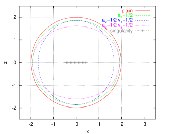
Figure 3: Apparent horizons for Kerr–Schild black holes with varying spins and boosts. Displayed is a cut through the $x$-$z$ plane.

VIII.2 Multiple black holes

In order to prepare and analyse initial data for binary black hole collision runs, I superposed two Kerr–Schild black holes as proposed in superposed-kerrschild , and then solved the constraint equations. This results in spacetimes with either two separate or a single distorted (“merged”) black holes. One can freely specify the locations, masses, and spins of the black holes prior to the superposition. The relation to the properties of the superposed black holes is not known, but it is hoped the superposition will not change them much.

For the superposition, I chose a grid spacing of $dx=1/4$, an outer boundary that has a distance $8.0$ from the centres of the black holes, and excised a spherical region with radius $1.0$ around the singularities. I superposed the three-metric and the extrinsic curvature without attenuation. I then solved the constraint equations using the York-Lichnerowicz method with a conformal transverse-traceless decomposition. (This method is described e.g. in livingreviews-cook , section 2.2.1.) I used Dirichlet boundary conditions for the vector potential and the conformal factor, keeping the boundary values from the superposition.

Whether or not a common apparent horizon exists is a hint as to whether the black hole configuration contains results from two separate or a single merged black holes; this fact is not known otherwise. The only way to find out would be to evolve this configuration for a long enough time so that the event horizon could be tracked backwards in time. This is unfortunately not easily possible (if at all) with today’s black hole evolution methods.

I created a series of initial data configurations for two equal-mass ($M=1$) non-spinning non-boosted black holes with varying distances. Table 5 shows the common horizons masses $M_{C}=R_{C}/2$, the individual horizons masses $M_{I}=R_{I}/2$, and the ADM masses of the spacetimes $M_{\mathrm{ADM}}$. The spins of the superposed black holes are known to be zero for symmetry reasons.

$z$	$R_{C}/2$	$R_{I}/2$	$M_{\mathrm{ADM}}$	$E_{B}$	$E_{R}$
0.0	2.280	—	2.306	—	+0.026
1.0	2.245	?	1.973	?	-0.272
1.75	2.167	1.137	1.986	-0.107	-0.181
2.0	2.130	1.087	1.989	-0.044	-0.141
2.5	2.023	1.041	1.994	-0.059	-0.029
3.0	(2.101)	1.020	1.997	(+0.060)	(-0.104)
4.0	—	1.002	2.000	-0.004
6.0	—	0.991	2.000	+0.018
8.0	—	0.989	2.000	+0.022

Table 5: Masses of the common horizons, the individual horizons, and the ADM masses for two superposed black holes for varying distances. $E_{B}$ is binding energy of the two black holes, and $E_{R}$ is amount of radiation present in the spacetime, as explained in the text. For $z=\pm 3.0$, no common horizon was detected any more. The last three rows show the sum of $E_{B}$ and $E_{R}$ only.

The row $z=0.0$ contains two black holes that were superposed at the same location, i.e. form a single black hole in a coordinate system different from Kerr–Schild. This is a consequence of the way the extrinsic curvatures are superposed. Note that the mass is not simply twice the mass of a single black hole. Also, as this spacetime is not spherically symmetric due to the outer boundary condition, the ADM mass and the horizon mass need not be the same.

In the row $z=\pm 3.0$, the apparent horizon finder did not converge, but was close. The $L_{2}$-norm of the residual was still $0.0248$ when the solver aborted. That means that from this row on there is no common horizon any more, but the solution error here is still comparable to the discretisation error.

The difference $E_{B}=M_{C}-2M_{I}$ can be interpreted as the binding energy of the system. (Here $M_{C}=R_{C}/2$ and $M_{I}=R_{I}/2$ because the spin is zero.) The binding energy magnitude seems to decrease with distance, and is negative as it should be, except in the row $z=\pm 3.0$ where there was no common horizon detected any more.

The difference $E_{R}=M_{\mathrm{ADM}}-M_{C}$ is the amount of radiation present in the spacetime. Of course, $E_{R}$ must be positive, meaning that the negative values found numerically are unphysical and point to numerical errors. I suspect that the error lies mainly with the calculation of the ADM mass. I calculate the ADM mass as a surface integral near the outer boundary. When I evaluate the integral at locations further inwards, closer to the apparent horizon, then the ADM mass increases and gets closer to the horizon mass. This is inconsistent and cannot happen when the constraints are satisfied. However, in a numerically given spacetime the constraints are only satisfied up to the discretisation error. It is thus in my opinion a bad idea to calculate the ADM mass (which is a global quantity) from information near the outer boundary only, relying on the constraints to propagate the necessary information to the boundary. A better method to calculate the ADM mass is needed. I decided to present the ADM values here nonetheless, because they (although inaccurate) still provide some insight into the spacetimes.

Figure 4 shows the apparent horizons of two superposed black holes with centres at $z=\pm 2.0$. The common apparent horizon indicates that there is a common event horizon present, and that this time slice thus contains a single, merged black hole. In figure 5, the black holes are closer together at $z=\pm 1.75$. The two inner apparent horizons actually do overlap; this is not a numerical error. It is surprising to see that the shape of the horizons is not distorted more. But unlike event horizons, there is no reason why apparent horizons should deform or join when two black holes approach each other.

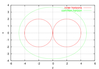
Figure 4: Common and individual horizons for superposed Kerr–Schild data at $z=\pm 2.0$.

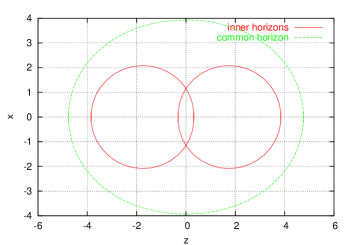
Figure 5: Common and individual horizons for superposed Kerr–Schild data at $z=\pm 1.75$. The individual horizons do overlap, and are surprisingly only minimally distorted.

Figure 6 shows the the common apparent horizons for a series of black holes with increasing distances. As the black holes are placed further apart, the common horizons become unsurprisingly more elongated. Figure 7 shows both the individual and common black holes for varying distances for comparison. Near $z=\pm 3.0$, the common horizon ceases to exist.

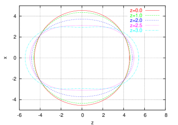
Figure 6: Common horizons for a series of merged black holes with increasing distances.

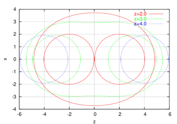
Figure 7: Individual and common horizons for superposed Kerr–Schild black holes near $z=\pm 3.0$, where the common apparent horizon disappears.

IX Summary

Apparent horizons provide valuable insight into spacetimes, such as mass and spin estimates for black holes. They are indicators for event horizons, and help keep track of the location of singularities. They provide necessary information for the time evolution of black hole spacetimes. This apparent horizon finding algorithm provides a fast way to track horizons during a numerical evolution, and also a robust way to find horizons in initial data, or as they appear during an evolution.

References

- [1] M. Alcubierre, S. Brandt, B. Bruegmann, C. Gundlach, J. Massó, E. Seidel, and P. Walker. Test-beds and applications for apparent horizon finders in numerical relativity. Class. Quant. Grav., 17:2159–2190, 2000.
- [2] P. Anninos, K. Camarda, J. Libson, J. Massó, E. Seidel, and W.-M. Suen. Finding apparent horizons in dynamic 3d numerical spacetimes. Phys. Rev. D, 58:024003, 1998.
- [3] Abhay Ashtekar, Christopher Beetle, and Olaf Dreyer. Generic isolated horizons and their applications. Phys. Rev. Lett., 85:3564–3567, 2000.
- [4] Abhay Ashtekar, Christopher Beetle, and Jerzy Lewandowski. Mechanics of rotating isolated horizons. Phys. Rev. D, 64:044016, 2001.
- [5] Cactus Authors. Cactus home page. http://www.cactuscode.org/, 2002.
- [6] Satish Balay, William D. Gropp, Lois C. MacInnes, and Barry F. Smith. PETSc home page. http://www.mcs.anl.gov/petsc, 1998.
- [7] Satish Balay, William D. Gropp, Lois C. McInnes, and Barry F. Smith. PETSc users manual. Technical Report ANL-95/11 - Revision 2.1.0, Argonne National Laboratory, 2000.
- [8] Thomas W. Baumgarte, Gregory B. Cook, Mark A. Scheel, Stuart L. Shapiro, and Saul A. Teukolsky. Implementing an apparent-horizon finder in three dimensions. Phys. Rev. D, 54:4849–4857, 1996.
- [9] Gregory B. Cook. Initial data for numerical relativity. Living Reviews in Relativity, 3(5), 2000.
- [10] Carsten Gundlach. Pseudo-spectral apparent horizon finders: an efficient new algorithm. Phys. Rev. D, 57:863–875, 1998.
- [11] Mijan F. Huq, Matthew W. Choptuik, and Richard A. Matzner. Locating boosted Kerr and Schwarzschild apparent horizons. gr-qc/0002076, submitted to Phys. Rev. D, 2000.
- [12] Richard A. Mazner, Mijan F. Huq, and Deirdre Shoemaker. Initial data and coordinates for multiple black hole systems. Phys. Rev. D, 59:024015, 1999.
- [13] Eberhard Pasch. The level set method for the mean curvature flow on (R3,g). Technical Report 63, SFB 382, SFB 382–Geschäftsstelle, Auf der Morgenstelle 10, 72076 Tübingen, Germany; Web: http://www.uni-tuebingen.de/uni/opx/projekte.html, 1997.
- [14] Deirdre M. Shoemaker, Mijan F. Huq, and Richard A. Matzner. Generic tracking of multiple apparent horizons with level flow. Phys. Rev. D, 62:124005, 2000.
- [15] Jonathan Thornburg. Numerical Relativity in Black Hole Spacetimes. PhD thesis, University of British Columbia, 3 1993.
- [16] Jonathan Thornburg. Finding apparent horizons in numerical relativity. Phys. Rev. D, 54:4899–4918, 1996.
- [17] Steven Weinberg. Gravitation and Cosmology, chapter 6.6, page 165 ff. John Wiley and Sons, 1972.