Static Negative Energies Near a Domain Wall

Abstract

We show that a system of a domain wall coupled to a scalar field has static negative energy density at certain distances from the domain wall. This system provides a simple, explicit example of violation of the averaged weak energy condition and the quantum inequalities by interacting quantum fields. Unlike idealized systems with boundary conditions or external background fields, this calculation is implemented precisely in renormalized quantum field theory with the energy necessary to support the background field included self-consistently.

Introduction

In the absence of any restriction on the matter stress-energy tensor $T^{\mu\nu}$, general relativity permits the construction of arbitrary spacetime geometries. One simply writes down the desired geometry and solves Einstein’s equation in reverse to determine $T^{\mu\nu}$. Thus it appears that the feasibility of producing exotic situations such as closed timelike curves (however see Krasnikov (2001, 2002)) and superluminal travel depends on whether energy conditions restrict $T^{\mu\nu}$. In particular, if one assumes the weak energy condition, $T_{\mu\nu}V^{\mu}V^{\nu}\geq 0$ for all timelike vectors $V^{\mu}$, or equivalently that no observer sees negative energy density, then one can show that superluminal travel Olum (1998) and the construction of closed timelike curves Tipler (1976, 1977); Hawking (1992) are impossible.

The weak energy condition is obeyed by the usual classical fields, but quantum fields can violate it. Perhaps the simplest example of weak energy condition violation is a superposition of the vacuum and a single mode with 2 photons. The negative energy densities are confined to particular regions of space and particular periods of time. In this system, and in any system made from free fields Klinkhammer (1991), the energy density satisfies the averaged weak energy condition,

$$\int_{\cal G}T_{\mu\nu}V^{\mu}V^{\nu}\geq 0\,,$$ (1)

where the integral is taken over a complete timelike geodesic ${\cal G}$ with tangent vector $V^{\mu}$. This energy density also satisfies quantum inequalities Ford and Roman (1997) of the form

$$\int\rho({\bf x},t)W(t)dt\geq-ct_{0}^{-d}$$ (2)

where $\rho=T_{00}$, $W$ is a window function of width $t_{0}$, $d$ is the number of spacetime dimensions, and $c$ is a constant depending on $d$, the type of field being considered, and the particular shape of $W$.

On the other hand, the best-known system exhibiting negative energy density is the Casimir problem. Casimir Casimir (1948) computed the energy density of the quantum electromagnetic vacuum between perfectly conducting plates separated by a distance $d$ and found

$$\rho=-\frac{\pi^{2}}{720d^{4}}\,.$$ (3)

Laboratory measurements Bressi et al. (2002) of the force associated with this energy have found good agreement with Casimir’s result. While a question has been raised Helfer and Lang (1999) whether the energy density between metal plates (as opposed to idealized perfect conductors) is actually negative, it does appear to be so Sopova and Ford (2002) as long as the separation of the plates is large enough. Since the negative energy density in the Casimir effect is static, it can be averaged for arbitrarily long times. Thus the Casimir effect violates the averaged weak energy condition and the quantum inequalities.

One way to think of the Casimir effect is as the energy of the electromagnetic vacuum with specified boundary conditions or with interaction with fixed materials. In that model, the electromagnetic field energy is subject to “difference quantum inequalities” Ford and Roman (1995), which restrict the energy density to be not much more negative than that in the vacuum with the specified conditions. However, one can also think of the Casimir effect as the energy of a system of coupled fields, including both the electromagnetic field and the fields of the matter that makes up the plates. In that case, the Casimir system is just a particular excitation of some interacting quantum fields above the vacuum. It contains static negative energy densities and is not restricted by any quantum inequality, because those apply only to free fields.

Unfortunately, the actual Casimir system is quite complicated, and to be certain to understand it one must take into account many effects associated with physical metals, such as the true dispersion relation and surface roughness. This letter demonstrates the same phenomenon of static negative energy density in a simpler system, consisting only of two scalar fields in 2+1 dimensions. Negative energies have appeared previously in calculations of quantum energy densities (see for example Bordag and Lindig (1996)); our emphasis here is that the complete energy density, including the energy required to support the background field, is negative in a self-consistent approximation with definite renormalization conditions.

Model

In order to have a system of scalar fields that is static and does not dissipate, we will use a topological defect. For simplicity of calculation and similarity to the Casimir problem we will use a domain wall, and to decrease the number of divergences requiring renormalization we will work in 2+1 dimensions. We thus define a real scalar field $\chi$ to form the domain wall and a second real scalar field $\phi$ whose interactions with $\chi$ will produce the negative energy density. The Lagrangian is

$${\cal L}=\frac{1}{2}\left[\partial_{\mu}\chi\partial^{\mu}\chi+\partial_{\mu}\phi\partial^{\mu}\phi+U(\chi,\phi)\right]$$ (4)

with

$$U(\chi,\phi)=\lambda(\chi^{2}-\eta^{2})^{2}+m^{2}\ (1-\chi^{2}/\eta^{2})\phi^{2}+\beta\phi^{4}\,.$$ (5)

With $\beta>m^{4}/(4\lambda\eta^{4})$ we find that $U$ is positive definite, and the classical ground state is given by $\phi=0$ and $\chi=\eta$ or $\chi=-\eta$. If we specify different vacua for $x\to\infty$ and $x\to-\infty$, we find a static classical domain wall solution. Taking the wall to lie on the $y$ axis, we find

$$\chi(x)=\eta\tanh(x/a)$$ (6)

where $a=1/(\sqrt{\lambda}\eta)$. The wall is invariant under translations and boosts in the $y$ direction. It has classical energy density

$$\rho(x)=2\lambda\eta^{4}\mathop{\rm sech}\nolimits^{4}(x/a)\,.$$ (7)

Now we quantize our fields. If we work in the regime where $m\ll\sqrt{\lambda}\eta$, the back reaction due to the quantized $\phi$ will have a negligible effect on the domain wall. We can thus consider the domain wall, for the purposes of the calculation, to provide a fixed background potential for $\phi$. The effective Lagrangian is then

$${\cal L}_{\phi}=\frac{1}{2}\left[\partial_{\mu}\phi\partial^{\mu}\phi-V(x)\phi^{2}\right]$$ (8)

where the potential

$$V(x)=m^{2}(1-\chi^{2}/\eta^{2})=m^{2}\mathop{\rm sech}\nolimits^{2}(x/a)$$ (9)

acts as a position-dependent mass term for $\phi$. Quantizing $\chi$ produces a correction to the shape of the domain wall and to its energy, but the energy density still falls exponentially as one goes away from the center of the wall. The change of shape will affect the Casimir energy associated with $\phi$, but only at higher order, which we will not consider here Bashinsky (2000).

A simple argument

We would like to show that a negative energy density exists somewhere. The energy density in the background potential can be calculated exactly, and we will do so below, but a detailed calculation is not necessary to demonstrate the existence of negative energy densities.

Suppose that instead of the background potential we had a perfectly reflecting boundary at $x=0$, i.e., $\phi(0)=0$. Then the computation would be straightforward and the energy density at $x$ would be

$$\rho_{\phi}(x)=-\frac{1}{32\pi x^{3}}$$ (10)

In this computation the main contribution to the energy density at $x$ comes from those modes whose wavelength $\lambda$ is similar to $x$. If we take $x$ sufficiently large, then we will be interested in large $\lambda$, and for sufficiently large $\lambda$, any potential barrier is perfectly reflecting Therefore, for sufficiently large $x$, the energy in $\phi$ approaches the form of Eq. (10). To this energy we must add the energy of the $\chi$ field, given in the classical approximation by Eq. (7), from which

$$\rho_{\chi}(x)\sim e^{-4|x|/a}\,.$$ (11)

Even if we take into account quantum corrections to the domain wall profile, we still expect $\rho_{\chi}$ to decline exponentially away from the wall because $\chi$ is a massive field.

Thus the positive energy density associated with the wall declines exponentially, while the negative energy density associated with $\phi$ declines only as a power law. For large enough $x$, the negative energy will dominate, and the total energy will approach the form of Eq. (10).

Calculation

The general calculation of the Casimir energy density for a scalar field with a background potential will be presented elsewhere Graham and Olum (2002). The energy density can be computed from the Green’s function for the given potential in scattering theory,

$$\rho(x)=-{1\over 8\pi}\int_{0}^{\infty}d\kappa\left[2\kappa^{3}G(x,x,i\kappa)-\kappa^{2}+\frac{V(x)}{2}-\kappa\frac{d^{2}}{dx^{2}}G(x,x,i\kappa)\right]$$ (12)

where $G(x,x^{\prime},k)$ is the Green’s function that satisfies

$$-G^{\prime\prime}(x,x^{\prime},k)+V(x)G(x,x^{\prime},k)-k^{2}G(x,x^{\prime},k)=\delta(x-x^{\prime})$$ (13)

and has only outgoing waves ($\sim e^{ik|x|}$) at infinity.

The problem of the potential of Eq. (9) can be solved exactly. The normal modes are associated Legendre functions and the Green’s function is

$$G(x,x^{\prime},k)=\frac{a}{2}\Gamma(1+s-ika)\Gamma(-s-ika){\rm P}^{ika}_{s}(\tanh(x_{>}/a)){\rm P}^{ika}_{s}(-\tanh(x_{<}/a))$$ (14)

where $x_{<}$ and $x_{>}$ are respectively the smaller and the larger of $x$ and $x^{\prime}$, ${\rm P}^{\mu}_{\nu}(x)$ is the associated Legendre function defined as in Bateman manuscript project (1953) for $-1<x<1$, and $s=(\sqrt{1-4m^{2}a^{2}}-1)/2$. We have

$$G(x,x,i\kappa)=\frac{a}{2}\Gamma(1+s+\kappa a)\Gamma(-s+\kappa a){\rm P}^{-\kappa a}_{s}(\tanh(x/a)){\rm P}^{-\kappa a}_{s}(-\tanh(x/a))\,.$$ (15)

If we put Eq. (15) into Eq. (12) and introduce the dimensionless variables $q=\kappa a$ and $y=x/a$ and the parameter $v=m^{2}a^{2}$, we get

$$-\frac{1}{8\pi a^{3}}\int_{0}^{\infty}dq\bigg{[} \Gamma(1+s+q)\Gamma(-s+q)\left(q^{3}-\frac{q}{2}\frac{d^{2}}{dy^{2}}\right)\left({\rm P}^{-q}_{s}(\tanh y){\rm P}^{-q}_{s}(-\tanh y)\right)$$ (17)

$$-q^{2}+{v\over 2}\mathop{\rm sech}\nolimits^{2}y\bigg{]}$$

We are concerned with the regime where $m$ is small compared to the inverse width of the wall, $1/a$, so $v\ll 1$. Fig. 1 shows the energy density in the case where $v=0.1$. For $y\gtrsim 3$, the energy density is negative, as predicted above.

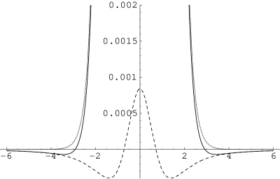
Figure 1: Energy density in the wall (dotted) and the field $\phi$ (dashed) and the total energy density (solid) in units where $\eta=1$ for parameters $\lambda=1$ and $m^{2}=0.1$. For sufficiently large values of $x$, the total energy density is negative.

Discussion

We have shown a specific example of two interacting scalar fields whose energy density is static and negative in certain regions. Since the system is static, one can average over as much time as one chooses, and thus the system violates the averaged weak energy condition and the quantum inequalities. From this system (as from the Casimir effect with physical plates) one sees that the averaged weak energy condition and the quantum inequalities are simply not correct in the case of interacting fields, so the failure of attempts to prove them is not due merely to technical reasons.

The present system does, however, satisfy the averaged null energy condition, given by Eq. (1) with $V^{\mu}$ null, which is sufficient to rule out superluminal travel and the construction of time machines. It is obeyed because if the geodesic runs parallel to the domain wall, then the positive pressure cancels the negative energy density and $T_{\mu\nu}V^{\mu}V^{\nu}=0$, while if the geodesic is not parallel to the wall it must cross through the region of high positive energy. It is not clear at this point whether some similar arrangement, such as a domain wall in 3+1 dimensions with a hole, might violate the averaged null energy condition for certain geodesics.

References

- Krasnikov (2001) S. Krasnikov (2001), eprint [http://arXiv.org/abs]gr-qc/0111054.
- Krasnikov (2002) S. Krasnikov, Phys. Rev. D65, 064013 (2002), eprint [http://arXiv.org/abs]gr-qc/0109029.
- Olum (1998) K. D. Olum, Phys. Rev. Lett. 81, 3567 (1998), eprint [http://arXiv.org/abs]gr-qc/9805003.
- Tipler (1976) F. J. Tipler, Phys. Rev. Lett. 37, 879 (1976).
- Tipler (1977) F. J. Tipler, Ann. Phys. (NY) 108, 1 (1977).
- Hawking (1992) S. W. Hawking, Phys. Rev. D 46, 603 (1992).
- Bekenstein (1974) J. D. Bekenstein, Ann. Phys. 82, 535 (1974).
- Klinkhammer (1991) G. Klinkhammer, Phys. Rev. D 43, 2542 (1991).
- Ford and Roman (1997) L. H. Ford and T. A. Roman, Phys. Rev. D 55, 2082 (1997), gr-qc/9607003.
- Casimir (1948) H. B. G. Casimir, Proc. Kon. Ned. Akad. Wet. B51, 793 (1948).
- Bressi et al. (2002) G. Bressi, G. Carugno, R. Onofrio, and G. Ruoso (2002), eprint [http://arXiv.org/abs]quant-ph/0203002.
- Helfer and Lang (1999) A. D. Helfer and A. S. I. D. Lang, J. Phys. A32, 1937 (1999), eprint [http://arXiv.org/abs]hep-th/9810131.
- Sopova and Ford (2002) V. Sopova and L. H. Ford (2002), eprint [http://arXiv.org/abs]quant-ph/0204125.
- Ford and Roman (1995) L. H. Ford and T. A. Roman, Phys. Rev. D 51, 4277 (1995), gr-qc/9410043.
- Bordag and Lindig (1996) M. Bordag and J. Lindig, J. Phys. A29, 4481 (1996).
- Bashinsky (2000) S. V. Bashinsky, Phys. Rev. D 61, 105003 (2000), hep-th/9910165.
- Barton (1985) G. Barton, J. Phys. A 18, 479 (1985).
- Graham and Jaffe (1999) N. Graham and R. L. Jaffe, Nucl. Phys. B 544, 432 (1999), hep-th/9808140.
- Graham and Olum (2002) N. Graham and K. D. Olum, Negative energies in quantum field theory with a background potential (2002), eprint [http://arXiv.org/abs]hep-th/0211244.
- Bateman manuscript project (1953) Bateman manuscript project, Higher transcendental functions, vol. 1 (McGraw-Hill, New York, 1953).