Reconcile Planck-scale discreteness
and the Lorentz-Fitzgerald contraction

Abstract

A Planck-scale minimal observable length appears in many approaches to quantum gravity. It is sometimes argued that this minimal length might conflict with Lorentz invariance, because a boosted observer could see the minimal length further Lorentz contracted. We show that this is not the case within loop quantum gravity. In loop quantum gravity the minimal length (more precisely, minimal area) does not appear as a fixed property of geometry, but rather as the minimal (nonzero) eigenvalue of a quantum observable. The boosted observer can see the same observable spectrum, with the same minimal area. What changes continuously in the boost transformation is not the value of the minimal length: it is the probability distribution of seeing one or the other of the discrete eigenvalues of the area. We discuss several difficulties associated with boosts and area measurement in quantum gravity. We compute the transformation of the area operator under a local boost, propose an explicit expression for the generator of local boosts and give the conditions under which its action is unitary.

]

I Introduction

A large number of convincing semiclassical considerations indicate that in a quantum theory of gravity the Planck length $L_{P}$ should play the role of minimal observable length [1]. Indeed, this happens, in different manners, in most, if not all, current tentative quantum gravity theories. It is often argued that the existence of this minimal length might signal a problem with Lorentz invariance (for instance, see [2]). A Lorentz invariant quantum theory can easily accommodate a basic observable length (in a free quantum field theory of a massive scalar field, for instance, there is the Compton wavelength of the particle), but is a minimal observable length compatible with some form of Lorentz invariance? One might argue that length transforms continuously under a Lorentz transformation, and a minimal length $L_{P}$ is going to get Lorentz contracted in a boost. Thus, a boosted observer should see a Lorentz contracted $L_{P}$, namely a length shorter than the length claimed to be minimal, leading to a contradiction.

This arguments is certainly simple minded, but it has had large resonance on quantum gravity research. The apparent conflict between Lorentz transformations and Planck scale discreteness, for instance, is often quoted as one of the motivations for quantum deformations of the Lorentz symmetry, and the use of quantum groups, or q-deformed Lorentz algebras, in this context. Within canonical quantum gravity, similar arguments have been used to suggest that no state of the theory can be locally Lorentz invariant, and so on.

In any case, it is clear that an approach to quantum gravity predicting that an observer ${\cal O}$ observes a minimal length $L_{P}$ must answer the question whether or not a boosted observer ${\cal O}^{\prime}$ can observe this length Lorentz contracted. And whether or not, in this sense, Planck scale discreteness can be compatible with some form of local Lorentz invariance.

Here, we show how the apparent conflict between Lorentz contraction and Planck scale discreteness is resolved in loop quantum gravity [3] (for a review and extended references, see [4] and [5].) Within loop quantum gravity, a minimal length appears characteristically in the form of a minimal (nonzero) value $A_{0}$ of the area of a surface [6, 7]. Here we show that in loop quantum gravity a boosted observer ${\cal O}^{\prime}$ does not observe a Lorentz contracted $A_{0}$. The minimal (nonzero) area that the boosted observer ${\cal O}^{\prime}$ can observe is still $A_{0}$. We show that Planck scale discreteness is compatible with a certain implementation of local Lorentz invariance, and we study the transformation properties of the area operator under an infinitesimal local boost.

A The basic idea

The key to understand how this may happen is the fact that in loop quantum gravity a minimal length does not appear as a fixed structural property of space geometry. Space geometry, indeed, has no fixed structural property at all in this approach. The geometry of space comes from a quantum field, the quantum gravitational field. Therefore the observable properties of the geometry, such as, in particular, a length, or an area, are observable properties of a quantum physical system. A measurement of a length is therefore a measurement in the quantum mechanical sense. Generically, quantum theory does not predict an observable value: it predicts a probability distributions of possible values. Given a surface moving in spacetime, the two measurements of its area performed by two observers ${\cal O}$ and ${\cal O}^{\prime}$ boosted with respect to each other are two distinct quantum measurements. Correspondingly, in the theory there are two distinct operators $A$ and $A^{\prime}$, associated to these two measurements. Now, our main point is the technical observation that $A$ and $A^{\prime}$ do not commute:

$$[A,A^{\prime}\,]\neq 0.$$ (1)

This is because $A$ and $A^{\prime}$ depend on the gravitational field on two distinct 2d surfaces in spacetime (see Figure 1) and a field operator does not commute with itself at different times. In this paper, we prove equation (1).

FIG. 1.: Two observers in relative motion (arrows) see two different table’s 2d surfaces (ovals) in spacetime, because their simultaneity surfaces are different and have thus a different intersection with the table worldsheet (cylinder).

It follows that a generic eigenstate of $A$ is not an eigenstate of $A^{\prime}$. If the observer ${\cal O}$ measures the area and obtains the minimal value $A_{0}$, the state of the gravitational field will be projected on an eigenstate of $A$. This, in turn, is not going to be an eigenstate of $A^{\prime}$. If then the observer ${\cal O}^{\prime}$ measures the area, he will therefore find the state in a superposition of eigenstates of $A^{\prime}$. That is to say, the theory predicts that, for him, the surface does not have a sharp area. If the experiment is repeated several times, ${\cal O}^{\prime}$ will observe a probability distribution of area values. The mean value of the area can be Lorentz contracted, while the minimal nonzero value of the area can remain $A_{0}$.

The situation is analogous to what happens with angular momentum in the ordinary quantum mechanics of a rotationally invariant system with given (say half-integer) spin. Consider a certain direction, say the $z$ direction. If we measure the component $L_{z}$ of the angular momentum, we have a discrete spectrum with a minimal nonzero value $L_{0}$. One might argue that this prediction conflicts with rotation invariance: if classical angular momentum components change continuously under a rotation – how can then an angular momentum component have a minimal value? But of course this concern is ill founded. If an observer ${\cal O}^{\prime}$ rotated with respect to $\cal O$ observes his own angular momentum component $L_{z}^{\prime}$, he will still observe the same minimal (nonzero) value $L_{0}$. In particular, if the observation follows the observation of the value $L_{0}$ by ${\cal O}$, and if the experiment is repeated, ${\cal O}$ will observe a distribution of eigenvalues which is uniquely determined by the well known representation theory of the rotation group in the Hilbert space of the theory. The same, we argue here, happens with the area in loop quantum gravity.

Although this analogy is very illuminating, however, the quantum gravity situation is far more complicated, for a number of reasons:

  i.

The theory as a whole is not Lorentz invariant, and a form of Lorentz invariance can only be recovered locally and/or in certain (“sufficiently flat”) regimes.

  ii.

The area $A$ is a far more complicated function of the basic variables of the theory than $L_{z}$.

  iii.

Lorentz transformations, unlike rotational symmetry, do not happen at fixed time. Therefore the generators of the (local) Lorentz transformations have to know about the dynamics of the theory, which is highly nontrivial in quantum gravity.

  iv.

The very construction of the “Lorentz rotated” quantity $A^{\prime}$ is delicate, since it involves a careful analysis in a general relativistic context of what it means to measure the area of a surface for a boosted observer.

  v.

The theory is invariant under diffeomorphisms; the area of a surface defined by coordinate values is not gauge invariant and we need a physical dynamical quantity to fix the surface whose area we want to consider [8].

For all these reasons, it is not obvious that the quantum area can behave “as the $L_{z}$ component of the angular momentum”. In this paper, we analyze all these problems with care, and we show that in spite of all these complications, and under certain reasonable assumptions, what happens to the area under a Lorentz boost in loop quantum gravity is indeed precisely what is described above and is illustrated by the analogy with the angular momentum.

Our strategy is the following. First, we address (v.) by considering a physical system formed by general relativity coupled to a minimal and realistic amount of matter, sufficient to have a well defined and diffeomorphism invariant notion of area. Notice that this is precisely the context in which the claim that the discretization of the area is a physically observable prediction of the theory was put forward [9]. Second, we address (iv.) by carefully discussing the meaning of the measurement of the area $A^{\prime}$ “seen” by a boosted observer in classical general relativity (Section II.) Then, we solve (ii.) by explicitly computing $A$ and $A^{\prime}$ as functions of the canonical variables of the theory (Section III.) This is done in a power expansion in the boost parameter, which allows us to address (iii.) by expressing quantities at $t>0$ in terms of quantities at $t=0$, using the equations of motion. In turn, this result allows us to derive (1) and compute explicitly the first terms of this commutator in an expansion in the boost parameter (Section IV.) Then (Section V), we construct a quantity that we suggest could generate the boost. This generator depends on the hamiltonian constraints, thus addressing (iii.). Finally in Section V A we derive the conditions under which this transformation is unitary, and thus the spectrum preserved.

Finally, (i.) is addressed by means of a delicate interplay between the full dynamical structure of the theory and the request of local flatness needed to have Lorentz invariance over a small spacetime region. We are interested in small scale quantum discreteness and small scale quantum fluctuations of the gravitational field, in quantum states in which the metric is macroscopically flat. That is, in which the macroscopic expectation value of the metric operator, is flat. To describe this regime, we first analyze the problem in the classical theory: we expand for small boost parameter and small surface, and keep only the lowest order relevant terms. We then assume that in the quantum theory the expansion remains valid in the regimes where the expectation value of the macroscopic curvature is small. This is not different from what we usually do in conventional quantum field theory: we take the field to be zero in the vacuum and expand around this value – even if the field fluctuates widely on small scale, and its value is moved far away from zero by a field measurement at small scale. Of course in nonperturbative quantum gravity we have far less control on the quantum state of the gravitational field that corresponds to macroscopical flat space, and therefore the viability of this approach we should cautionally be regarded as an hypothesis.

In addition, in Section IV A we briefly discuss an alternative point of view, which we have learned in conversations with Amelino-Camelia, on the non commutativity between $A$ and $A^{\prime}$. The idea is to view the non commutativity of $A$ and $A^{\prime}$ as a consequence of the noncommutativity between the area of the surface and the relative velocity of the observer and the surface. We refer to [10] for a more extensive discussion.

II Geometry

A The system

We consider the physical system formed by four physical elements:

  i.

the gravitational field,

  ii.

two particles,

  iii.

a two-dimensional surface (the “table”).

These are the dynamical quantities of the system we consider. They provide a minimal setting in which we can compare the area observed by two observers boosted with respect each other. We are interested in the area of the table, as seen by two observers (${\cal O}$ and ${\cal O}^{\prime}$), moving with the two particles.

Besides these dynamical quantities, we assume that all sort of other physical objects exist in the universe. These can be used to perform measurements (for instance, light pulses traveling along geodesics, apparatus that detect the arrival of these light pulses, clocks that measure proper time along world lines, recording devices and so on). We do not consider these other physical objects as part of the dynamical system observed: we consider them as part of the measuring apparatus. To be precise, we assume that the well known freedom of choosing the boundary between the observed quantum system and the classical apparatus –emphasized by Von Neumann– allows us to do so in this context.

We describe the system in a general relativistic setting as follows. We consider a 4d manifold $\cal M$, with coordinates $x^{\mu}$, on which the following quantities are defined:

  i.

The gravitational field $g$ is described by the metric tensor $g_{\mu\nu}(x)$.

  ii.

The world lines $X$ and $X^{\prime}$ of the two observers are given by the functions

$$X : R\to{\cal M}$$ (2)

$$: \tau\mapsto x^{\mu}(\tau)$$ (3)

and

$$X^{\prime} : R\to{\cal M}$$ (4)

$$: \tau^{\prime}\mapsto x^{\mu}(\tau^{\prime})$$ (5)

(we follow here the bad physicists’ habit of indicating functions with the name of the independent and dependent variable: $x^{\mu}(\tau^{\prime})$ is given by a different function that $x^{\mu}(\tau)$, of course.)

  iii.

The world sheet $T$ of the table is described by the three-dimensional hypersurface

$$T : [-1,+1]\times[-1,+1]\times R\to{\cal M}$$ (6)

$$: (\tau^{1},\tau^{2},\tau^{3})\mapsto x^{\mu}(\tau^{1},\tau^{2},\tau^{3})$$ (7)

The functions $(g_{\mu\nu}(x),\ x^{\mu}(\tau),\ x^{\mu}(\tau^{\prime}),\ x^{\mu}(\tau^{1},\tau^{2},\tau^{3}))$ are the lagrangian variables of the system. We assume the dynamics of this system to be governed by the the Einstein equations and the dynamical equations of the table and the particles. For simplicity, we assume that the matter energy-momentum tensor is negligible in the Einstein equations, but this is not essential in what follows.

We are interested in a specific subset of physical configurations. First, we want the world lines of the two observers to cross at a point $P$ situated on the table world sheet. Second, (in the classical analysis) we assume that the curvature at and around $P$ and the acceleration of the particles at $P$ are negligible at the scale of the surface. That is, we take the surface small enough that we can expand around $P$ and keep the lowest terms only.

What is the area $A$ of the table seen by $\cal O$ when at $P$? The answer is the following. $A$ is the area of the 2d surface $S$ formed by the intersection of the 3d table’s worldsheet $T$ with the 3d simultaneity surface $\Sigma$ of $\cal O$ at $P$.

FIG. 2.: The definition of the simultaneity surface.

The simultaneity surface $\Sigma$ is the set of points in $\cal M$ whose light cone intersects $X$ in two points at the same proper time distance (along $X$) from $P$. Physically, these are the events where a mirror reflects a light pulse emitted by the observer at proper time $-t$ such that the reflected pulse gets back to the observer at proper time $+t$ ($t=0$ being at $P$). This is Einstein definition of (relative) simultaneity. (See Figure 2.)

The intersection between the surface of simultaneity of the observer $\Sigma$ and the table world history $T$ is a two dimensional surface $S=\Sigma\cap T$. It represents the “table at fixed time” in the frame of the observer $\cal O$ at $P$. The area $A$ is the integral over $S$ of the determinant of the restriction ${}^{2}g$ of the metric $g$ to $S$. The area $A$ is therefore a complicated function $A[g,X,X^{\prime},T]$ of —but it is completely determined by— the metric $g$ the world line $X$, the hypersurface $T$, and the crossing point $P$. We calculate this function explicitly in Section II B. Similarly, $A^{\prime}$ is the area of the intersection between $T$ and the simultaneity surface of ${\cal O}^{\prime}$ at $P$. (See Figure 3.)

We call $v^{\mu}$ (and, respectively, $v^{\prime}{}^{\mu}$) the unnormalized four-velocity of $X$ (respectively $X^{\prime}$) at $P$

$$v^{\mu}=\left.\frac{dx^{\mu}(\tau)}{d\tau}\right|_{P}.$$ (8)

($v^{\prime}{}^{\mu}$ is defined in the same manner by $x^{\mu}(\tau^{\prime})$.) The angle between the two tangents gives the relative speed $V$ of the two observers ${\cal O}$ and ${\cal O}^{\prime}$

$$\gamma=\frac{1}{\sqrt{1-V^{2}}}=\frac{v\cdot v^{\prime}{}}{|v|\,|v^{\prime}|}.$$ (9)

where the scalar product and the norm are taken here with the metric at $P$. For simplicity, we also assume that the relative three-velocity of the two observers is tangent to the table. (We are not interested in transversal motion because it does not give rise to Lorentz contraction.) We say that the table is at rest with respect to $X$, if the world sheet of the boundary of the table is normal to $\Sigma$. (If the surface is sufficiently small this implies that $A$ maximizes the area with respect to $v$.)

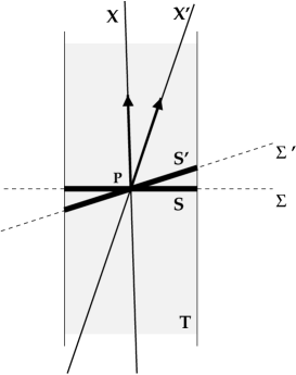
FIG. 3.: The definition of $S$ and $S^{\prime}$.

The quantities $A$ and $A^{\prime}$ are diffeomorphism invariant functions of $g$, $X$, $X^{\prime}$ an $T$. They are invariant under a smooth displacement of these dynamical quantities on $\cal M$. They do not depend on the coordinates chosen on $\cal M$, nor on any structure on $\cal M$ besides the dynamical fields. They are fully gauge invariant observables in this dynamical system. They are physical quantities that are in principle observable, by using appropriate measuring devices (formed by light pulses, detectors, clocks, and else). The specific technical construction of these devices is not relevant here.

In this paper we consider the quantum theory corresponding to this dynamical system. In particular, we consider the quantum operators corresponding to the physically observable quantities $A$ and $A^{\prime}$, we show that (1) is true, and that the operator $A^{\prime}$ can be obtained (under certain assumptions) from a unitary transformation that implements a local Lorentz transformation in the Hilbert space of the theory.

B Area in general relativity

What is the area $A(S)$ of the (small) 2d surface $S$ given by the intersection of two 3d hypersurfaces $\Sigma$ and $T$? Here we show that $A(S)$ can be written in terms of the one-forms $n_{\mu}^{\Sigma}$ and $n_{\mu}^{T}$ normal to the two hypersurfaces. We shall then use this fact to directly connect the area to the motion of the observers. The table worldsheet $T$ is parametrized by $x^{\mu}(\tau^{1},\tau^{2},\tau^{3})$. Its normal one-form is

$$n^{T}_{\mu}=\epsilon_{\nu\rho\sigma\mu}\ \frac{\partial x^{\nu}}{\partial\tau^{1}}\frac{\partial x^{\rho}}{\partial\tau^{2}}\frac{\partial x^{\sigma}}{\partial\tau^{3}}.$$ (10)

It does not depend on the metric. Similarly, the normal of the hypersurface $\Sigma$, parametrized as $x^{\mu}(\rho^{1},\rho^{2},\rho^{3})$, is

$$n^{\Sigma}_{\mu}=\epsilon_{\nu\rho\sigma\mu}\frac{\partial x^{\nu}}{\partial\rho^{1}}\frac{\partial x^{\rho}}{\partial\rho^{2}}\frac{\partial x^{\sigma}}{\partial\rho^{3}}.$$ (11)

The normal two-form of the intersection $S=\Sigma\cap T$ parametrized as $x^{\mu}(u,v)$, is

$$n_{\mu\nu}=\frac{1}{2}\epsilon_{\mu\nu\rho\sigma}\frac{\partial x^{\rho}}{\partial u}\frac{\partial x^{\sigma}}{\partial v}.$$ (12)

It is convenient to choose parametrizations such that

$$u= \tau^{1} =\rho^{1}$$ (13)

$$v= \tau^{2} =\rho^{2}$$ (14)

and

$$\epsilon_{\mu\nu\rho\sigma}\ \frac{\partial x^{\mu}}{\partial u}\frac{\partial x^{\nu}}{\partial v}\frac{\partial x^{\rho}}{\partial\tau^{3}}\frac{\partial x^{\sigma}}{\partial\rho^{3}}=1.$$ (15)

Then we have easily

$$n_{\mu\nu}=\ n^{\Sigma}_{[\mu}\ n^{T}_{\nu]}.$$ (16)

The area of a 2d surface is

$$A=A(S) = \int_{S}dudv\ \sqrt{\det{}^{2}g}$$ (17)

$$= \int_{S}dudv\ \sqrt{\det\left(\frac{\partial x^{\mu}}{\partial u^{i}}\frac{\partial x^{\nu}}{\partial u^{j}}\ g_{\mu\nu}\right)}.$$ (18)

where $u^{i}=(u,v)$ and the determinant is on the $i,j=1,2$ indices.

Consider now the equality

$$2gn_{\mu\nu}n_{\alpha\beta}g^{\mu\alpha}g^{\nu\beta} = \frac{g}{2}\epsilon_{\mu\nu\rho\sigma}\epsilon_{\alpha\beta\gamma\delta}\frac{\partial x^{\rho}}{\partial u}\frac{\partial x^{\sigma}}{\partial v}\frac{\partial x^{\gamma}}{\partial u}\frac{\partial x^{\delta}}{\partial v}g^{\mu\alpha}g^{\nu\beta}$$ (19)

$$= -\frac{1}{2}\epsilon_{\mu\nu\rho\sigma}\epsilon^{\mu\nu\zeta\theta}\frac{\partial x^{\rho}}{\partial u}\frac{\partial x^{\sigma}}{\partial v}\frac{\partial x_{\zeta}}{\partial u}\frac{\partial x_{\theta}}{\partial v}$$ (20)

$$= \frac{\partial x^{\rho}}{\partial u}\frac{\partial x_{\rho}}{\partial u}\frac{\partial x^{\sigma}}{\partial v}\frac{\partial x_{\sigma}}{\partial v}-\left(\frac{\partial x^{\rho}}{\partial u}\frac{\partial x_{\rho}}{\partial v}\right)^{2}$$ (21)

$$= \det\left(\frac{\partial x^{\mu}}{\partial u^{i}}\frac{\partial x^{\nu}}{\partial u^{j}}\ g_{\mu\nu}\right),$$ (22)

obtained using

$$\epsilon^{\alpha\beta\gamma\delta} = -g\epsilon_{\mu\nu\rho\sigma}g^{\mu\alpha}g^{\nu\beta}g^{\gamma\rho}g^{\delta\sigma},$$ (23)

$$\epsilon_{\mu\nu\rho\sigma}\epsilon^{\mu\nu\zeta\theta} = 2\ (\delta^{\zeta}_{\sigma}\delta^{\theta}_{\rho}-\delta^{\zeta}_{\rho}\delta^{\theta}_{\sigma}).$$ (24)

Using this, the area of $S$ can be written as ($g=\det\ g_{\mu\nu})$

$$A = \int_{S}dudv\ \sqrt{2\ g\ n_{\mu\nu}\ n_{\alpha\beta}\ g^{\mu\alpha}\ g^{\nu\beta}}$$ (25)

$$= \int_{S}dudv\ \sqrt{g\ (n^{T}_{\mu}n^{\Sigma}_{\nu}n^{T}_{\alpha}n^{\Sigma}_{\beta}-\ n^{T}_{\mu}n^{\Sigma}_{\nu}n^{\Sigma}_{\alpha}n^{T}_{\beta})\ g^{\mu\alpha}g^{\nu\beta}}$$ (26)

$$\equiv \int_{S}dudv\ \sqrt{g\ |n^{T}|^{2}\ |n^{\Sigma}|^{2}-(n^{T}\cdot n^{\Sigma})^{2}}$$ (27)

This expression gives us the area directly as a function of surface $S$, the metric and the normals to the table worldsheet and the observer’s simultaneity surface.

III Dynamics

A Coordinate choice

Without important loss of generality, we chose coordinates $x^{\mu}=(t,x^{1},x^{2},x^{3})$ which are particularly convenient for the above setting. In these preferred coordinates: (i) $P$ is the origin. (ii) The 3-surface $T$ is defined by $-1<x^{1}<+1$, $-1<x^{2}<+1$ and $x^{3}=0$. (iii) The world line $X$ is defined by $x^{1}=x^{2}=x^{3}=0$. (iv) The world line $X^{\prime}$ is defined by $x^{2}=x^{3}=0$ and $x^{1}=\beta x^{0}$. Furthermore we choose the parameters parametrizing the world lines and the world sheet as $\tau=\tau^{\prime}=\tau^{3}=t$, $u=\tau^{1}=x^{1}$ and $v=\tau^{2}=x^{2}$.

We also further fix the coordinates by choosing the gauge in which at $t=0$ we have $g_{00}=-1$ and $g_{a0}=0$ for $a=1,2,3$. This simplifies the canonical analysis.

A very important observation follows. With these coordinates, namely in this gauge, the only remaining degrees of freedom are the ones in the metric tensor $g_{\mu\nu}(x)$. However, this does not mean that the physical degrees of freedom of the matter (the two particles and the table) are being killed or frozen. Indeed, it is well known that the coordinate position of matter and the value of the metric tensor are both gauge dependent quantities, due to diffeomorphism invariance. The physical, measurable, position of an object (relative to a reference object) is determined by a combinations of the two.

Let us illustrate this key point in a simple one-dimensional universe with a metric field $g(x)$, an object $A$ in the coordinate positions $x=X$ and a reference object in the coordinate position $x=0$. The position of $A$ is determined by the distance from the reference

$$d[g,X]=\int_{0}^{X}dx\ \sqrt{g(x)}.$$ (28)

$d$ is a diffeomorphism invariant quantity. It corresponds to what we actually measure: pick a meter a get the position of $A$ in meters from the reference – this measures $d$. Now, we can gauge fix the coordinate $x$ so that $g=1$. In this gauge, the observable quantity $d$ is given by the coordinate position of the object:

$$d=X.$$ (29)

This is what we generally do in flat space: coordinates give observable positions. Alternatively, we can choose coordinates in which the position of the object has a fixed predetermined coordinate value $X=1$. In this gauge

$$d=\int_{0}^{1}dx\ \sqrt{g(x)}.$$ (30)

With this gauge choice, the physical location of the object, namely its distance $d$ from the reference is determined by the sole metric field.

These two possibilities are familiar, for instance, in the context of gravitational wave detectors: We can equivalently say that “the two mass probes do not move and the gravitational field varies in the in between region”; or that “the two mass probes oscillate in space” (where “move” and “oscillate” refer to the coordinates.) These are two equivalent descriptions of the same physics.

In the present context, we have chosen to attach coordinates to the matter (particles and table). Therefore the dynamics is entirely captured by the value of the gravitational field.

To further illustrate how the physical degrees of freedom of the table and the particle are still present, as well as for later purposes, consider for instance the following value of the metric, in the given coordinates:

$$ds^{2} = g_{\mu\nu}(x)\,dx^{\mu}dx^{\nu}$$ (31)

$$= -dt^{2}+(1+4\alpha x^{1}t)(dx^{1})^{2}+(dx^{2})^{2}+(dx^{3})^{2}.$$ (32)

Let $\vec{x}(t)$ be the trajectory of the central point of this table, that is, the point at the same distance from its boundaries. Easily, to first order in $t$,

$$\vec{x}(t)=\left(\alpha t,\ 0,\ 0\right).$$ (33)

Therefore the relative velocity of the particle $X$ with respect to the center of the table is $\alpha$. In other words, the particle $X$ and the table $T$ are moving with respect to each other even is their coordinate positions have been fixed. The relative velocity of table and particle is given by the time derivative of the metric field. ($g_{\mu\nu}(x)$ does not depend on $\alpha$ at $t=0$, while its time derivative does.) The example illustrate how the physical motion of the particles and table is described by components of the metric tensor in this gauge.

Now, since we have partially fixed the gauge by fixing the coordinate position of the matter, it follows that the invariance under general coordinate transformations is reduced to the invariance under the change of coordinates that preserve the coordinate condition chosen. Equivalently, the diffeomorphisms group Diff, which is the gauge group, is reduced in this gauge to the subgroup Diff₀ formed by the diffeomorphisms that send the table and particles’ worldlines into themselves.

As a consequence, certain components of the gravitational field that are gauge dependent quantities in pure general relativity, become gauge invariant physical quantities, precisely as the r.h.s. of (30). In particular, in this gauge the areas $A$ and $A^{\prime}$, which are gauge invariant observables, are expressed solely in terms of $g$, but they still remain, of course, gauge invariant.

We can clarify this point with an analogy from Maxwell theory: in the gauge in which scalar potential is set to zero, $A_{0}=0$, the electric field (a gauge invariant quantity) is given by the sole time derivative of the Maxwell vector potential: $\vec{E}=d\vec{A}/dt$. In this gauge $d\vec{A}/dt$ represents a gauge invariant quantity, because the gauge transformation are reduced to the ones that preserve $A_{0}=0$. Similarly, in the coordinates we have chosen the area is given by a function of $g$ alone, and is gauge invariant because it is invariant under coordinate transformations that preserve the coordinate choice made.

We have discussed these issues in great detail in this Section, because they are sources of frequent confusion. Let us now write $A$ explicitly as a function of the metric field in the coordinates we have chosen.

B Area as function of canonical coordinates

In the coordinates we have chosen, the table worldsheet $T$ is given by

$$T:\left\{\begin{array}[]{c}x^{3}=0,\\ -1<x^{1}<+1,\\ -1<x^{2}<+1\end{array}\right.$$ (37)

and the simultaneity surface $\Sigma$ of the first observer by

$$\Sigma: t=0.$$ (38)

Therefore

$$n^{\Sigma}_{\mu}=(-1,0,0,0),$$ (39)

$$n^{T}_{\mu}=(0,0,0,1).$$ (40)

Also, the proper time of the observer coincides with $t$. Equation (27) becomes the well known formula

$$A=A(S)=\int_{S}dudv\ \sqrt{\ \tilde{\tilde{g}}{}^{33}\ }.$$ (41)

where we have defined $\tilde{\tilde{g}}{}^{33}=(-\det g)\ g^{33}$. Explicitly, since $S$ is the intersection of the surface $\Sigma$ and the table worldsheet $T$ we have from (37) and (38)

$$A=\int_{-1}^{1}du\int_{-1}^{1}dv\ \sqrt{\ \tilde{\tilde{g}}{}^{33}(0,u,v,0)}.$$ (42)

Consider now the observer ${\cal O}^{\prime}$. His simultaneity surface $\Sigma^{\prime}$ is determined by the worldline $X^{\prime}$. The 4-velocity of this world line $X^{\prime}$ at $P$ is

$$v^{\prime}{}^{\mu}=(1,\ \beta,\ 0,\ 0).$$ (43)

If $g_{\mu\nu}$ is constant, $\Sigma^{\prime}$ is just normal to the 4-velocity (43): in the parametrization $\vec{\rho}=(\rho^{1},\rho^{2},\rho^{3})$ that we have chosen, it is given by

$$x^{\mu}(\vec{\rho})=(\beta\ g_{1a}\rho^{a},\vec{\rho})$$ (44)

where $a=1,2,3$. Using (11), we have, in the coordinates and parametrization chosen

$$n_{\mu}^{\Sigma^{\prime}}=(-1,\ \beta g_{1a}),$$ (45)

Since $g_{\mu\nu}(x)$ is in general not constant, the detailed calculation of the position of $\Sigma^{\prime}$ is more cumbersome. We can shortcut it, to linear order around $P$, by simply taking the value of $g_{\mu\nu}(x)$ in (44) at a point $\hat{x}^{\mu}=\frac{1}{2}x^{\mu}$ half way between $P$ and the point of the surface. (This is in “the middle” of path of the light that defines $\Sigma^{\prime}$. A more detailed calculation –which we do not report here– obtained integrating explicitly the light paths in a metric that grows linearly in time, confirms the result.) That is, to next order we replace (44) by

$$x^{\mu}(\vec{\rho})=\left(\beta g_{1a}(\hat{x}(\vec{\rho}))\,\rho^{a},\vec{\rho}\right).$$ (46)

This equation defines $x(\vec{\rho})$ intrinsically, since $x(\vec{\rho})$ appears in the r.h.s. as well. Explicitly, to second order in $\beta$ we have

$$x^{0}(\vec{\rho}) = \beta g_{1a}(0,\vec{\rho}/2)\rho^{a}+\frac{1}{2}\beta^{2}\dot{g}_{1b}(0,\vec{\rho}/2)\rho^{b}\ g_{1a}(0,\vec{\rho}/2)\rho^{a}\$$ (47)

$$x^{a}(\vec{\rho}) = \rho^{a}.$$ (48)

${\cal O}^{\prime}$’s simultaneity hypersurface defines the surface $S^{\beta}=\Sigma^{\prime}\cap T$, as the table seen by ${\cal O}^{\prime}$ at his fixed time. (See Figure 3.) Combining (48) and (37) we have, in the parametrization chosen, again to order $\beta^{2}$

$$x^{0}(u,v) = \beta g_{1i}(u/2,v/2)u^{i}$$ (50)

$$+\frac{\beta^{2}}{2}\dot{g}_{1i}(u/2,v/2)u^{i}g_{1j}(u/2,v/2)u^{j},$$

$$x^{1}(u,v) = u^{1}=u,$$ (51)

$$x^{2}(u,v) = u^{2}=v,$$ (52)

$$x^{3}(u,v) = 0.$$ (53)

Here and from now on, $g_{\mu\nu}(u,v)=g_{\mu\nu}(0,u,v,0)$ and $g_{\mu\nu}=g_{\mu\nu}(0,0,0,0)$

From (27) we have for the second observer

$$A^{\prime}=A(S^{\prime})=\int_{S^{\prime}}dudv\ \sqrt{\ \tilde{\tilde{g}}{}^{33}\ [1-\beta^{2}\,g_{11}]}.$$ (54)

Explicitly,

$$A^{\prime}=\int_{-1}^{1}\!\!\!\!du\!\int_{-1}^{1}\!\!\!\!dv\ \sqrt{\ \tilde{\tilde{g}}{}^{33}(x(u,v))\ [1-\beta^{2}\,g_{11}(x(u,v)]}.$$ (55)

Using (53), we have to order $\beta$

$$A^{\prime} = A+\frac{\beta}{2}\int_{-1}^{1}\!\!\!\!du\int_{-1}^{1}\!\!\!\!dv\ g_{1i}(u,v)\ u^{i}\$$ (57)

$$\ \ \ \ \ \ \ \ \ \times\ \ (\tilde{\tilde{g}}{}^{33}(u,v))^{-1/2}\ \dot{\tilde{\tilde{g}}}{}^{33}(u,v).$$

To order $\beta^{2}$ we have

$$A^{\prime}=\int_{-1}^{1}\!\!\!\!du\int_{-1}^{1}\!\!\!\!dv\ \sqrt{\ \tilde{\tilde{g}}{}^{33}(x(u,v))}$$ (58)

$$+\frac{\beta}{2}\int_{-1}^{1}\!\!\!\!du\int_{-1}^{1}\!\!\!\!dv\ \ g_{1i}(x(u,v))\ u^{i}\ (\tilde{\tilde{g}}{}^{33}(u,v))^{-\frac{1}{2}}\ \dot{\tilde{\tilde{g}}}{}^{33}(u,v)$$ (59)

$$+\frac{\beta^{2}}{4}\int_{-1}^{1}\!\!\!\!du\int_{-1}^{1}\!\!\!\!dv\ \ g_{1i}(u,v)u^{i}\ g_{1j}(u,v)u^{j}\$$ (60)

$$\ \ \ \ \ \ \ \ \ \times\ \ (\tilde{\tilde{g}}{}^{33}(u,v))^{-\frac{1}{2}}\ \ddot{\tilde{\tilde{g}}}{}^{33}(u,v)$$ (61)

$$-\frac{\beta^{2}}{8}\int_{-1}^{1}\!\!\!\!du\int_{-1}^{1}\!\!\!\!dv\ (\tilde{\tilde{g}}{}^{33}(u,v))^{-\frac{3}{2}}\ (g_{1i}(u,v)u^{i})^{2}(\dot{\tilde{\tilde{g}}}{}^{33})^{2}(u,v)$$ (62)

$$-\frac{\beta^{2}}{2}\int_{-1}^{1}\!\!\!\!du\int_{-1}^{1}\!\!\!\!dv\ g_{11}(u,v)\ (\tilde{\tilde{g}}{}^{33}(u,v))^{\frac{1}{2}},$$ (63)

and so on. The second, third and fourth line of this equation come from the time derivatives of $\tilde{\tilde{g}}{}^{33}$, which depend on $\beta$. The last line comes from the $\beta^{2}$ in (55). Notice that there is still a $\beta$ dependences in the first two lines, because $x(u,v)$, given in (53), contains $\beta$.

Let us now make the additional assumption that the metric is spatially constant at $t=0$. This simplifies the expressions above and allows us to perform the integrals explicitly, but it is not essential: it is easy to generalize our result to a non spatially constant metric. Under this condition we can write

$$g_{\mu\nu}(x(u,v)) = g_{\mu\nu}+\beta\ g_{1i}u^{i}\ \dot{g}_{\mu\nu}+\frac{\beta^{2}}{2}g_{1j}u^{j}\ \dot{g}_{1i}u^{i}\ \dot{g}_{\mu\nu}$$ (65)

$$+\frac{\beta^{2}}{2}g_{1j}u^{j}\ g_{1i}u^{i}\ \ddot{g}_{\mu\nu}.$$

Inserting this in the first two lines of (58), we can do all the integrals explicitly. The ones linear in $u$ vanish, leaving, to second order in $\beta$, with a straightforward calculation

$$A = \sqrt{\tilde{\tilde{g}}{}^{33}}$$ (66)

$$A^{\prime} = A-2\beta^{2}\ g_{11}A$$ (69)

$$+\beta^{2}\ (g_{11}^{2}+g_{22}^{2})\left(\frac{\partial^{2}_{t}\,\tilde{\tilde{g}}{}^{33}}{3A}-\frac{(\partial_{t}\,\tilde{\tilde{g}}{}^{33})^{2}}{6A^{3}}\right)$$

$$+\ \beta^{2}\ (g_{11}\dot{g}_{11}+g_{12}\dot{g}_{12})\ \frac{\partial_{t}\,\tilde{\tilde{g}}{}^{33}}{3A}.$$

IV Non commutativity

So far, we have simply studied the form of the areas $A$ and $A^{\prime}$ seen by two accelerated observers, in a given metric. Let us now recall that the metric is the gravitational field, namely a dynamical physical field. We want to write $A$ and $A^{\prime}$ as functions on the phase space of our dynamical theory, and compute the Poisson bracket $\{A,A^{\prime}\}$. To this aim, we take the simultaneity surface $\Sigma$, that is $t=0$ in the coordinates chosen, as our $ADM$ surface, on which we base the canonical formalism. As usual in quantum gravity, we chose as canonical variable the Ashtekar’s field $E^{a}_{i}(x)$, namely the densitized tetrad field, which satisfies

$$E^{a}_{i}(x)E^{b}_{i}(x)=\tilde{\tilde{g}}{}^{ab}(x).$$ (70)

We consider the metric field (which we leave indicated when convenient) as a function of the tetrad field. The explicit form of the brackets in the r.h.s. depends on the dynamics of the matter field, which in the coordinates we have chosen affects the dynamics of the gravitational field by partially constraining the evolution of Lapse and Shift. However, one can easily see that even if we assume that in these coordinates the dynamics of the gravitational field is unaffected by the matter, the r.h.s. does not vanish. In this case, indeed, we can take the evolution in the coordinate $t$ to be generated simply by the pure gravity hamiltonian constraint (we are in Lapse=1, Shift = 0 gauge), namely

$$\dot{E}_{i}^{a} = \{E^{a}_{i},H\},$$ (71)

$$\dot{A}_{a}^{i} = \{A^{i}_{a},H\},$$ (72)

where

$$H = \int d^{3}x\ E_{i}^{a}E_{j}^{b}F_{ab}^{k}\epsilon_{k}{}^{ij}$$ (73)

$$= \int d^{3}x\ E_{i}^{a}E_{j}^{b}\ (\partial_{a}A^{k}_{b}\epsilon_{k}{}^{ij}+A^{i}_{[a}A^{j}_{b]})).$$ (74)

Recalling that the non vanishing Poisson brackets are given by

$$\{E^{a}_{j}(x),A^{k}_{b}(y)\}=\delta^{a}_{b}\delta^{k}_{j}\ \delta^{3}(x,y),$$ (75)

we can compute the Poisson brackets explicitly.

Surprisingly,

$$\{\tilde{\tilde{g}}{}^{33},\dot{\tilde{\tilde{g}}}{}^{33}\}=0$$ (76)

and

$$\{\tilde{\tilde{g}}{}^{33},\ddot{\tilde{\tilde{g}}}{}^{33}\}=0.$$ (77)

The first equality follows from

$$\{\tilde{\tilde{g}}{}^{33},\dot{\tilde{\tilde{g}}}{}^{33}\} = 2E^{3}_{i}E^{3}_{j}\{E^{3}_{i},\dot{E}^{3}_{j}\}$$ (78)

$$= 2E^{3}_{i}E^{3}_{j}\{E^{3}_{i},E^{3}_{[j}E^{a}_{k]}A_{a}^{k}\}$$ (79)

$$= 2E^{3}_{i}E^{3}_{j}\ E^{3}_{[j}E^{3}_{i]}$$ (80)

$$= 0.$$ (81)

The second equality can be derived from

$$\{\tilde{\tilde{g}}{}^{33},\ddot{\tilde{\tilde{g}}}{}^{33}\}=E^{3}_{i}\{E^{3}_{i},(2\dot{E}^{3}_{j}\dot{E}^{3}_{j}+E^{3}_{j}\ddot{E}^{3}_{j})\}$$ (82)

Of the two terms on the r.h.s., the first is proportional to $\{E^{3}_{i},\dot{E}^{3}_{j}\}$, which, as he have just seen, vanishes. The second can be written as

$$E^{3}_{i}E^{3}_{j}\{E^{3}_{i},\ddot{E}^{3}_{j}\}=E^{3}_{i}E^{3}_{j}(\partial_{t}\{E^{3}_{i},\dot{E}^{3}_{j}\}-\{\dot{E}^{3}_{i},\dot{E}^{3}_{j}\});$$ (83)

again, the first term in the parenthesis vanishes as we have seen, while second term is antisymmetric in $i$ and $j$. Thus, only the last term of (69) does not commute with (66). A long but straightforward calculation gives indeed

$$\{A,A^{\prime}\}=\frac{8}{3}\beta^{2}\ (g_{11}^{2}+g_{12}^{2})\ A\dot{A}.$$ (84)

Since the Poisson brackets between $A$ and $A^{\prime}$ do not vanish, the commutator of the corresponding quantum operator cannot vanish either. Otherwise in the $\hbar\to 0$ limit the commutator could not reproduce the classical Poisson brackets. This confirms our main claim, equation (1).

For later purposes we write also the expression for $A^{\prime}$ to first order in $\beta$ without the assumption of spatially constant metric: inserting (70) in (57) we get

$$A^{\prime}=A + \beta\int_{-1}^{1}\!\!du\int_{-1}^{1}\!\!dv\ g_{1i}(u,v)u^{i}\ \ \ \times$$ (86)

$$\sqrt{E^{3}_{i}(u,v)E^{3}_{i}(u,v)}\ E^{3}_{i}(u,v)\dot{E}^{3}_{i}(u,v).$$

A The velocity of the surface

We close the chapter with an observation, that we learned in discussions with Amelino-Camelia. In flat space, the area $A^{\prime}$ observed by ${\cal O}^{\prime}$ is related to the area $A$ seen by an observer $\cal O$ at rest with respect to the surface by

$$A^{\prime}\ =\ \sqrt{1-{V^{2}}}\ \ A$$ (87)

where $V$ is the relative velocity of the two observers. If the surface is sufficiently small, the same should be true in general relativity. But this seems in contradiction with (1), which we claim to be the key to understand the problem at hand. Indeed, if $A$ is an operator, (87) seems to express $A^{\prime}$ as a simple function of $A$: but a function of an operator commutes with the operator itself, therefore $A^{\prime}$ should commute with $A$, against (1). The answer to this objection is illuminating. In general relativity, $A\,$ becomes a quantum operator because it is a function of the metric, namely a function of the quantum field. But the velocity $V$ that appears in (87) depends on the metric as well. Indeed the $V$ that appears in (87) is not a coordinate velocity, it is a physical velocity, and it depends on $g_{\mu\nu}$ as well. Thus $V$ as well is an operator in quantum gravity. Therefore the operator $A^{\prime}$ is not a simple function of the operator $A$. The non commutativity (1) of $A$ and $A^{\prime}$ can thus be equivalently viewed as a consequence of the non commutativity of $A$ and $V$. Therefore one can also say that the apparent incompatibility between discreteness and Lorentz contraction is resolved by observing that the measurements of area and velocity of a surface are incompatible.

To be more precise, since the relative velocity between observer and surface does not commute with the area, it does not make sense to start by assuming that the first observer $\cal O$ is at rest with respect to the surface. Dropping this, we must replace (87) by

$$A^{\prime}\ =\ \frac{\sqrt{1-{v^{\prime}{}^{2}}}}{\sqrt{1-{v^{2}}}}\ \ A$$ (88)

where $v$ and $v^{\prime}$ are the relative velocities of the two observers $\cal O$ and ${\cal O}^{\prime}$ with respect to the surface. In general relativity this becomes complicated because the notion of rest frame of a non-local object –such as the surface– is far more complicated than in special relativity. Since the location of the surface we consider is only defined by its boundary, its rest frame depends only on its boundary as well. The distance of the boundary from the observer is determined by the value of the gravitational field on the surface itself; the velocity of the boundary with respect to the observer (that is, the rate of change of this distance in the observer’s proper time) depends, therefore, on the time derivative of the gravitational field. This is shown above in a concrete example in Section III A. Since the gravitational field operator does not commute with its own time derivative, this velocity does not commute with the area. As $v$ and $v^{\prime}$ do not commute with $A$, $A^{\prime}$ does not commute with $A$ either. This point is discussed in detail by Amelino-Camelia in [10].

Physically, all this means that by measuring the area, an observer destroys information on the velocity of the surface —as measuring the position of a quantum particle destroys information on its momentum.

In facts, one might have considered another possible solution for the apparent conflict between Lorentz contraction and discreteness. Recall that one can say that the rest energy $E_{0}$ of a massive particle is a non-Lorentz-invariant quantity (it is the fourth component of a four-vector), but it is also a fixed fundamental observable quantity in a Lorentz invariant theory. There is no contradiction, because $E_{0}$ is measured in a special frame determined by the state itself. Similarly, we might imagine that $A_{0}$ always appears as the minimal area of a material object in its own rest frame. The explicit computation of this paper shows that this is not the case. But the observation above clarifies why: a measurement of the area erases information on the velocity of the surface. Presumably, a quantum measurement of the area $A$ projects the system into a state in which $v$ is maximally spread: then the mean value of this velocity is in any case zero after the measurement.

V Boosts generators

We now want to study the transformation that maps the operators $A$ and $A^{\prime}$, corresponding to the classical quantities $A$ and $A^{\prime}$, into each other. In particular, we are interested in understanding if this transformation can be seen, in an appropriate sense, as a Lorentz transformation. The subtlety is the interplay between the assumption of approximate local flatness of the mean values of the quantum fields and the full dynamical structure of the theory. We place ourselves in the frame of the full theory, but studied in the vicinity of the states which are macroscopically flat around $P$. We suggest here that in this context one can define a unitary transformation in the Hilbert space of the theory, which sends $A$ into $A^{\prime}$. If this is correct, the spectrum of the two operators is the same, a result which is to be expected on physical grounds.

To this aim, we explicitly consider quantities $M^{\mu}{}_{\nu}$ that behave as generators of Lorentz transformations. For a field theory on flat space, the construction of these quantities is well known (see for instance [11]). We briefly recall it here. Define

$$M^{\mu}{}_{\nu}=\int{d^{3}x}\left[x^{[\mu}T^{0|\rho]}\ \eta_{\rho\nu}-i\frac{\partial{\cal{L}}}{\partial\dot{\phi}^{n}}(L^{\mu}{}_{\nu})^{n}_{m}\phi^{m}\right],$$ (89)

where we have indicated by $\phi^{m}(x)$ the fields; $m$ is a generic Lorentz index; $T^{\mu\nu}$ is the energy momentum tensor, ${\cal{L}}$ is the Lagrangian density (and therefore $\frac{\partial{\cal{L}}}{\partial\dot{\phi}^{n}}$ are the momenta conjugate to the fields), $(L^{\mu}{}_{\nu})^{n}_{m}$ are the generators of the Lorentz representation to which the fields belong, and $\eta_{\mu\nu}$ is the Minkowski metric. In a Lorentz invariant theory, (89) are constant. Let us indicate by $q^{n}(x)$ the canonical fields, by $p_{n}(x)$ their conjugate momenta. Other fields will be the auxiliary ones –the ones with vanishing conjugate momentum. We can write

$$M^{a}{}_{b}=\int{d^{3}x}\ p_{n}(x)\left[x^{[c}\partial^{a]}q^{n}(x)\ \eta_{cb}-i(L^{a}{}_{b})^{n}_{m}q^{m}(x)\right].$$ (90)

and it is easy to verify that these are indeed generators of spatial rotations. More care is required for the boosts, because in general they mix canonical and auxiliary fields:

$$M^{0}{}_{a} = \int{d^{3}x}\left[-x^{0}p_{n}(x)\partial_{a}q^{n}(x)-\eta_{ac}x^{c}T^{00}(x)\right.$$ (92)

$$\left.-ip_{n}(x)(L^{0}{}_{a})^{n}_{m}\phi^{m}(x)\right]$$

[Notice that these quantities are constants in time, but they do not commute with the Hamiltonian –in fact, they Lorentz transform the Hamiltonian $H$ into the total momentum $P_{a}$, as is to be expected geometrically. This is because of they are explicitly time dependent:

$$0=\dot{M}^{0}{}_{a}=\left\{H,M^{0}{}_{a}\right\}+\frac{\partial M^{0}{}_{a}}{\partial t}$$ (93)

from which

$$\left\{H,M^{0}{}_{a}\right\}=-\int{d^{3}x}\ p_{n}(x)\partial_{a}\ q^{n}(x)=P_{a}.$$ (94)

This is why they do not give good quantum numbers in spite of being constant.]

Let us now come to gravity. In gravity, we can still write the quantities (89). These are formal objects. They are not tensorial, not defined for all values of the fields, not defined on the entire spacelike surface. Nevertheless, they can still play a role. Indeed, let us consider the transformation they generate over a function of the fields which has support in a region small with respect to the local curvature, or in a regime in which spacetime is close to flatness. In this regime, we can take the $x^{\mu}$ as cartesian coordinates, and we can take these objects as the generators of Lorentz transformations.

Consider in particular the component $T^{00}(x)$. This is the hamiltonian constraint density, since

$$T^{00}(x)=H(x)={\sum}_{m}\frac{\partial{\cal{L}}}{\partial\dot{\phi}^{m}}(x)\dot{\phi}^{m}(x)-{\cal{L}}(x).$$ (95)

If we can fix the gauge $N(x)=1$, $N^{a}(x)=A_{0}^{i}(x)=0$, $\dot{A}=\left\{A,{\cal{H}}\right\}$, the hamiltonian density (95) coincides with the hamiltonian constraint ${\cal H}(x)$ [12]. The momentum,

$$T^{0}{}_{a}(x)=-\frac{\partial{\cal{L}}}{\partial\dot{\phi}^{m}}(x)\partial_{a}\phi^{m}(x),$$ (96)

generates spatial translations. Spatial translations are generated by the momentum constraint ${\cal{H}}_{a}(x)$ in general relativity. At the light of these considerations, we tentatively consider the possibility that the boost generator that sends the area in the boosted area is given by

$$M^{0}{}_{a} = \!\int\!{d^{3}x}\ [x^{0}{\cal{H}}_{a}(x)+x^{0}A_{a}^{i}(x){\cal G}^{i}(x)$$ (98)

$$-g_{a\mu}(x)x^{\mu}{\cal{H}}(x)-iE^{b}_{i}(x)(L^{0}{}_{a})_{b}^{\mu}A^{i}_{\mu}(x)]$$

Notice the replacement of the Minkowski metric by $g_{\mu\nu}(x)$. More precisely, we consider the possibility that an infinitesimal Lorentz boost $\lambda^{a}{}_{0}$ acting in the point $x$, is generated by

$$M(\lambda)=\lambda^{a}{}_{0}\ M^{0}{}_{a}$$ (99)

In our case, $x^{0}=0$ and

$$\lambda^{\mu}{}_{\nu}=\beta\ \epsilon^{\mu}{}_{\nu 23};$$ (100)

therefore the generator turns out to be

$$M(\beta)=\beta\ M^{0}{}_{1}$$ (101)

Taking account that we are at $x^{0}=t=0$ and in the gauge $A^{i}_{0}=0$, we have

$$M(\beta)=-\ \beta\ \int d^{3}x\ g_{1a}(x)\ x^{a}\ {\cal H}(x)$$ (102)

In order to check this hypothesis, we compute the infinitesimal transformation of $A$ generated by this generator. Since

$$\left\{M(\beta),\sqrt{E^{3}_{j}(x)E^{3}_{j}(x)}\right\}=$$ (103)

$$\ \ \ =\int{d^{3}z}\ \frac{\delta M(\beta)}{\delta A^{i}_{b}(z)}\ \frac{\delta\sqrt{E^{3}_{j}(x)E^{3}_{j}(x)}}{\delta E_{i}^{b}(z)}$$ (104)

$$\ \ \ =\frac{\delta M(\beta)}{\delta A^{i}_{3}(x)}\ [E^{3}_{j}(x)E^{3}_{j}(x)]^{-{\frac{1}{2}}}\ E^{3i}(x)$$ (105)

$$\ \ \ =-\beta\int{d^{3}y}\ g_{1a}(y)y^{a}\ \frac{\delta{\cal H}(y)}{\delta A^{i}_{3}(x)}\ [E^{3}_{j}(x)E^{3}_{j}(x)]^{-{\frac{1}{2}}}\ E^{3i}(x)$$ (106)

$$\ \ \ =\ \beta g_{1a}(x)x^{a}\ \dot{E}_{i}^{3}(x)\ [E^{3}_{j}(x)E^{3}_{j}(x)]^{-{\frac{1}{2}}}\ E^{3i}(x),$$ (107)

it follows

$$\left\{M(\beta),A\right\} = \beta\int_{-1}^{1}\!\!du\int_{-1}^{1}\!\!dv\ g_{1i}(u,v)u^{i}\ \ \times$$ (109)

$$\sqrt{E^{3}_{i}(u,v)E^{3}_{i}(u,v)}\ E^{3}_{i}(u,v)\dot{E}^{3}_{i}(u,v).$$

But this is precisely the second term in the r.h.s of Equation (86), which is the infinitesimal transformation of $A$ we had previously worked out geometrically. This result supports the hypothesis that (101) is the correct generator of the local Lorentz boost.

A Unitarity

Let us now return to the quantum theory. Consider the quantum operator $M(\lambda)$ corresponding to the classical observable (99). We assume that this operator is well defined in the theory. The corresponding finite transformation is generated by

$$U(\lambda)=e^{-iM(\lambda)},$$ (110)

This operator is unitary if $M(\lambda)$ is hermitian. This is the condition under which the Lorentz transformation is unitary in the quantum theory. Assuming it is satisfied, the spectrum of the areas $A$ and $A^{\prime}$ is the same. Conversely, since on physical grounds nothing distinguishes $A$ from $A^{\prime}$, we think it is reasonable to require that the operator $M(\lambda)$ be hermitian.

Let us study this condition. Consider the infinitesimal action of the operator (110) on the states of the theory. We take $x^{0}=0$ and $\lambda$ given by (100), so that (98) reduces to (102)

$$|\psi_{\beta}\rangle=|\psi\rangle+i\beta\int{d^{3}x}\ g_{1a}(x)\ x^{a}\ {\cal{H}}(x)\ |\psi\rangle$$ (111)

and is determined by the hamiltonian operator. Recall that a basis of area eigenstates is given by spin network states [13, 14]. We denote a spin network state as $|\Gamma,j\rangle$, where $\Gamma$ is a graph, and $j$ the coloring associated to the links and nodes $n$ in $\Gamma$. We can expand

$$|\psi\rangle=\sum_{\Gamma,j}\psi_{\Gamma,j}\ |\Gamma,j\rangle$$ (112)

We recall that the action of the Hamiltonian constraint smeared with a Lapse $N$ is a sum of terms acting on the nodes of the form [15, 16]

$$\hat{H}[N]\,|\Gamma,j\rangle=\sum_{n\in\Gamma}A_{n}\,N(x_{n})\,{D}_{n}\,|\Gamma,j\rangle.$$ (113)

where $x_{n}$ is the coordinate location of the $n$-th node, $A_{n}$ are numerical coefficients and ${D}_{n}$ is an operator that acts on the graph changing it around the $n$-th node. See [4] and especially [5] and references therein, on the actual construction of the hamiltonian constraint operator. Here the Lapse is one. Using all this we obtain

$$|\psi_{\beta}\rangle\simeq|\psi\rangle+i\beta\sum_{\Gamma,j}\psi_{\Gamma,j}\sum_{n\in\Gamma}A_{n}\,(g_{1a}x^{a}_{n})\,{D}_{n}\,|\Gamma,j\rangle$$ (114)

In particular, if consider a spin network $|\Gamma,j\rangle$, eigenstate of $A$, the probability amplitude that ${\cal O}^{\prime}$ sees it in a different spin network eigenstate $|\Gamma^{\prime},j^{\prime}\rangle$ is

$$P=\beta\sum_{n\in\Gamma}A_{n}\ \langle\Gamma^{\prime},j^{\prime}|g_{1a}x^{a}_{n}\,{D}_{n}\,|\Gamma,j\rangle.$$ (115)

We leave the problem of the actual definition of the node operator $g_{1a}x^{a}_{n}\,{D}_{n}$ in the quantum theory to future investigations.

VI Discussion and conclusions

In loop quantum gravity the metric is an operator. The area of a surface is a quantum observable. At the Planck scale, this area is quantized and there is a finite nonzero minimal value. Under a Lorentz transformation, we expect this minimal value not to change. That is, we expect that two observers boosted with respect to each other, see the same spectrum. We have studied here the transformation that relates the observables of the two observers.

We have analyzed in detail the situation in classical general relativity, and written the form of the two observables explicitly. We have shown that these two observables have nonvanishing Poisson brackets, which implies that the corresponding quantum operators cannot commute. Therefore if the value of the area is sharp for one observer, it cannot be sharp, in general, for the second observer. This implies that the minimal area measured by one observer cannot be just Lorentz contracted for the boosted observer. This is our main result.

We have also studied the conditions under which the transformation between the two observables is unitary in quantum theory. These conditions can be seen as requirement on the precise definition of certain operators in the quantum theory. We have suggested the explicit form of the generator of local Lorentz transformations in the theory, in a particular gauge.

We close with a discussion of the relation between diffeomorphism invariance and Lorentz transformations, in this context. The theory is invariant under diffeomorphisms that act simultaneously on the gravitational field and on the matter. However, it is not invariant under a diffeomorphism that acts on the matter leaving the gravitational field untouched. Nor under a diffeomorphism that acts on the gravitational field leaving the matter untouched. Of course, diffeomorphism invariance implies that to move the matter with respect to the gravitational field is equivalent to moving the gravitational field with respect to the matter. The Lorentz transformations we have considered act on the matter at fixed field, or, equivalently, on the field leaving the matter fixed. This is why they are not part of the gauge. Concretely, we have gauge fixed the coordinate position of the matter, and considered an active Lorentz transformation rotating (in spacetime) the gravitational field. While this would be a gauge transformation in the absence of matter and in arbitrary coordinates, it is, instead, a change of physical state in the presence of matter, or, equivalently, in the gauge fixed coordinates we have chosen. This is why, in spite of being a linear function of the hamiltonian constraint, the generator of Lorentz transformations that we have introduced defines a genuine transformation in the physical Hilbert of the theory. Technically, since we have gauge fixed the coordinates, the physical states are not defined by the vanishing of the full constraints, but only by the vanishing of the constraints smeared by generators of diffeomorphisms that send the matter worldhistories into themselves.

At the light of these considerations, the reason for the explicit form of the generator we have considered (see in particular (102)) is transparent: it changes the value of the metric field from the one on the $t=0$ surface to the one of the surface $t=\beta g_{1a}x^{a}$, namely to the Lorentz rotated surface. Therefore it transforms the gravitational field that determines the area of the table on the simultaneity surface of the first observer into the field that determines the area of the table on the simultaneity surface of the boosted observer.

REFERENCES

- [1] L Garay, Quantum gravity and minimum length, Int J Mod Phys A10 (1995) 145.
- [2] J Magueijo, L Smolin, Lorentz invariance with an invariant energy scale, Phys Rev Lett 88 (2002) 190403.
- [3] C Rovelli, L Smolin, Knot theory and quantum gravity, Phys Rev Lett 61 (1988) 1155; Loop representation for quantum general relativity, Nucl Phys B331 (1990), 80.
- [4] C Rovelli, Loop Quantum Gravity, Living Reviews in Relativity 1, 1998, http:// www.livingreviews.org/ Articles/ Volume1/ 1998-1rovelli.
- [5] T Thiemann, Introduction to Modern Canonical Quantum General Relativity, gr-qc/0110034.
- [6] C Rovelli, L Smolin, Discreteness of area and volume in quantum gravity, Nucl Phys B442 (1995) 593; Erratum: Nucl Phys B456 (1995) 734.
- [7] A Ashtekar, J Lewandowski, Quantum Theory of Geometry I: Area Operators. Class Quant Grav 14 (1997) A55.
- [8] C Rovelli, What Is Observable In Classical And Quantum Gravity?, Class Quant Grav 8 (1991) 297.
- [9] C Rovelli, A Generally covariant quantum field theory and a prediction on quantum measurements of geometry, Nucl Phys B405 (1993) 797.
- [10] G Amelino-Camelia, On the faith of Lorentz symmetry in loop quantum gravity and noncommutative spacetimes, unpublished notes.
- [11] S Weinberg, “The Quantum Theory of Fields” (Cambridge University Press, Cambridge 1994).
- [12] A Wipf, Hamilton’s formalism for systems with constraints, in “Canonical Gravity”, J Ehlers, G Friedrich eds (World Scientific 1993).
- [13] C Rovelli, L Smolin, Spin networks in quantum gravity, Phys Rev D52 (1995) 5743.
- [14] J Baez, Spin networks in nonperturbative quantum gravity, in “The Interface of Knots and Physics”, L Kaufman ed (American Mathematical Society, Providence, Rhode Island, 1996).
- [15] C Rovelli, Outline of a General Covariant Quantum Field Theory and a Quantum Theory of Gravity, Journal of Mathematical Physics 36 (1995) 5629.
- [16] M Gaul, C Rovelli, Loop Quantum Gravity and the Meaning of Diffeomorphism Invariance, Lect Notes in Phys 541 (2000) 277.