Quantum behavior of FRW radiation-filled universes

Abstract

We study the quantum vacuum fluctuations around closed Friedmann-Robertson-Walker (FRW) radiation-filled universes with nonvanishing cosmological constant. These vacuum fluctuations are represented by a conformally coupled massive scalar field and are treated in the lowest order of perturbation theory. In the semiclassical approximation, the perturbations are governed by differential equations which, properly linearized, become generalized Lamé equations. The wave function thus obtained must satisfy appropriate regularity conditions which ensure its finiteness for every field configuration. We apply these results to asymptotically anti de-Sitter Euclidean wormhole spacetimes and show that there is no catastrophic particle creation in the Euclidean region, which would lead to divergences of the wave function.

I Introduction

Homogeneity and isotropy of the universe on large scale is a good approximation to describe the classical behavior of the universe. Friedmann-Robertson-Walker (FRW) models are specially designed to implement these properties. Nevertheless, seeds of inhomogeneity and anisotropy are needed in order to describe the cosmic structure. For this purpose, studies of cosmological perturbations are necessary. Seminal works in this direction were done in Ref. Lifshitz and later on in Ref. Ginsparg where the authors studied the stability of de Sitter space.

The classical description of the universe breaks down for energies of the order or above the Planck scale. Therefore, it is necessary to use a quantum theory of gravity and to postulate some boundary conditions for the universe in order to describe its initial state. Despite the absence of a fully consistent quantum theory of gravity, many studies have been carried out that shed light on the problem of the creation of the universe with different boundary conditions Hawking1 ; Linde ; Vilenkin3 ; hawking ; wada ; Vilenkin2 . These works characterize the quantum behavior of the universe in the semiclassical approximation through its wave function in both minisuperspace and superspace, where the inhomogeneous and anisotropic modes are included perturbatively in the models.

In Ref. Rubakov2 , it was noted that the wave function of a closed FRW universe with a positive cosmological constant becomes infinite in the forbidden (tunneling) region when the universe is filled with radiation and subject to vacuum fluctuations of a massive scalar field conformally coupled to gravity. In other words, the author concluded that during the tunneling process a catastrophic particle creation takes place. He also speculated that perhaps these phenomena might be a rather common feature of tunneling processes due to quantum gravity effects. In Ref. wada , it was shown that the wave function of a de Sitter universe in the presence of gravitational perturbations increase for some boundary conditions but never diverge. Similar results were obtained in Ref. Vilenkin2 for a minimally coupled scalar field and tunneling boundary conditions.

In this paper, we develop a method based on Ref. Vilenkin2 to study the quantum behavior of the wave function of a radiation-filled FRW universe with cosmological constant and radiation, which includes vacuum fluctuations represented by a massive scalar field conformally coupled to gravity. These vacuum fluctuations will be regarded as perturbations to the homogeneous and isotropic solutions of the Wheeler-DeWitt equation. We can deduce, at least for some values of the scalar field mass and negative cosmological constant, that the perturbed wave function is not divergent in the classically forbidden regime. As we will see, the finiteness of the wave function is due to the regularity and boundary conditions, which although restrictive still allow for finite solutions. These quantum states represent asymptotically anti de Sitter wormholes Barcelo1 ; Barcelo3 .

The paper is organized as follows. In Sec. II, we review the classical behavior of a closed radiation-filled FRW universe with a cosmological constant, both in the Lorentzian and Euclidean regions. In Sec. III, we derive the Wheeler-Dewitt equation for these universes in the presence of vacuum fluctuations of a conformally coupled massive scalar field and perform the semiclassical approximation. In Sec. IV, we deduce the general matching conditions that relate the wave function defined in the different semiclassical regions. We also impose the regularity conditions. In Sec. V, we obtain the background wave function and linearize the equations for the matter vacuum fluctuations thus obtaining generalized Lamé equations. We solve these equations for asymptotically anti-de Sitter wormhole spacetimes. We show that this perturbed wave function is finite for all possible values of the scale factor and scalar field configurations. Finally in Sec. VI we summarize our results and conclude.

II Lorentzian and Euclidean behavior of FRW universes

The main part of this paper will be devoted to study the quantum behavior of a closed FRW universe filled with radiation against perturbations due to a massive scalar field conformally coupled to gravity. But before that, let us shortly review the classical behavior of a closed FRW universe filled with radiation Halliwell . In our analysis we include a cosmological constant $\Lambda\equiv 3\lambda$, and we represent, for simplicity, the radiation of our universe by a conformal scalar field $\tilde{A}$. The FRW metric can be written as

$$ds^{2}=a(\bar{\eta})^{2}(-d\bar{\eta}^{2}+d\Omega_{3}^{2}),$$

where $\bar{\eta}$ is the Lorentzian conformal time and $d\Omega_{3}^{2}$ is the line element on the unit three-sphere. Writing the radiation field as

$$\tilde{A}({\mathbf{x}},\bar{\eta})=\frac{1}{\sqrt{2\pi}}\tilde{\chi}(\bar{\eta})/a(\bar{\eta}),$$

the Lorentzian equation of motion for $\tilde{\chi}(\bar{\eta})$ becomes

$$\tilde{\chi}^{\prime\prime}+\tilde{\chi}=0,$$ (1)

where the prime denotes derivative with respect to $\bar{\eta}$. The equation for this field can be integrated to obtain a constant of motion $\tilde{K}$, related to the energy density by $\rho=\tilde{K}/a^{4}$:

$$\tilde{\chi}^{\prime 2}+\tilde{\chi}^{2}=\frac{3\tilde{K}}{2\textrm{G}},$$

where G is the gravitational constant. Then the scale factor must satisfy the equation

$$a^{\prime 2}+V(a)-\tilde{K}=0,$$ (2)

where

$$V(a)=a^{2}-\lambda a^{4}.$$ (3)

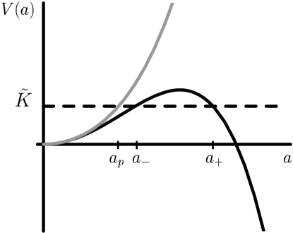
Figure 1: This figure shows the potencial $V(a)$ defined on Eq. (3). The darkest and lightest curves correspond to a positive and negative cosmological constant $\Lambda=3\lambda$ cases, respectively. The parameter $\tilde{K}$ is related to the amount of radiation presents in the FRW universe. On the one hand, for positive $\lambda$ and $\tilde{K}$ smaller than the maximum of $V(a)$, as in the case plotted, $a_{-}$ represents the maximum radius of the collapsing radiation-filled FRW universe, while $a_{+}$ represents the minimum scale factor of the asymptotically de Sitter universe. On the other hand, for negative $\lambda$ the scale factor $a_{p}$ represents the maximum radius of the collapsing universe.

The shape of the potential $V(a)$ depends on the sign of the cosmological constant $\lambda$. For a positive cosmological constant, it increases up to a maximum value $\frac{1}{4\lambda}$ at $a=\frac{1}{\sqrt{2\lambda}}$, and decreases after that for scale factors larger than $\frac{1}{\sqrt{2\lambda}}$ Fig. (1). For a negative cosmological constant the situation is rather different, as the potential is always increasing and never negative Fig. (1).

We can distinguish three kinds of behavior for $a$. The first one describes a collapsing universe. This is the case when the cosmological constant is negative and $\tilde{K}\neq 0$, for which

$$a(\bar{\eta})=a_{p}{\rm cn}\left[\sqrt{m}(\bar{\eta}-\bar{\eta}_{+}),\frac{m-1}{2m}\right],$$ (4)

where $\bar{\eta}\in[\bar{\eta}_{-},\bar{\eta}_{+}]$, $a_{p}^{2}=\frac{1-m}{2\lambda}$, $m=\sqrt{1-4\tilde{K}\lambda}$ and $\sqrt{m}(\bar{\eta}_{+}-\bar{\eta}_{-})={\rm K}(\frac{m-1}{2m})$. In these expressions, ${\rm cn}[x,\frac{m-1}{2m}]$ is a Jacobian Elliptic function and ${\rm K}(\frac{m-1}{2m})$ is the complete Jacobian elliptic integral or quarter-period function Abramowitz ; Gradshteyn . Note that $\bar{\eta}_{+}$ is an arbitrary constant that can be set equal to zero. The scale factor of this universe increase from $a=0$ at $\bar{\eta}=\bar{\eta}_{-}$ up to $a=a_{p}$ for $\bar{\eta}=0$, which is the maximum radius of this universe. The other case of a collapsing closed FRW universe corresponds to a positive cosmological constant and a value of the parameter $\tilde{K}$, related to the amount of radiation present in the universe, smaller than the maximum of the potential $V(a)$, i.e., $0<\tilde{K}<\frac{1}{4\lambda}$. Under these conditions, the scale factor in terms of the cosmological time, $d\bar{t}=a(\bar{\eta})d\bar{\eta}$, has the expression

$$a(\bar{t})^{2}=\frac{1}{2\lambda}\left\{1-m\cosh\left[2\sqrt{\lambda}(\bar{t}-\bar{t}_{-})\right]\right\},$$

the maximum value of the scale factor is $a_{-}^{2}=\frac{1-m}{2\lambda}$, the corresponding to $\bar{t}=\bar{t}_{-}$ which is the solution of the algebraic equation $V(a)=\tilde{K}$. For both solutions, the maximum radius of the universe increases with the amount of radiation, given by $\tilde{K}$.

The second kind of solutions describes an asymptotically de Sitter space-time when $\lambda>0$, whose scale factor is given by

$$a(\bar{t})^{2} = \frac{1}{2\lambda}\left\{\sqrt{4\tilde{K}\lambda}\sinh\left[2\sqrt{\lambda}(\bar{t}-\bar{t}_{+})\right]-\right.$$

$$- \left.\cosh\left[2\sqrt{\lambda}(\bar{t}-\bar{t}_{+})\right]+1\right\}$$

for $\tilde{K}>\frac{1}{4\lambda}$, and

$$a(\bar{t})^{2}=\frac{1}{2\lambda}\left\{1+m\cosh\left[2\sqrt{\lambda}(\bar{t}-\bar{t}_{+})\right]\right\},$$

for $\tilde{K}<\frac{1}{4\lambda}$, where $\bar{t}\in[\bar{t}_{+},+\infty)$. The difference between these two cases is that for sufficient radiation, i.e. $\tilde{K}$ is larger than the maximum of the potential $V(a)$, the scale factor grows from zero up to infinity, while in the opposite case; i.e. for $\tilde{K}$ smaller than the maximum of the potential $V(a)$, the scale factor grows from a minimum value different from zero, $a_{+}^{2}=\frac{1+m}{2\lambda}$, due to the presence of the barrier of potential $V(a)$, to become asymptotically de Sitter.

And finally, there is a third kind of solutions which exactly coincides with a de Sitter space-time

$$a(\bar{t})^{2}=\frac{1}{\lambda}\cosh^{2}\left[\sqrt{\lambda}(\bar{t}-\bar{t}_{+})\right],$$

in the absence of radiation and for a positive $\lambda$.

It can be checked that there are not classical solutions of the Einstein equations corresponding to a closed FRW in absence of radiation, $\tilde{K}=0$, with a negative cosmological constant. It is only for $\tilde{K}>0$ that it is possible to have a Lorentzian evolution for the scale factor $a$.

Up to now, we have described the different possible Lorentzian solutions for a closed homogeneous and isotropic universe filled with radiation and we have seen that the potential $V(a)$ forbids the classical evolution for some values of the scale factor. Therefore two classical FRW universes filled with radiation with $\tilde{K}<\frac{1}{4\lambda}$ are disconnected and the scale factor for a FRW universe with a negative cosmological constant has a maximum value when the content of the universe corresponds to radiation.

As it is well known, the fact that two classically allowed universes separated by a potential barrier are classically disconnected does not mean that they cannot be connected quantum mechanically. In the lowest approximation, this connection is established by an instanton whose explicit form can be obtained by performing an analytical continuation of Eq. (2), for a positive $\lambda$, so that the classically forbidden region is now the permitted one. The solution for the scale factor must satisfy

$$a(\eta_{-})=a_{-},\qquad a(\eta_{+})=a_{+},$$

in order to connect with the two classical FRW universes. From the analytically continued version of Eq. (2), we obtain the following solution for the scale factor:

$$a(\eta)^{2}=\frac{1+m}{2\lambda}\;{\rm dn}^{2}\left[\sqrt{\frac{1+m}{2}}(\eta-\eta_{+}),\frac{2m}{1+m}\right],$$ (5)

where $\eta\in[\eta_{-},\eta_{+}]$ with $\eta_{+}-\eta_{-}=-\sqrt{\frac{2}{1+m}}{\rm K}(\frac{2m}{1+m})$. In this expression ${\rm dn}[x,\frac{2m}{1+m}]$ is the Jacobian elliptic delta-amplitude function Abramowitz ; Gradshteyn . Note that $\eta_{+}$ is an arbitrary constant that can be set equal to zero. This instanton was also found in Ref. Halliwell , where the authors considered a closed FRW with a material content corresponding to a massless scalar field conformally coupled to gravity. In the absence of radiation, $m=1$, the turning points of the potential $V(a)$, i.e., the solution of $V(a)=\tilde{K}$, (see Eq. (3)) becomes $a_{-}=0$, $a_{+}=\sqrt{1/\lambda}$. The instanton (5) then acquires the simple form

$$a(\eta)^{2}=\frac{1}{\lambda}{\rm sech}^{2}(\eta-\eta_{+})$$

and $\eta_{+}-\eta_{-}=\infty$.

While for a positive cosmological constant the Euclidean solution for a closed FRW universe filled with radiation connects two classical solutions, for a negative $\lambda$ the solution behaves as an Euclidean asymptotically anti de Sitter wormhole. This can be easily deduced from the analytical continuation of Eq. (2) to imaginary conformal time. The scale factor of the wormhole looks like Barcelo1

$$a(\eta)^{2}=a_{p}^{2}{\rm nc}^{2}\left[\sqrt{m}(\eta-\eta_{-}),\frac{1+m}{2m}\right],$$ (6)

where $\eta\in[\eta_{-},\eta_{+}]$ and $\sqrt{m}(\eta_{+}-\eta_{-})={\rm K}(\frac{1+m}{2m})$. In this expression ${\rm nc}[x,\frac{1+m}{2m}]$ is a Jacobian Elliptic function Abramowitz ; Gradshteyn . The value $a_{p}$ describes the radius of the wormhole throat.

III The wave function of the universe

The quantum behavior of the FRW universe can be described by the solution to the Wheeler-DeWitt equation Wheeler . In the WBK approximation, the wave functions can be approximated, under certain conditions, by ingoing and outgoing modes defined through the classical action in the Lorentzian section, while in the Euclidean sector, the wave function can be approximated by linear combinations of increasing and decreasing modes in terms of the Euclidean action. Boundary conditions that determine these linear combinations are also necessary. In this section, we will obtain the general shape of the wave function of a closed FRW universe filled with radiation and whose content corresponds to a massive scalar field conformally coupled to gravity.

III.1 Canonical formulation

We will consider a minisuperspace described by two degrees of freedom, the scale factor $a$ and a homogeneous and isotropic scalar field conformally coupled to gravity $\tilde{A}$. Around this minisuperspace, we will study the linear perturbations due to an inhomogeneous and anisotropic massive scalar field $\Phi$ conformally coupled to gravity. We will obtain the Wheeler-DeWitt equation from a specific representation of the Hamiltonian of the system which can be constructed easily from the classical action of the system

$$S = S_{{\rm g}}+S_{\rm r}+S_{\rm m},$$

$$S_{{\rm g}} = {\frac{1}{16\pi{\rm G}}\int d^{4}x\sqrt{-g}\left(R-6\lambda\right)}-$$

$$- {\frac{1}{8\pi{\rm G}}\int d^{3}x\sqrt{h}K},$$

$$S_{{\rm r}} = {\int d^{4}x\sqrt{-g}\left[-\frac{1}{2}(\nabla\tilde{A})^{2}-\frac{1}{12}R\tilde{A}^{2}\right]}+$$

$$+ {\frac{1}{6}\int d^{3}x\sqrt{h}K\tilde{A}^{2}},$$

$$S_{{\rm m}} = {\int d^{4}x\sqrt{-g}\left[-\frac{1}{2}\nabla\Phi^{2}-\frac{1}{2}\left(\mu^{2}+\frac{1}{6}R\right)\Phi^{2}\right]}+$$ (7)

$$+ \frac{1}{6}\int d^{3}x\sqrt{h}K\Phi^{2},$$

where ${\rm G}$ is the gravitational constant, $\mu$ is the mass of the scalar field and $K$ is the trace of the extrinsic curvature. We have used the sign of conventions of Misner, Thorne and Wheeler Misner .

We introduce new variables which correspond to an expansion in hyperspherical harmonics of the massive scalar field around the background solution described in the previous section as follows

$$\Phi({\mathbf{x}},\bar{\eta}) = a(\bar{\eta})^{-1}\bigg{[}\varphi(\bar{\eta})+\sum_{nlm}f_{nlm}(\bar{\eta})Q^{nlm}({\mathbf{x}})\bigg{]}$$ (8)

$$\tilde{A}({\mathbf{x}},\bar{\eta}) = \frac{1}{\sqrt{2\pi}}a(\bar{\eta})^{-1}\bigg{[}\tilde{\chi}(\bar{\eta})+\sum_{nlm}\zeta_{nlm}(\bar{\eta})Q^{nlm}({\mathbf{x}})\bigg{]}$$

where $Q^{nlm}$ are the scalar hyperspherical harmonics, eigenfunctions of the 3-dimensional Laplacian $\nabla^{2}$ in the three-sphere, i.e., they satisfy the eigenvalue equation $\nabla^{2}Q^{nlm}=-n(n+2)Q^{nlm}$, with $n=0,1,2,\dots$. The mode $n=0$ corresponds to the homogeneous and isotropic perturbation, while higher values of $n$ correspond to inhomogeneous and anisotropic modes. We have considered the background solution of the massive scalar field $\Phi$, equal to zero, i.e. $\varphi=0$. From now on and for the sake of simplicity, we will drop the indices $lm$ and keep only the eigenvalue index $n$ in all the expressions.

The space-time metric must also be expanded around the homogeneous and isotropic background solution. If we write the Lorentzian metric in the $3+1$ form

$$ds^{2}=a^{2}(-N^{2}+N^{i}N_{i})d\eta^{2}+2aN_{i}d\eta dx^{i}+g_{ij}dx^{i}dx^{j},$$

this expansion can be written as

$$N = 1+\sum_{n}g_{n}Q^{n},$$

$$N_{i} = \sum_{n}(j_{n}P^{n}_{i}+k_{n}S^{n}_{i}),$$

$$g_{ij} = a^{2}(\Omega_{ij}+\epsilon_{ij}),$$

$$\epsilon_{ij} = \sum_{n}(a_{n}Q^{n}_{ij}+b_{n}P^{n}_{ij}+c_{n}S^{n}_{ij}+d_{n}G^{n}_{ij}),$$

$\Omega_{ij}$ being the metric in the unit three-sphere and ${Q^{n}}$, ${P^{n}}$, ${S^{n}}$ and ${G^{n}}$ are the standard hyperspherical harmonics on the three-sphere Lifshitz ; hawking .

The coefficients $x_{n}\equiv\{a_{n},b_{n},c_{n},g_{n},j_{n},k_{n}\}$ can in principle be eliminated by means of a diffeomorphism on the three-sphere and choosing suitable lapse and shift functions hawking ; wada . The only terms in these expansions that cannot be gauged away correspond to pure transverse traceless tensor perturbations that describe gravitational waves. These are represented by the coefficients $d_{n}$. The Lorentzian action up to second order in perturbations has the form

$$S=S^{(0)}[a,\chi]+S_{g+r}^{(2)}[a,\chi,\zeta_{n},x_{n},d_{n}]+S_{m}^{(2)}[a,f_{n}].$$

This can be seen from Eq. (7) taking into account that the massive background field vanishes; i.e. $\varphi=0$. Indeed in this case the perturbations of the massive scalar field decouple from perturbations of the metric and the radiation up to second order. Since we are interested in the behavior of closed FRW universes against the quantum fluctuations of the vacuum of the massive scalar field $\Phi$, we have chosen its homogeneous background mode to vanish. So the explicit expression of $S_{g+r}^{(2)}$ is not necessary to study the behavior of the FRW universe under perturbations of the massive scalar field. The zero order action $S^{(0)}$ and the second order action of the scalar field perturbations $S_{m}^{(2)}$ have the form

$$S^{(0)}[a,\chi] = \int_{\bar{\eta}_{-}}^{0}d\bar{\eta}\left[\frac{3\pi}{4\rm{G}}(a^{2}-a^{\prime 2}-\lambda a^{4})+\frac{\pi}{2}(\tilde{\chi}^{\prime 2}-\tilde{\chi}^{2})\right],$$

$$S^{(2)}_{\rm m}[a,f_{n}] = \sum_{n}\int_{\bar{\eta}}^{0}d\bar{\eta}\left(\frac{1}{2}f_{n}^{\prime 2}-\frac{1}{2}U_{n}(\bar{\eta})f_{n}^{2}\right),$$ (10)

where

$$U_{n}(\bar{\eta})=(n+1)^{2}+\mu^{2}a(\bar{\eta})^{2}.$$

Finally, the Hamiltonian of the system can be written as

$$H = H^{(0)}[a,\chi]+H^{(2)}_{\rm m}[a,f_{n}],$$

$$H^{(0)}[a,\chi] = -\frac{\rm{G}}{3\pi}\;P_{a}^{2}-\frac{3\pi}{4\rm{G}}a^{2}+\frac{3\pi}{4\rm{G}}\lambda a^{4}\;+\;\frac{1}{2}(P_{\tilde{\chi}}^{2}+\tilde{\chi}^{2}),$$

$$H^{(2)}_{\rm m}[a,f_{n}] = \sum_{n}\frac{1}{2}P_{f_{n}}^{2}+\frac{1}{2}U_{n}(\bar{\eta})f_{n}^{2}.$$ (11)

This Hamiltonian describes the classical constraint of our system $H=0$ and is related with the invariance of the Lorentzian action under time reparametrizations. This constraint will be our starting point for studying the quantum behavior of closed FRW universes filled with radiation.

The constraint $H=0$ in the context of quantum gravity becomes a constraint on the wave function of the universe leading to the Wheeler-DeWitt equation, which can be written as

$$\displaystyle\left\{-\frac{\textrm{G}}{3\pi}\partial^{2}_{a}+\frac{3\pi}{4\textrm{G}}(a^{2}-\lambda a^{4})+\frac{1}{2}(\partial^{2}_{\tilde{\chi}}-\tilde{\chi}^{2})+\right.$$ (12)

$$\left.\displaystyle{\frac{1}{2}\sum_{n=1}^{+\infty}\left\{\partial^{2}_{f_{n}}-U_{n}(a)f_{n}^{2}\right\}}\right\}\widetilde{\Psi}(a,f_{n},\tilde{\chi})=0$$ ,

where

$$U_{n}(a)=(n+1)^{2}+\mu^{2}a^{2}.$$

The functional dependence of the wave function on the radiation field can be obtained by separation of variables. The part of the wave function $\Psi(a,f_{n})$ which depends on the other degrees of freedom present in our model, $a$ and $f_{n}$, must satisfy

$$\left[-\frac{\textrm{G}}{3\pi}\partial^{2}_{a}+\frac{3\pi}{4\textrm{G}}V_{0}(a)+\sum_{n=1}^{+\infty}(\frac{1}{2}\partial^{2}_{f_{n}}-V_{n}(a)f_{n}^{2})\right]\Psi(a,f_{n})=0,$$ (13)

where the potentials $V_{n}(a)$ and $V_{0}(a)$ are defined as follows:

$$V_{n}(a) = \frac{1}{2}[(n+1)^{2}+\mu^{2}a^{2}],\;n=1,2,\ldots,$$

$$V_{0}(a) = a^{2}-\lambda a^{4}-\tilde{K}.$$ (14)

Here $\tilde{K}$ is a separation constant, related to the energy of the mode $\tilde{\chi}$ and quantifies the amount of radiation present in the universe as we have seen in Sec. II.

III.2 Semiclassical approximation

We will treat the quantum behavior of radiation-filled FRW in the semiclassical approximation wada ; Vilenkin2 , where the physical lengths involved in our problem are larger than Planck length $l_{p}$. In this approximation, the solutions to equation (13) will be written as linear combinations of

$$\Psi_{1}(a,f_{n})=\exp\left[-\frac{1}{\textrm{G}}S_{0}(a)-\frac{1}{2}\sum_{n=1}^{+\infty}S_{n}(a)f_{n}^{2}\right],$$

$$\Psi_{2}(a,f_{n})=\exp\left[-\frac{1}{\textrm{G}}R_{0}(a)-\frac{1}{2}\sum_{n=1}^{+\infty}R_{n}(a)f_{n}^{2}\right],$$ (15)

where $\Psi_{1}$ and $\Psi_{2}$ will be decreasing and increasing functions in the classically forbidden regime or ingoing and outgoing waves in the classically allowed regime Vilenkin2 . We will deal firstly with the regions of validity of the semiclassical approximation in term of the amount of radiation present in the universe and in later stage of our study, we will specify clearly the kind of functions on each regime, they will depend on the inclusion of the Lorentzian or the Euclidean time. $S_{0}$ and $R_{0}$ are related to the unperturbed part of the wave function of the universe while $S_{n}$ and $R_{n}$ are related to the vacuum fluctuations of the massive scalar field and corresponds to the perturbative part of the wave function of the universe. Using the WBK approximation, we obtain

$$\left(\frac{dS_{0}}{da}\right)^{2}=\frac{9\pi^{2}}{4}V_{0}(a),$$ (16)

$$\frac{dS_{0}}{da}\frac{dS_{n}}{da}-\frac{3\pi}{2}S_{n}^{2}=-3\pi V_{n}.$$ (17)

where we have performed an asymptotic expansion on G and likewise for $R_{0}$ and $R_{n}$. Similarly to the usual WBK this approximation is valid as long as

$$\textrm{G}|\frac{dV_{0}(a)}{da}|\ll|V_{0}(a)|^{\frac{3}{2}}.$$ (18)

From now on, we will consider that the amount of radiation present on the closed FRW universes in the case of positive cosmological constant $\lambda$, is such that this kind of models has two classically disconnected solutions, i.e. $0<\tilde{K}<1/4\lambda$, allowing for quantum tunelling between the two universes. As can be seen from the validity of the WBK approximation Eq. (18), this condition breaks down near the points $a_{-}$ and $a_{+}$ in the case of $\lambda>0$. These points corresponds respectively to the maximum radius of the collapsing universe and the minimum radius of the asymptotically de Sitter universe. Similarly the WBK method is not valid near the point $a_{p}$ which corresponds to the maximum radius of the collapsing universe in the case of a negative $\lambda$. Therefore we have to analyze the behavior of the wave function near these turning points using other methods as explained below.

III.3 Turning points

Starting from the expansion of the potentials $V_{0}(a)$ and $V_{n}(a)$ around each turning point, $a_{-}$, $a_{+}$ and $a_{p}$, the Wheeler-DeWitt equation (13) acquires the form

$$\left\{-\frac{\textrm{G}}{3\pi}\partial^{2}_{a}+\frac{3\pi}{4\textrm{G}}\frac{dV_{0}(a)}{da}|_{a=a_{i}}(a-a_{i})\right.$$

$$\left.+\sum_{n=1}^{+\infty}\left[\frac{1}{2}\partial^{2}_{f_{n}}-V_{n}(a_{i})f_{n}^{2}\right]\right\}\Psi(a,f_{n})=0,$$ (19)

where $a_{i}=a_{\pm},a_{p}$. This linear approximation hold if and only if:

$$|(a-a_{i})\frac{d^{2}V_{0}(a)}{d^{2}a}|_{a=a_{i}}|\ll 2|\frac{dV_{0}(a)}{da}|_{a=a_{i}}.$$ (20)

The wave functions of the closed FRW universes can be expressed as linear combinations of $\Psi_{1}(a,f_{n})$ and $\Psi_{2}(a,f_{n})$ defined in Eq. (15), where $S_{0}$, $R_{0}$, $S_{n}$ and $R_{n}$ satisfy the differential equations (16,17), if the value of the scale factor, $a$, is such that the condition (18) holds. While in the linear regime the behavior of the wave functions of these universes will be solution of Eq. (19). As we will see there are values of the radius of the universe where both conditions Eqs. (18,20) hold and it is possible to connect the wave function on the WBK regimes through the linear regime.

Let us begin analyzing the case of a positive cosmological constant, in which the conditions for the linear approximation are

$$|a-a_{+}|\ll\frac{2m}{2+3m}a_{+},\;|a-a_{-}|\ll|\frac{2m}{-2+3m}|\;a_{-}$$

respectively around $a_{+}$ and $a_{-}$, while near these turning points the WBK conditions (18) read:

$$\textrm{G}^{2/3}(2a_{+}m)^{-1/3}\ll|a-a_{+}|,$$

$$\textrm{G}^{2/3}(2a_{-}m)^{-1/3}\ll|a-a_{-}|,$$ (22)

where the first one corresponds to $a_{+}$ and the second one to $a_{-}$. So it is a sufficient condition that

$$(\textrm{G}\lambda)^{2}\ll|\frac{4m^{4}(1+m)^{2}}{(2+3m)^{3}}|,$$

$$(\textrm{G}\lambda)^{2}\ll|\frac{4m^{4}(1-m)^{2}}{(-2+3m)^{3}}|,$$ (23)

to conclude the existence of values of $a$ such that there exists an overlapping between the WBK and the linear approximations. This overlapping depends only on the amount of radiation present in the FRW universes when it can be described semiclassically $\lambda\ll\textrm{G}^{-1}$.

In the case of a negative cosmological constant $\lambda<0$, we have to deal with a unique turning point $a_{p}$. Using similar methods to the case $\lambda>0$, we obtain that a sufficient condition for the existence of value of $a$ such that the linear and WBK approximation hold is:

$$(\textrm{G}\lambda)^{2}\ll\frac{4m^{4}(m-1)^{2}}{(3m-2)^{3}},$$ (24)

which is the case when the maximum value of the radius of the collapsing closed FRW universe, $a_{p}$, is large enough (equivalently the parameter $m$ is large).

IV Matching conditions

Using the fact that there are values of the scale factor, $a$, in which the linear and WBK approximations hold, we will connect the wave function on the different WBK regimes through the linear ones around the turning points, $a_{-}$, $a_{+}$ and $a_{p}$.

IV.1 Positive cosmological constant

For the case of a positive cosmological constant there are three WBK regimes, one corresponding to values of the scale factor such that $a<a_{-}$ and the wave function, $\Psi_{{\text{i}}}$, can be written as

$$\Psi_{{\text{i}}}(a,f_{n}) = C\exp\left[-\frac{1}{\textrm{G}}S^{{\text{i}}}_{0}(a)-\frac{1}{2}\sum_{n=1}^{+\infty}S^{{\text{i}}}_{n}(a)f_{n}^{2}\right]+$$

$$+ D\exp\left[-\frac{1}{\textrm{G}}R^{{\text{i}}}_{0}(a)-\frac{1}{2}\sum_{n=1}^{+\infty}R^{{\text{i}}}_{n}(a)f_{n}^{2}\right];$$

a second one, which is classically forbidden, $a_{-}<a<a_{+}$, and for which the wave function, $\Psi_{{\text{ii}}}$, can be expressed as follows

$$\Psi_{{\text{ii}}}(a,f_{n}) = A\exp\left[-\frac{1}{\textrm{G}}S^{{\text{ii}}}_{0}(a)-\frac{1}{2}\sum_{n=1}^{+\infty}S^{{\text{ii}}}_{n}(a)f_{n}^{2}\right]+$$

$$+ B\exp\left[-\frac{1}{\textrm{G}}R^{{\text{ii}}}_{0}(a)-\frac{1}{2}\sum_{n=1}^{+\infty}R^{{\text{ii}}}_{n}(a)f_{n}^{2}\right];$$

and finally, a third one in which the scale factor, $a$, is larger than $a_{+}$. In this regime the wave function is

$$\Psi_{{\text{iii}}}(a,f_{n}) = E\exp\left[-\frac{1}{\textrm{G}}S^{{\text{iii}}}_{0}(a)-\frac{1}{2}\sum_{n=1}^{+\infty}S^{{\text{iii}}}_{n}(a)f_{n}^{2}\right]+$$

$$+ F\exp\left[-\frac{1}{\textrm{G}}R^{{\text{iii}}}_{0}(a)-\frac{1}{2}\sum_{n=1}^{+\infty}R^{{\text{iii}}}_{n}(a)f_{n}^{2}\right].$$

In all these expressions, the functions with the subscript $0$ represent the background part of the wave function and satisfy the differential equation (16), while the functions with suffix $n$, $n\geq 1$, correspond to the perturbations of the wave function of the universe and they are solutions of the differential equation stated in expression (17). Outside the potential barrier $V(a)$, the functions $S_{0}^{{\text{i}}}$ and $S_{0}^{{\text{iii}}}$ are related to the outgoing modes and the functions $R_{0}^{{\text{i}}}$ and $R_{0}^{{\text{iii}}}$ correspond to the ingoing modes. On the other hand, under the potential barrier $S_{0}^{{\text{ii}}}$ and $R_{0}^{{\text{ii}}}$ represent growing and decreasing background terms, respectively, of the wave function $\Psi_{{\text{ii}}}$.

To connect the wave function of the FRW universe Eqs. (LABEL:funcion1,LABEL:funcion2,LABEL:funcion3) through the linear regimes around $a_{-}$ and $a_{+}$ we will consider that we have a unique mode $f_{n}$ of the massive scalar field $\Phi$. The general case can be easily deduced from this one. Near the turning points, the wave function of the closed FRW universe filled with radiation and a positive cosmological constant in addition to the vacuum fluctuation of a massive conformally coupled scalar field, can be expressed as

$$\Psi_{i}(a,f_{n}) = \sum_{m_{i}=0}^{+\infty}\left[\gamma_{m_{i}}Ai(z_{i})+\delta_{m_{i}}Bi(z_{i})\right]\times$$ (28)

$$\times \exp(-y_{n_{i}}^{2}/2){\rm H}_{m_{i}}(y_{n_{i}}),$$

where

$$z_{i} = (-1)^{i+1}\left(\frac{3\pi}{2\textrm{G}}\right)^{2/3}\left[(-1)^{i+1}\partial_{a}{V}_{0}(a_{\mp})\right]^{1/3}(a-a_{\mp})+$$

$$+ 2\left(\frac{2\textrm{G}}{3\pi}\right)^{1/3}\left[(-1)^{i+1}\partial_{a}{V}_{0}(a_{\mp})\right]^{-2/3}\beta_{n_{i}},$$

$$\beta_{n_{i}} = -(2m_{i}+1)\sqrt{V_{n}(a_{\pm})/2};\;m_{i}\in\mathbb{N},$$

$$y_{n_{i}} = \left(2V_{n}(a_{\pm})\right)^{1/4}f_{n}.$$ (29)

in this expressions the index $i$ may takes the values 1 or 2 which correspond to the wave function on the linear regimes around $a_{-}$ and $a_{+}$ respectively, the potential $V_{0}(a)$ was defined in Eq. (14), $\gamma_{m_{i}}$ and $\delta_{m_{i}}$ are constants, the functions $Ai(x)$ and $Bi(x)$ are the Airy functions and ${\rm H}_{m_{i}}(x)$ are the Hermite’s polynomials Abramowitz .

Let us now begin connecting the WBK wave function under the barrier, $\Psi_{{\text{ii}}}(a,f_{n})$, around $a_{-}$ with the linear regime using the fact that there are values of the scale factor $a$, such that both approximations, the WBK and the linear one, hold as was explained in Sec. III.3. For these values of the scale factor, the wave function $\Psi_{{\text{ii}}}(a,f_{n})$, using Eqs. (16,LABEL:funcion2), can be expressed near $a_{-}$ as

$$\Psi_{{\text{ii}}}(a,f_{n}) = A\exp\left[\frac{\pi}{\textrm{G}}\sqrt{\partial_{a}{V}_{0}(a_{-})}\;(a-a_{-})^{3/2}\right]\times$$ (30)

$$\times \exp\left(-\frac{1}{2}S^{{\text{ii}}}_{n}(a_{)}f_{n}^{2}\right)+$$

$$+ B\exp\left[-\frac{\pi}{\textrm{G}}\sqrt{\partial_{a}{V}_{0}(a_{-})}\;(a-a_{-})^{3/2}\right]\times$$

$$\times \exp\left(-\frac{1}{2}R^{{\text{ii}}}_{n}(a_{)}f_{n}^{2}\right).$$

Let us do some remarks about the behavior of the variables $z_{i}$. These variables are related to the different indices $m_{i}$ of the Hermite’s polynomials, through the constants $\beta_{n_{i}}$ Eq. (29). Consequently, the functions $Ai(z_{i})$ and $Bi(z_{i})$ can not be factor out from the sums over the different indices $m_{i}$ which define the wave functions $\Psi_{i}$ near the turning points. However, since we are working on the semiclassical framework the second term, which is proportional to $\beta_{n_{i}}$, on the definition of $z_{i}$ is much smaller than the first one, as the first one is proportional to $\textrm{G}^{-2/3}$ while the second one is proportional to $\textrm{G}^{1/3}$. So the variables $z_{i}$ in this regime effectively do not depend on the indices $m_{i}$ and the Airy functions can be factor out from the sum given in Eq. (28). Considering our last statement, we will connect the wave function on the linear regime with that of the WBK regime for values of $z_{i}$ such that the Airy functions can be approximated by their asymptotic behaviors ($z_{i}\rightarrow\pm\infty$).

Near the turning point $a_{-}$, the variable $z_{1}$ is positive under the barrier and reaches values large enough to use the asymptotic behavior of the Airy functions. Once the $Ai(z_{1})$ and $Bi(z_{1})$ have been substituted by their asymptotic behavior in expression (28) for $i=1$, comparing the resulting expression for the wave function of the universe $\Psi_{1}(a,f_{n})$ near the turning points $a_{-}$ for $a>a_{-}$ with the wave function $\Psi_{{\text{ii}}}(a,f_{n})$ in Eq. (30), and imposing the continuity of the FRW wave function, we see that the growing term in $\Psi_{{\text{ii}}}$, related to $S^{{\text{ii}}}_{0}$, overlaps with the $Bi(z_{1})$ terms on the expression of $\Psi_{1}$, while the decreasing term in $\Psi_{{\text{ii}}}$, related to $R^{{\text{ii}}}_{0}$, overlaps with the $Ai(z_{1})$ terms on the expression of $\Psi_{1}$. Also we obtain the following equations

$$\sum_{m_{1}=0}^{+\infty}\gamma_{m_{1}}\exp\left(-\frac{y^{2}_{n_{1}}}{2}\right)H_{m_{1}}(y_{n_{1}})=$$

$$B\exp\left[-\frac{1}{2}R^{{\text{ii}}}_{n}(a_{-})f^{2}_{n}\right],$$

$$\sum_{m_{1}=0}^{+\infty}\delta_{m_{1}}\exp\left(-\frac{y^{2}_{n_{1}}}{2}\right)H_{m_{1}}(y_{n_{1}})=$$

$$A\exp\left[-\frac{1}{2}S^{{\text{ii}}}_{n}(a_{-})f^{2}_{n}\right].$$ (31)

(32)

Using the orthogonality relations of the Hermite polynomials Abramowitz and the following formula Gradshteyn :

$$\int_{-\infty}^{+\infty}\exp(-x^{2})H_{2m}(xy)dx=\sqrt{\pi}\frac{(2m)!}{m!}(y^{2}-1)^{m},$$ (33)

we have

$$\gamma_{m_{1}}=\left\{\begin{array}[]{ll}B(1-k_{-})^{l_{1}}/(2^{2l_{1}}{l_{1}}!k_{-}^{l_{1}+1/2}),\;m_{1}=2l_{1},\;l_{1}\in\mathbb{N}\\ 0,\qquad\qquad\qquad\qquad\qquad\;m_{1}=2l_{1}+1,\;l_{1}\in\mathbb{N},\end{array}\right.$$

$$\delta_{m_{1}}=\left\{\begin{array}[]{ll}A(1-\tilde{k}_{-})^{l_{1}}/(2^{2l_{1}}{l_{1}}!{\tilde{k}_{-}}^{l_{1}+1/2}),\;m_{1}=2l_{1},\;l_{1}\in\mathbb{N}\\ 0,\qquad\qquad\qquad\qquad\qquad\;m_{1}=2l_{1}+1,\;l_{1}\in\mathbb{N},\end{array}\right.$$

where

$$2k_{-}=\frac{R^{{\text{ii}}}_{n}(a_{-})}{\sqrt{2V_{n}(a_{-})}}+1,\;2\tilde{k}_{-}=\frac{S^{{\text{ii}}}_{n}(a_{-})}{\sqrt{2V_{n}(a_{-})}}+1.$$

The last expressions determine the linear behavior of the wave function near the point $a_{-}$ in terms of the WBK wave function under the barrier $V(a)$ (see Eq. (3)) which can be explicitly seen through the dependence of the coefficients $\delta_{m_{1}}$ and $\gamma_{m_{1}}$ in $A$ and $B$ respectively.

Now, using on the one hand the explicit expression of $\Psi_{1}(a,f_{n})$ around $a_{-}$ for values of the variable $z_{1}$ such that $z_{1}\rightarrow-\infty$ and on the another hand the behavior of the wave function $\Psi_{{\text{i}}}$ of the FRW universe outside the potential, $V(a)$ (see Eq. (3)), $\Psi_{{\text{i}}}(a,f_{n})$ near the turning point $a_{-}$, we can obtain similar relations to the ones expressed in Eq. (32) for the coefficients $\gamma_{m_{1}}$, $\delta_{m_{1}}$, $C$ and $D$:

$$\sum_{m_{1}=0}^{+\infty}\left(\gamma_{m_{1}}/(2i)-\delta_{m_{1}}/2\right)\exp(-i\frac{\pi}{4})\exp\left(-\frac{y^{2}_{n_{1}}}{2}\right)\times$$

$$\times H_{m_{1}}(y_{n_{1}})=C\exp\left[-\frac{1}{2}S^{{\text{i}}}_{n}(a_{-})f^{2}_{n}\right],$$

$$\sum_{m_{1}=0}^{+\infty}\left(\delta_{m_{1}}/2+\gamma_{m_{1}}/(2i)\right)\exp(i\frac{\pi}{4})\exp\left(-\frac{y^{2}_{n_{1}}}{2}\right)\times$$

$$\times H_{m_{1}}(y_{n_{1}})=D\exp\left[-\frac{1}{2}R^{{\text{i}}}_{n}(a_{-})f^{2}_{n}\right],$$

(34)

where we have used the continuity of the wave function of the FRW universe. Finally using expressions (32,34), we deduce

$$C = \left[A/2-B/(2i)\right]\exp\left(-i\frac{\pi}{4}\right),$$

$$D = \left[A/2+B/(2i)\right]\exp\left(i\frac{\pi}{4}\right),$$

$$S^{{\text{i}}}_{n}(a_{-}) = S^{{\text{ii}}}_{n}(a_{-})=R^{{\text{i}}}_{n}(a_{-})=R^{{\text{ii}}}_{n}(a_{-}),$$ (35)

which determine the wave function of a FRW universe filled with radiation outside the potential barrier $V(a)$, in terms of the wave function of a FRW universe inside the potential barrier $V(a)$ and viceversa.

Once we have obtained the matching conditions for the wave function in the case of a positive cosmological constant for the turning point $a_{-}$, let us deal with the matching conditions for the turning point $a_{+}$. For this purpose, we approximate the wave function, under the potential barrier $V(a)$, $\Psi_{{\text{ii}}}(a,f_{n})$ defined in Eq. (LABEL:funcion2) near the point $a_{+}$ by

$$\Psi_{{\text{ii}}}(a,f_{n})=$$

$$=A\exp\bigg{[}\frac{3\pi}{2\textrm{G}}\int_{a_{-}}^{a_{+}}\sqrt{V_{0}(a)}da-\frac{\pi}{\textrm{G}}\sqrt{-\partial_{a}{V}_{0}(a_{+})}\times\bigg{.}$$

$$\times\bigg{.}(a_{+}\;-a)^{3/2}\bigg{]}\exp\left(-\frac{1}{2}S^{{\text{ii}}}_{n}(a_{+})f_{n}^{2}\right)+$$

$$+B\exp\bigg{[}-\frac{3\pi}{2\textrm{G}}\int_{a_{-}}^{a_{+}}\sqrt{V_{0}(a)}da+\frac{\pi}{\textrm{G}}\sqrt{-\partial_{a}{V}_{0}(a_{+})}\times\bigg{.}$$

$$\times\bigg{.}(a_{+}\;-a)^{3/2}\bigg{]}\exp\left(-\frac{1}{2}R^{{\text{ii}}}_{n}(a_{+})f_{n}^{2}\right).$$ (36)

In the next step, we will match the wave function $\Psi_{{\text{ii}}}(a,f_{n})$, using the last equation, with the wave function on the linear regime around $a_{+}$, $\Psi_{2}(a,f_{n})$ expressed in Eq. (28) for $i=2$. Similarly to our procedure for the matching conditions in $a_{-}$, we use the asymptotic behavior of the Airy’s functions in the expression of $\Psi_{2}(a,f_{n})$ for values of the scale factor, $a$, such that the condition $z_{2}\rightarrow+\infty$, the WBK approximation and the linear one hold and we obtain the following relations between the coefficients $\gamma_{m_{2}}$, $\delta_{m_{2}}$ and the constants $A$ and $B$

$$\sum_{m_{2}=0}^{+\infty}\gamma_{m_{2}}\exp\left(-\frac{y^{2}_{n_{2}}}{2}\right)H_{m_{2}}(y_{n_{2}})=$$ (37)

$$A\exp\left[\frac{3\pi}{2\textrm{G}}\int_{a_{-}}^{a_{+}}\sqrt{V_{0}(a)}da\right]\exp\left[-\frac{1}{2}S^{{\text{ii}}}_{n}(a_{+})f^{2}_{n}\right],$$

$$\sum_{m_{1}=0}^{+\infty}\delta_{m_{2}}\exp\left(-\frac{y^{2}_{n_{2}}}{2}\right)H_{m_{2}}(y_{n_{2}})=$$

$$B\exp\left[-\frac{3\pi}{2\textrm{G}}\int_{a_{-}}^{a_{+}}\sqrt{V_{0}(a)}da\right]\exp\left[-\frac{1}{2}R^{{\text{ii}}}_{n}(a_{+})f^{2}_{n}\right].$$

Using as before the orthogonality relations of the Hermite polynomials, we have

$$\gamma_{m_{2}}=\left\{\begin{array}[]{ll}A\Delta(1-k_{+})^{l_{2}}/(2^{2l_{2}}{l_{2}}!{k_{+}}^{l_{2}+1/2}),\;m_{2}=2l_{2},\\ 0,\qquad\qquad\qquad\qquad\qquad\qquad m_{2}=2l_{2}+1,\end{array}\right.$$

$$\delta_{m_{2}}=\left\{\begin{array}[]{ll}B\Delta^{-1}(1-\tilde{k}_{+})^{l_{2}}/(2^{2l_{2}}{l_{2}}!{\tilde{k}_{+}}^{l_{2}+1/2}),\;m_{2}=2l_{2},\\ 0,\qquad\qquad\qquad\qquad\qquad\qquad m_{2}=2l_{2}+1,\end{array}\right.$$

where

$$2k_{+}=\frac{S^{{\text{ii}}}_{n}(a_{+})}{\sqrt{2V_{n}(a_{+})}}+1,\;2\tilde{k}_{+}=\frac{R^{{\text{ii}}}_{n}(a_{+})}{\sqrt{2V_{n}(a_{+})}}+1,$$

$$\Delta=\exp\left[\frac{3\pi}{2\textrm{G}}\int_{a_{-}}^{a_{+}}\sqrt{V_{0}(a)}da\right],\;l_{2}\in\mathbb{N}.$$ (38)

These expressions define the behavior of the wave function $\Psi_{2}(a,f_{n})$ in the linear regime around the turning point $a_{+}$ in term of the WBK wave function $\Psi_{{\text{ii}}}(a,f_{n})$ under the potential barrier $V(a)$.

Using the asymptotic behavior of the wave function $\Psi_{2}(a,f_{n})$, this time for $z_{2}\rightarrow+\infty$, we can match the wave function of the linear regime around $a_{+}$ with the wave function $\Psi_{{\text{iii}}}(a,f_{n})$ outside the barrier of potential $V(a)$. The continuity of the wave function implies

$$\sum_{m_{2}=0}^{+\infty}\left(-\gamma_{m_{2}}/(2i)+\delta_{m_{2}}/2\right)\exp(-i\frac{\pi}{4})\exp\left(-\frac{y^{2}_{n_{2}}}{2}\right)\times$$

$$\times H_{m_{2}}(y_{n_{2}})=E\exp\left[-\frac{1}{2}S^{{\text{iii}}}_{n}(a_{+})f^{2}_{n}\right]$$

$$\sum_{m_{2}=0}^{+\infty}\left(\delta_{m_{2}}/2+\gamma_{m_{2}}/(2i)\right)\exp(i\frac{\pi}{4})\exp\left(-\frac{y^{2}_{n_{2}}}{2}\right)\times$$

$$\times H_{m_{2}}(y_{n_{2}})=F\exp\left[-\frac{1}{2}R^{{\text{iii}}}_{n}(a_{+})f^{2}_{n}\right],$$

and therefore

$$E = \left[-\frac{A}{2i}\exp\left(\frac{3\pi}{2\textrm{G}}\int_{a_{-}}^{a_{+}}\sqrt{V_{0}(a)}\right)\right.+$$

$$+ \left.\frac{B}{2}\exp\left(-\frac{3\pi}{2\textrm{G}}\int_{a_{-}}^{a_{+}}\sqrt{V_{0}(a)}\right)\right]\exp(-i\frac{\pi}{4}),$$

$$F = \left[\frac{A}{2i}\exp\left(\frac{3\pi}{2\textrm{G}}\int_{a_{-}}^{a_{+}}\sqrt{V_{0}(a)}\right)+\right.$$ (40)

$$+ \left.\frac{B}{2}\exp\left(-\frac{3\pi}{2\textrm{G}}\int_{a_{-}}^{a_{+}}\sqrt{V_{0}(a)}\right)\right]\exp(i\frac{\pi}{4}),$$

$$S_{n}^{{\text{ii}}}(a_{+})=S_{n}^{{\text{iii}}}(a_{+})=R_{n}^{{\text{ii}}}(a_{+})=R_{n}^{{\text{iii}}}(a_{+}).$$

These equalities, together with Eq. (35) are the matching conditions for the wave function of a FRW universe filled with radiation, a positive cosmological constant and the vacuum fluctuations of a massive conformally coupled scalar field. Apart from these matching conditions, there are other conditions which ensure the good behavior of the wave function. These are the regularity conditions Vilenkin2

$$\mathit{Re}\left[S_{n}^{{\text{i}}}(a)\right],\;\mathit{Re}\left[R_{n}^{{\text{i}}}(a)\right]>0, \;\textrm{for}\;a<a_{-},$$

$$\mathit{Re}\left[S_{n}^{{\text{ii}}}(a)\right],\;\mathit{Re}\left[R_{n}^{{\text{ii}}}(a)\right]>0, \;\textrm{for}\;a_{-}<a<a_{+},$$

$$\mathit{Re}\left[S_{n}^{{\text{iii}}}(a)\right],\;\mathit{Re}\left[R_{n}^{{\text{iii}}}(a)\right]>0, \;\textrm{for}\;a_{+}<a.$$ (41)

IV.2 Tunneling boundary conditions of the universe

As an example that illustrates the applications of these boundary condition, let us discuss the tunneling boundary conditions of the universe Vilenkin3 . For these boundary conditions, outside and far from the potential barrier $V(a)$, i.e. in the classically allowed region and for values of the scale factor much larger than the turning point $a_{+}$, the wave function of the universe should contain only outgoing modes. That is, the coefficient $F$ (see Eq. (LABEL:funcion3)) must be equal to zero, so that no ingoing modes appear on the asymptotically de Sitter region. Once the tunneling boundary conditions have been applied, we can deduce the linear combination of the growing and decaying terms that define the FRW wave function under the barrier, i.e. the relationship between the constants $A$ and $B$ (see Eq. (40))

$$|A/B|=\exp\left(-\frac{3\pi}{\textrm{G}}\int_{a_{-}}^{a_{+}}\sqrt{V_{0}(a)}\right),$$ (42)

in agreement with the results obtained in Ref. Barcelo2 for an analogous system.

So, both growing and decaying background terms are present in the expression of $\Psi_{{\text{ii}}}(a,f_{n})$ under the barrier $V(a)$. Nevertheless, we see that the growing term associated to $S_{0}^{{\text{ii}}}(a)$ is multiplied by the constant $A$ which is exponentially smaller than the constant $B$, which multiply the decreasing term on $\Psi_{{\text{ii}}}(a,f_{n})$. We see that, even if it allows the appearance of a growing term on the classically forbidden region, under the barrier, it is exponentially reduced. On the other hand the wave function $\Psi_{{\text{i}}}(a,f_{n})$ defined on the classically allowed collapsing region $a<a_{-}$, will be a combination a of ingoing and outgoing modes.

IV.3 Negative cosmological constant

In the case of a negative cosmological constant, $\lambda<0$, there is a unique turning point $a_{p}$. This value of the scale factor separates a classically allowed region, $a<a_{p}$, from a classically forbidden one, $a_{p}<a$. The matching conditions for the wave function around $a_{p}$ can be deduced carrying out a similar analysis to the one presented previously for $\lambda>0$. We summarize our results in what follows.

In the classically allowed region ($a<a_{p}$), we will denote the wave function by

$$\Psi_{{\text{a}}}(a,f_{n}) = A_{{\text{a}}}\exp\left[-\frac{1}{\textrm{G}}S^{{\text{a}}}_{0}(a)-\frac{1}{2}\sum_{n=1}^{+\infty}S^{{\text{a}}}_{n}(a)f_{n}^{2}\right]+$$

$$+ B_{{\text{a}}}\exp\left[-\frac{1}{\textrm{G}}R^{{\text{a}}}_{0}(a)-\frac{1}{2}\sum_{n=1}^{+\infty}R^{{\text{a}}}_{n}(a)f_{n}^{2}\right],$$

while in the forbidden region ($a_{p}<a$), the wave function will be

$$\Psi_{{\text{f}}}(a,f_{n})=\exp\left[-\frac{1}{\textrm{G}}S^{{\text{f}}}_{0}(a)-\frac{1}{2}\sum_{n=1}^{+\infty}S^{{\text{f}}}_{n}(a)f_{n}^{2}\right].$$ (44)

Where we have considered only the decreasing wave function for the asymptotic region $a_{p}<a$ under the barrier.

In the linear regime, around the scale factor $a=a_{p}$, the wave function satisfies Eq. (19) and can be expressed as

$$\Psi_{p}(a,f_{n}) = \sum_{m_{p}=0}^{+\infty}\left[\gamma_{m_{p}}Ai(z_{p})+\delta_{m_{p}}Bi(z_{p})\right]\times$$ (45)

$$\times \exp(-y_{n_{p}}^{2}/2){\rm H}_{m_{p}}(y_{n_{p}}),$$

where

$$z_{p} = \left(\frac{3\pi}{2\textrm{G}}\right)^{2/3}\left[\partial_{a}V_{0}(a_{p})\right]^{1/3}(a-a_{p})+$$

$$+ 2\left(\frac{2\textrm{G}}{3\pi}\right)^{1/3}\left[\partial_{a}V(a_{p})\right]^{-2/3}\beta_{n_{p}},$$

$$\beta_{n_{p}} = -(2m_{p}+1)\sqrt{V_{n}(a_{p})/2};m_{p}\in\mathbb{N},$$

$$y_{n_{p}} = \left(2V_{n}(a_{p})\right)^{1/4}f_{n},\;$$ (46)

We match the wave function in the linear regime (see Eq. (45)) with the wave function under the barrier $\Psi_{{\text{f}}}(a,f_{n})$ (see Eq. (44)), taking into account that the background part of $\Psi_{{\text{f}}}(a,f_{n})$ is a decreasing function of the scale factor $a$, whose exponent can be approximated near $a_{p}$ by

$$S^{{\text{f}}}_{0}(a)=\pi\sqrt{\partial_{a}{V}_{0}(a_{p})}(a-a_{p})^{\frac{3}{2}},$$ (47)

The background part of the FRW wave function outside the barrier $\Psi_{{\text{a}}}$ in the neighborhood of $a_{p}$ corresponds to ingoing and outgoing modes. Therefore $S_{0}^{{\text{a}}}$ and $R_{0}^{{\text{a}}}$ will have the form

$$S_{0}^{{\text{a}}}(a)=-R_{0}^{{\text{a}}}(a)=i\pi\sqrt{\partial_{a}{V_{0}}(a_{p})}(a_{p}-a)^{\frac{3}{2}}.$$ (48)

Taking into account that there exists values of the scale factor close to $a_{p}$ for which the linear and WBK approximation and the asymptotic condition $|z_{p}|\rightarrow+\infty$ hold simultaneously, we conclude that

$$\gamma_{m_{p}}=\left\{\begin{array}[]{ll}B_{{\text{a}}}(1-k_{p})^{l_{p}}/(2^{2l_{p}}{l_{p}}!{k_{p}}^{l_{p}+1/2}),\;m_{p}=2l_{p},\;l_{p}\in\mathbb{N},\\ 0,\qquad\qquad\qquad\qquad\qquad\;m_{p}=2l_{p}+1,\;l_{p}\in\mathbb{N},\end{array}\right.$$

$$\delta_{m_{p}}=0,\;m_{p}\in\mathbb{N},$$

where

$$2k_{p}=\frac{S^{{\text{f}}}_{n}(a_{p})}{\sqrt{2V_{n}(a_{p})}}+1.$$ (49)

Matching now the wave function $\Psi_{p}(a,f_{n})$ defined in the linear regime with $\Psi_{{\text{a}}}(a,f_{n})$ corresponding to the wave function outside the potential barrier we have

$$\Psi_{{\text{a}}}(a,f_{n}) \propto \exp\left[-\frac{1}{\textrm{G}}S^{{\text{a}}}_{0}(a)-\frac{1}{2}\sum_{n=1}^{+\infty}S^{{\text{a}}}_{n}(a)f_{n}^{2}\right]-$$

$$- i\exp\left[-\frac{1}{\textrm{G}}R^{{\text{a}}}_{0}(a)-\frac{1}{2}\sum_{n=1}^{+\infty}R^{{\text{a}}}_{n}(a)f_{n}^{2}\right],$$

where the proportionality symbol is related to a normalization constant that we will disregard, and the perturvative parts of the WBK wave function must satisfy

$$S^{{\text{f}}}_{n}(a_{p})=S^{{\text{a}}}_{n}(a_{p})=R^{{\text{a}}}_{n}(a_{p}).$$ (51)

On the other hand, similar to the case of positive cosmological constant, the functions $S^{{\text{f}}}_{n}(a)$, $R^{{\text{a}}}_{n}(a)$ and $R^{{\text{a}}}_{n}(a)$ have to satisfy regularity conditions which ensure the good behavior of the wave function on the WBK regime:

$$\mathit{Re}\left[S_{n}^{{\text{a}}}(a)\right],\;\mathit{Re}\left[R_{n}^{{\text{a}}}(a)\right]>0, \;\textrm{for}\;a<a_{p},$$

$$\mathit{Re}\left[S_{n}^{{\text{f}}}(a)\right]>0, \;\textrm{for}\;a_{p}<a.$$ (52)

V Background wave function and matter fluctuations

As we saw in Sec. III.2, the behavior of the wave function in the WBK regime is determined by background and perturbative contributions (the matter associated to the vacuum fluctuations of a massive scalar field conformally coupled to gravity), which satisfy Eqs.(16,17).

V.1 Positive cosmological constant

In this case, there are two classically allowed regions and a forbidden one, when the amount of radiation present in the universe does not excede the maximum of the potential $V(a)$. In the region $a<a_{-}$, the ingoing and outgoing background parts of the wave function, related to $S_{0}^{{\text{i}}}$ and $R_{0}^{{\text{i}}}$, can be deduced straightforwardly using Eq. (16):

$$S_{0}^{{\text{i}}}(a) = -R_{0}^{{\text{i}}}(a)=i\frac{3\pi}{2}\int_{a}^{a_{-}}\sqrt{-V_{0}}\;da$$ (53)

$$= \frac{i\pi}{2}\frac{1}{\sqrt{\lambda}}\Bigg{\{}a_{+}\left[{\rm E}(\xi_{{\text{i}}},\alpha_{{\text{i}}})-m{\rm F}(\xi_{{\text{i}}},\alpha_{{\text{i}}})\right]-$$

$$- \left[\frac{3m+1}{2}-\lambda a^{2}\right]\sqrt{\frac{a^{2}(a_{-}^{2}-a^{2})}{a_{+}^{2}-a^{2}}}\Bigg{\}},$$

where

$$\xi_{{\text{i}}}={\arcsin}\left[\frac{1}{\sqrt{\alpha_{{\text{i}}}}}\left(\frac{a_{-}^{2}-a^{2}}{a_{+}^{2}-a^{2}}\right)^{1/2}\right],\quad\alpha_{{\text{i}}}=\frac{1-m}{1+m},$$

and ${\rm F}(\xi_{{\text{i}}},\alpha_{{\text{i}}})$ and ${\rm E}(\xi_{{\text{i}}},\alpha_{{\text{i}}})$ are the elliptic integrals of the first and second kind respectively Abramowitz ; Gradshteyn .

In order to study the perturbations, we will now introduce the Lorentzian conformal time $\bar{\eta}$ through

$$\frac{dS^{{\text{i}}}_{0}}{da}=-\frac{dR^{{\text{i}}}_{0}}{da}=i\frac{3\pi}{2}\frac{da}{d\bar{\eta}}.$$

The differential equation satisfied by the perturvative parts wave function, related to $S^{{\text{i}}}_{n}$ and $R^{{\text{i}}}_{n}$, (see Eq. (17)) can be linearized introducing the functions $\nu^{{\text{i}}}_{n}$ defined as

$$S^{{\text{i}}}_{n}(\bar{\eta}) = -i(\nu^{{\text{i}}}_{n})^{\prime}(\bar{\eta})/\nu^{{\text{i}}}_{n}(\bar{\eta}),$$

$$R^{{\text{i}}}_{n}(\bar{\eta}) = -i(\nu^{{\text{i}}}_{n})^{\prime}(-\bar{\eta})/\nu^{{\text{i}}}_{n}(-\bar{\eta}),$$ (54)

where the prime denotes derivative with respect to the Lorentzian conformal time. In term of the functions $\nu^{{\text{i}}}_{n}$, the differential equation that satisfy $S^{{\text{i}}}_{n}$ and $R^{{\text{i}}}_{n}$ reduces to

$$(\nu^{{\text{i}}}_{n})^{\prime\prime}+\left[(n+1)^{2}+\mu^{2}a^{2}(\bar{\eta})\right]\nu^{{\text{i}}}_{n}=0,$$ (55)

where $\mu$ is the mass of the scalar field $\Phi$, and $a(\bar{\eta})$ is

$$a(\bar{\eta})^{2}=a_{-}^{2}{\rm cd^{2}}\left[\sqrt{\frac{1+m}{2}}\bar{\eta},\frac{1-m}{1+m}\right],$$ (56)

$\bar{\eta}\in[-\sqrt{\frac{2}{1+m}}{\rm K}(m),0]$ and ${\rm cd}\left[x,\frac{1-m}{1+m}\right]$ is a Jacobian elliptic function Abramowitz ; Gradshteyn . Eq. (55) is a generalized Lamé differential equation Ince . This can be seen taking into account the explicit expression of the scale factor $a(\bar{\eta})$ given in Eq. (56), the relation ${\rm cd}\left[x+{\rm K}(m),m\right]=-{\rm sn}\left[x,m\right]$ Abramowitz , and introducing a new variable $u\equiv\sqrt{\frac{1+m}{2}}\bar{\eta}$, so that Eq. (55) becomes the generalized Lamé equation

$$\frac{d^{2}\nu_{n}^{{\text{i}}}}{du^{2}}=\left\{N(N+1)k\;{\rm sn}^{2}\left[u-{\rm K(k)},k\right]-h\right\}\nu_{n}^{{\text{i}}},$$ (57)

with

$$N(N+1)=-\frac{\mu^{2}}{\lambda},\;k=\frac{1-m}{1+m},\;h=2\frac{(n+1)^{2}}{1+m}.$$ (58)

In the classically forbidden region, ($a_{-}<a<a_{+}$), the functions $R_{0}^{{\text{ii}}}$ and $S_{0}^{{\text{ii}}}$ are

$$S_{0}^{{\text{ii}}}(a) = -R_{0}^{{\text{ii}}}(a)=-\frac{3\pi}{2}\int_{a_{-}}^{a}\sqrt{V_{0}}\;da$$ (59)

$$= -\frac{\pi}{2}\frac{1}{\sqrt{\lambda}}\Bigg{\{}a_{+}\left[{\rm E}(\xi_{{\text{ii}}},\alpha_{{\text{ii}}})-(1-m){\rm F}(\xi_{{\text{ii}}},\alpha_{{\text{ii}}})\right]+$$

$$+ \frac{2}{3}\left[\lambda a^{2}-1\right]\sqrt{\frac{(a_{+}^{2}-a^{2})(a^{2}-a_{-}^{2})}{a^{2}}}\Bigg{\}},$$

where

$$\xi_{{\text{ii}}}={\arcsin}\left[\frac{1}{\sqrt{\alpha_{{\text{ii}}}}}\left(\frac{a^{2}-a_{-}^{2}}{a^{2}}\right)^{1/2}\right],\quad\alpha_{{\text{ii}}}=\frac{2m}{1+m}.$$

On the other hand, the differential equation satisfied by the perturbations $S_{n}^{{\text{ii}}}$ and $R_{n}^{{\text{ii}}}$ can be simplified as before:

$$(\nu^{{\text{ii}}}_{n})^{\prime\prime}-\left[(n+1)^{2}+\mu^{2}a^{2}(\eta)\right]\nu^{{\text{ii}}}_{n}=0,$$ (60)

where, now, $\eta$ is the Euclidean conformal time related to the growing and decreasing background terms of the wave function $\Psi^{{\text{ii}}}(a,f_{n})$ by

$$\frac{dS^{{\text{ii}}}_{0}}{da}=-\frac{dR^{{\text{ii}}}_{0}}{da}=-\frac{3\pi}{2}\frac{da}{d\eta},$$

$a(\eta)$ is the Euclidean scale factor given in Eq. (5), the functions $\nu^{{\text{ii}}}_{n}$ are defined as

$$S^{{\text{ii}}}_{n}(\eta) = -(\nu^{{\text{ii}}}_{n})^{\prime}(-\eta)/\nu^{{\text{ii}}}_{n}(-\eta),$$

$$R^{{\text{ii}}}_{n}(\eta) = -(\nu^{{\text{ii}}}_{n})^{\prime}(\eta)/\nu^{{\text{ii}}}_{n}(\eta),$$ (61)

and the prime denotes derivative with respect to the Euclidean conformal time $\eta$. As the functions $\nu^{{\text{i}}}_{n}$, their analogues $\nu_{n}^{{\text{ii}}}$, defined under the potential barrier $V(a)$, satisfy also a generalized Lamé equation.

Finally, for the asymptotically de Sitter regime ($a>a_{+}$), the background parts of the wave function $\Psi_{{\text{iii}}}(a,f_{n})$ are

$$S_{0}^{{\text{iii}}}(a) = -R_{0}^{{\text{iii}}}(a)=i\frac{3\pi}{2}\int_{a_{+}}^{a}\sqrt{-V_{0}}\;da$$ (62)

$$= i\frac{\pi}{2}\frac{1}{\sqrt{\lambda}}\Bigg{\{}a_{+}\left[{\rm E}(\xi_{{\text{iii}}},\alpha_{{\text{iii}}})-m{\rm F}(\xi_{{\text{iii}}},\alpha_{{\text{iii}}})\right]+$$

$$+ \left[\lambda a^{2}-\frac{3-m}{2}\right]\sqrt{\frac{(a^{2}-a_{+}^{2})a^{2}}{a^{2}-a_{-}^{2}}}\Bigg{\}},$$

where

$$\xi_{{\text{iii}}}={\arcsin}\left[\frac{a^{2}-a_{+}^{2}}{a^{2}-a_{-}^{2}}\right]^{1/2},\quad\alpha_{{\text{iii}}}=\frac{1-m}{1+m}.$$

The perturbative parts of $\Psi_{{\text{iii}}}(a,f_{n})$ can be obtained following the same procedure as for $\Psi_{{\text{i}}}(a,f_{n})$ and $\Psi_{{\text{ii}}}(a,f_{n})$. We first introduce the Lorentzian time, $\bar{\eta}$, by

$$\frac{dS^{{\text{iii}}}_{0}}{da}=-\frac{dR^{{\text{iii}}}_{0}}{da}=i\frac{3\pi}{2}\frac{da}{d\bar{\eta}},$$

and define the functions $\nu^{{\text{iii}}}_{n}$ by

$$S^{{\text{iii}}}_{n}(\bar{\eta}) = -i(\nu^{{\text{iii}}}_{n})^{\prime}(\bar{\eta})/\nu^{{\text{iii}}}_{n}(\bar{\eta}),$$

$$R^{{\text{iii}}}_{n}(\bar{\eta}) = -i(\nu^{{\text{iii}}}_{n})^{\prime}(-\bar{\eta})/\nu^{{\text{iii}}}_{n}(-\bar{\eta}),$$ (63)

which satisfy

$$(\nu^{{\text{iii}}}_{n})^{\prime\prime}+\left[(n+1)^{2}+\mu^{2}a^{2}(\bar{\eta})\right]\nu^{{\text{iii}}}_{n}=0,$$ (64)

where the explicit expression of the scale factor $a(\bar{\eta})$ in the asymptotically de Sitter regime is Gradshteyn

$$a(\bar{\eta})^{2}=a_{+}^{2}{\rm dc^{2}}\left[\sqrt{\frac{1+m}{2}}\bar{\eta},\frac{1-m}{1+m}\right],$$ (65)

with $\bar{\eta}\in[0,\sqrt{\frac{1+m}{2}}{\rm K}(\frac{1-m}{1+m})]$ and ${\rm dc}\left[x,\frac{1-m}{1+m}\right]$ being a Jacobian elliptic function Abramowitz ; Gradshteyn . As before, $\nu_{n}^{{\text{iii}}}$ also satisfies a generalized Lamé differential equation.

To obtain the explicit expression of the perturbative parts of the FRW universe, in the case of a positive cosmological constant, it is necessary to solve the differential equations (55,60,64) that satisfy the functions $\nu^{{\text{i}}}_{n}$, $\nu^{{\text{ii}}}_{n}$ and $\nu^{{\text{iii}}}_{n}$. Nevertheless, it is enough to solve only one of them since the dependence of the scale factor $a$ on the Lorentzian time $\bar{\eta}$ for both classically allowed regions can be deduced by performing an analytical continuation of $a$, under the barrier $V(a)$, from the conformal Euclidean $\eta$ to the Lorentzian one $\bar{\eta}$. The differential equations (55,60,64) are related by these analytical continuations and so their solutions can also be related in the same way. Finally it must be pointed out that the boundary conditions that $\nu^{{\text{i}}}_{n}$, $\nu^{{\text{ii}}}_{n}$ and $\nu^{{\text{iii}}}_{n}$ satisfy are given by the regularity conditions (41) which ensure a good behavior of the wave function of the universe.

V.2 Negative cosmological constant

While for positive cosmological constant, $\lambda$, a FRW universe filled with radiation can present two classically disconnected regions, for negative $\lambda$ there is just one classically allowed region. This section is devote to the latter case, presenting at the end of our calculations an explicit example in which the description of the perturbative parts of the wave function can be carried out analytically. Similarly to the preceding case, $\lambda>0$, the nonperturbative parts of the wave function can be obtained from expression (16). For the classically allowed region ($a<a_{p}$), the function $S_{n}^{{\text{a}}}$ and $R_{0}^{{\text{a}}}$ related to the background action are

$$S_{0}^{{\text{a}}} = -R_{0}^{{\text{a}}}=i\frac{3\pi}{2}\int_{a}^{a_{p}}\sqrt{-V_{0}}\;da$$ (66)

$$= i\frac{\pi}{2}\left\{\sqrt{m}\left[-\frac{1+3m}{2\lambda}{\rm E}(r_{{\text{a}}},s_{{\text{a}}})+\frac{1+m}{\lambda}{\rm F}(r_{{\text{a}}},s_{{\text{a}}})\right]-\right.$$

$$- \left.\sqrt{-\lambda a^{2}(a_{p}^{2}-a^{2})(a^{2}-a_{n}^{2})}\right\},$$

while for the classically forbidden region ($a_{p}<a$), the action can be expressed as

$$S_{0}^{{\text{f}}} = \frac{3\pi}{2}\int_{a_{p}}^{a}\sqrt{V_{0}}\;da$$

$$= \frac{\pi}{2}\left[-\frac{1+3m}{2\lambda}{\rm E}(r_{{\text{f}}},s_{{\text{f}}})-\frac{1-m}{2\lambda}{\rm F}(r_{{\text{f}}},s_{{\text{f}}})\right]+$$

$$+ \sqrt{-\lambda}\frac{\pi m}{m+1}(a^{2}-\frac{1}{\lambda})\sqrt{\frac{(a^{2}-a_{p}^{2})(a^{2}-a_{n}^{2})}{a^{2}}},$$

where $a_{n}^{2}=(1+m)/(2\lambda)$ and

$$r_{{\text{a}}}=\arcsin\sqrt{\frac{a_{p}^{2}-a^{2}}{a^{2}}},\;s_{{\text{a}}}=\frac{a_{p}^{2}}{a_{p}^{2}-a_{n}^{2}},$$

$$r_{{\text{f}}}=\arcsin\sqrt{\frac{a^{2}-a_{p}^{2}}{a^{2}}},\;s_{{\text{f}}}=\frac{a_{n}^{2}}{a_{n}^{2}-a_{p}^{2}}.$$ (68)

The vacuum fluctuations of the massive scaler field, $\Phi$, yield to perturbative parts, $S_{n}^{{\text{a}}}$, $R_{n}^{{\text{a}}}$ and $S_{n}^{{\text{f}}}$, in the wave function as described before. The analogy between the differential equations that govern the perturbative parts when containing a positive or a negative cosmological constant $\lambda$ suggests the introduction of the Lorentzian conformal time $\bar{\eta}$ and the euclidean one $\eta$ to linearize Eq. (17) for the functions $S_{n}^{{\text{a}}}$, $R_{n}^{{\text{a}}}$ and $S_{n}^{{\text{f}}}$. So, for values of the scale factor, $a$, smaller than the maximum radius of the collapsing FRW universe, $a_{p}$, we define $\bar{\eta}$ as

$$\frac{dS_{0}^{{\text{a}}}}{da}=-\frac{dR_{0}^{{\text{a}}}}{da}=i\frac{3\pi}{2}\frac{da}{d\bar{\eta}},$$ (69)

while for $a>a_{p}$, $\eta$ is given by

$$\frac{dS_{0}^{{\text{f}}}}{da}=\frac{3\pi}{2}\frac{da}{d\eta}.$$ (70)

Similarly to the positive $\lambda$ case, we introduce the functions $\nu_{n}^{{\text{a}}}$, related to $S_{n}^{{\text{a}}}$ and $R_{n}^{{\text{a}}}$, in the classically allowed region:

$$S^{{\text{a}}}_{n}(\bar{\eta})=-i(\nu^{{\text{a}}}_{n})^{\prime}(\bar{\eta})/\nu^{{\text{a}}}_{n}(\bar{\eta}),$$

$$R^{{\text{a}}}_{n}(\bar{\eta})=-i(\nu^{{\text{a}}}_{n})^{\prime}(-\bar{\eta})/\nu^{{\text{a}}}_{n}(-\bar{\eta}),$$ (71)

where the prime denotes derivative with respect to $\bar{\eta}$. In term of the new functions $\nu_{n}^{{\text{a}}}$, Eq. (17) reads

$$(\nu^{{\text{a}}}_{n})^{\prime\prime}+\left[(n+1)^{2}+\mu^{2}a^{2}(\bar{\eta})\right]\nu^{{\text{a}}}_{n}=0,$$ (72)

and the explicit expression of the scale factor $a(\bar{\eta})$ was given in Eq. (4). For convenience, we rewrite the last equation in terms of the Weierstrass function $\mathcal{P}(x|\omega,\omega^{\prime})$ Abramowitz ; Bateman as a generalized lamé equation Eq. Ince

$$(\nu^{{\text{a}}}_{n})^{\prime\prime}+\left[(n+1)^{2}+\frac{\mu^{2}}{3\lambda}+\frac{\mu^{2}}{\lambda}\mathcal{P}(\bar{\eta}|\omega_{{\text{a}}},\omega_{{\text{a}}}^{\prime})\right]\nu^{{\text{a}}}_{n}=0,$$ (73)

where the so called half periods, $\omega_{{\text{a}}}$ and $\omega_{{\text{a}}}^{\prime}$, of the Weierstrass function $\mathcal{P}(\bar{\eta}|\omega_{{\text{a}}},\omega^{\prime}_{{\text{a}}})$ are

$$\omega_{{\text{a}}}={\rm K}\left(\frac{m-1}{2m}\right)/\sqrt{m}\;,\quad\omega_{{\text{a}}}^{\prime}=i{\rm K}\left(\frac{m+1}{2m}\right)/\sqrt{m}.$$

Under the potential $V(a)$, Eq. (3); i.e. for $a_{p}<a$, the wave function must decreases and the unperturbed Euclidean space-time corresponds to an asymptotically adS wormhole Barcelo1 . The linearization of Eq. (17) for the functions $S_{n}^{{\text{f}}}$ can be made as in the preceding cases, that is, introducing new functions $\nu_{n}^{{\text{f}}}$ given by

$$S^{{\text{f}}}_{n}(\eta)=-(\nu^{{\text{f}}}_{n})^{\prime}(\eta)/\nu^{{\text{f}}}_{n}(\eta),$$ (74)

where the prime denotes derivative with respect to the conformal Euclidean time and the functions $\nu_{n}^{{\text{f}}}$ satisfy

$$(\nu^{{\text{f}}}_{n})^{\prime\prime}-\left[(n+1)^{2}+\mu^{2}a^{2}(\eta)\right]\nu^{{\text{f}}}_{n}=0.$$ (75)

The explicit expression of the wormhole scale factor was given in Eq. (6). In terms of the Weierstrass function, this equation has the form

$$(\nu^{{\text{f}}}_{n})^{\prime\prime}-\left[(n+1)^{2}+\frac{\mu^{2}}{3\lambda}-\frac{\mu^{2}}{\lambda}\mathcal{P}(\eta+\omega_{{\text{f}}}|\omega_{{\text{f}}},\omega_{{\text{f}}}^{\prime})\right]\nu_{n}^{{\text{f}}}=0,$$ (76)

where the half periods of the Weierstrass function $\mathcal{P}$ are

$$\omega_{{\text{f}}}={\rm K}\left(\frac{1+m}{2m}\right)/{\sqrt{m}},\quad\omega_{{\text{f}}}^{\prime}=i{\rm K}\left(\frac{m-1}{2m}\right)/{\sqrt{m}}.$$

Summarizing, we have presented a method to deal with the behavior of the wave function of a FRW universe with a cosmological constant and filled with radiation under the presence of vacuum fluctuations of a massive scalar field conformally coupled to gravity in the semiclassical approximation.

V.3 An explicit example

We will illustrate the analysis above by studying the stability of a radiation-filled FRW universe with negative $\lambda$ in the case in which the mass of the scalar field is $\mu^{2}=-2\lambda$, with $\lambda\ll l_{p}^{-2}$. This simple choice for the value of the scalar field mass allows us to solve analytically the differential equations (73,76) for the perturbations since, in this case the generalized Lamé equations reduce to Lamé equations, whose solutions are known.

Under the potential $V_{0}(a)$, the perturbative parts of the wave function, $S_{n}^{{\text{f}}}$, were expressed in term of the functions $\nu_{n}^{{\text{f}}}(\eta)$ in Eq. (74) where the functions $\nu_{n}^{{\text{f}}}(\eta)$ satisfy a generalized Lamé differential equation (see Eq. (76)). In the case under consideration, $\mu^{2}=-2\lambda$, this equation becomes

$$(\nu^{{\text{f}}}_{n})^{\prime\prime}-\left[\tilde{h}+N(N+1)\mathcal{P}(\eta+\omega_{{\text{f}}}|\omega_{{\text{f}}},\omega_{{\text{f}}}^{\prime})\right]\nu_{n}^{{\text{f}}}=0,$$ (77)

with $N=1$ and $\tilde{h}=(n+1)^{2}-\frac{2}{3}$. Since $N\in\mathbb{N}$ this is a Lamé equation whose solutions can be expressed as linear combinations of the linearly independent solutions $\nu_{1n}^{{\text{f}}}(\eta)$ and $\nu_{2n}^{{\text{f}}}(\eta)$ given by Ince

$$\nu_{1n}^{{\text{f}}}(\eta)=\frac{\sigma(\eta+\omega_{{\text{f}}}+z_{{\text{f}}}|\omega_{{\text{f}}},\omega_{{\text{f}}}^{\prime})}{\sigma(\eta+\omega_{{\text{f}}}|\omega_{{\text{f}}},\omega_{{\text{f}}}^{\prime})}\exp\left[-\eta\zeta(z_{{\text{f}}}|\omega_{{\text{f}}},\omega_{{\text{f}}}^{\prime})\right],$$

$$\nu_{2n}^{{\text{f}}}(\eta)=\frac{\sigma(-\eta+\omega_{{\text{f}}}+z_{{\text{f}}}|\omega_{{\text{f}}},\omega_{{\text{f}}}^{\prime})}{\sigma(-\eta+\omega_{{\text{f}}}|\omega_{{\text{f}}},\omega_{{\text{f}}}^{\prime})}\exp\left[\eta\zeta(z_{{\text{f}}}|\omega_{{\text{f}}},\omega_{{\text{f}}}^{\prime})\right],$$

where $\sigma(x|\omega_{{\text{f}}},\omega_{{\text{f}}}^{\prime})$ and $\zeta(x|\omega_{{\text{f}}},\omega_{{\text{f}}}^{\prime})$ are Weierstrass functions Abramowitz ; Bateman and the parameter $z_{{\text{f}}}$ is implicitly defined by

$$\mathcal{P}(z_{{\text{f}}}|\omega_{{\text{f}}},\omega_{{\text{f}}}^{\prime})=(n+1)^{2}-\frac{2}{3}\;.$$ (79)

The differential operator that defines Eq. (77) is a Schrödinger operator whose potential is periodic as it can be expressed in term of the Weierstrass function $\mathcal{P}(x|\omega_{{\text{f}}},\omega_{{\text{f}}}^{\prime})$. Therefore, the solutions will present an infinite number of forbidden and allowed bands known as Floquet bands and the linear independent solutions $\nu_{1n}^{{\text{f}}}(\eta)$ and $\nu_{2n}^{{\text{f}}}(\eta)$ will be characterized by a Floquet index $\textrm{F}_{n}^{{\text{f}}}$, independent of $\eta$, such that

$$\nu_{1n}^{{\text{f}}}(\eta+2\omega_{{\text{f}}}) = \exp(i\textrm{F}_{n}^{{\text{f}}})\nu_{1n}^{{\text{f}}}(\eta),$$

$$\nu_{2n}^{{\text{f}}}(\eta+2\omega_{{\text{f}}}) = \exp(-i\textrm{F}_{n}^{{\text{f}}})\nu_{2n}^{{\text{f}}}(\eta).$$ (80)

So, for the allowed bands, defined by real values of $\textrm{F}_{n}^{{\text{f}}}$, the amplitudes of $\nu_{n}^{{\text{f}}}(\eta)$, will be in principle bounded from above, while for the forbidden bands, i.e. for complex values of $\textrm{F}_{n}^{{\text{f}}}$, the solutions will be exponentially increasing or decreasing. In the case under consideration, the explicit expression of the Floquet index can be deduced using the following propriety Bateman :

$$\sigma(x+2\omega_{{\text{f}}}|\omega_{{\text{f}}},\omega_{{\text{f}}}^{\prime})=-\sigma(x|\omega_{{\text{f}}},\omega_{{\text{f}}}^{\prime})\exp\left[2(x+\omega_{{\text{f}}})\xi_{{\text{f}}}\right]$$

where $\xi_{{\text{f}}}\equiv\zeta(\omega_{{\text{f}}}|\omega_{{\text{f}}},\omega_{{\text{f}}}^{\prime})$, which imply

$$\textrm{F}_{n}^{{\text{f}}}=2i\left[\omega_{{\text{f}}}\zeta(z_{{\text{f}}}|\omega_{{\text{f}}},\omega_{{\text{f}}}^{\prime})-z_{{\text{f}}}\xi_{{\text{f}}}\right].$$ (81)

As can be seen from this expression, $\textrm{F}_{n}^{{\text{f}}}$ depends on the parameter $z_{{\text{f}}}$ defined in Eq. (79). So, we have to obtain the possible values of $z_{{\text{f}}}$ in order to characterize $\textrm{F}_{n}^{{\text{f}}}$ and the behavior of the linear independent solutions $\nu_{1n}^{{\text{f}}}(\eta)$ and $\nu_{2n}^{{\text{f}}}(\eta)$.

Since the parameter $z_{{\text{f}}}$ is defined implicitly through the Weierstrass function $\mathcal{P}(x|\omega_{{\text{f}}},\omega_{{\text{f}}}^{\prime})$, we restrict its values to the fundamental rectangle Abramowitz , whose vertices coincide with the values 0, $\omega_{{\text{f}}}$, $\omega_{{\text{f}}}^{\prime}$, and $\omega_{{\text{f}}}+\omega_{{\text{f}}}^{\prime}$. That is, $z_{{\text{f}}}$ can belong to the following ranges

$$\left\{\begin{array}[]{lll}\textrm{Range}\;\mathcal{A}:&z_{{\text{f}}}=\beta_{{\text{f}}},\;\quad 0<\beta_{{\text{f}}}\leq\omega_{{\text{f}}},\\ \textrm{Range}\;\mathcal{B}:&z_{{\text{f}}}=\omega_{{\text{f}}}+i\delta_{{\text{f}}},\;\quad 0\leq\delta_{{\text{f}}}\leq|\omega_{{\text{f}}}^{\prime}|,\\ \textrm{Range}\;\mathcal{C}:&z_{{\text{f}}}=\omega_{{\text{f}}}^{\prime}+\beta_{{\text{f}}},\;\quad 0\leq\beta_{{\text{f}}}\leq\omega_{{\text{f}}},\\ \textrm{Range}\;\mathcal{D}:&z_{{\text{f}}}=i\delta_{{\text{f}}},\;\quad 0<\delta_{{\text{f}}}\leq|\omega_{{\text{f}}}^{\prime}|.\end{array}\right.$$

When $z_{{\text{f}}}$ takes values in each of the four preceding ranges, its definition given by Eq. (79) implies Abramowitz

$$\left\{\begin{array}[]{llll}z_{{\text{f}}}\in\textrm{Range}\;\mathcal{A}&\Longrightarrow&\frac{m+1}{2}\leq(n+1)^{2},\\ z_{{\text{f}}}\in\textrm{Range}\;\mathcal{B}&\Longrightarrow&1\leq(n+1)^{2}\leq\frac{m+1}{2},\\ z_{{\text{f}}}\in\textrm{Range}\;\mathcal{C}&\Longrightarrow&\frac{1-m}{2}\leq(n+1)^{2}\leq 1,\\ z_{{\text{f}}}\in\textrm{Range}\;\mathcal{D}&\Longrightarrow&(n+1)^{2}\leq\frac{1-m}{2}.\end{array}\right.$$

Now, remembering that $m>1$ and $n\geq 1$, we conclude that the parameter $z_{{\text{f}}}$ cannot take values in the ranges $\mathcal{C}$ and $\mathcal{D}$. In the two remaining ranges $\mathcal{A}$ and $\mathcal{B}$, the Floquet index can be expressed in term of Theta functions Bateman , allowing us to conclude that the range $\mathcal{A}$ is a forbidden band, i.e. $\textrm{F}_{n}^{{\text{f}}}$ is complex, while the range $\mathcal{B}$ is an allowed one, i.e. $\textrm{F}_{n}^{{\text{f}}}$ is real.

Finally, the general solutions to Eq. (77) will be a linear combination of $\nu_{1n}^{{\text{f}}}$ and $\nu_{2n}^{{\text{f}}}$. Using Eq. (74), we can write the functions $S_{n}^{{\text{f}}}$ in terms of $\nu_{1n}^{{\text{f}}}$ and $\nu_{2n}^{{\text{f}}}$ with just one free integration constant (this was expected since $S_{n}^{{\text{f}}}$ satisfies a first order differential equation). Therefore, for our purposes and without loss of generality we can write

$$\nu_{n}^{{\text{f}}}(\eta)=\nu_{1n}^{{\text{f}}}(\eta)+A_{n}^{{\text{f}}}\nu_{2n}^{{\text{f}}}(\eta).$$ (82)

The constants $A_{n}^{{\text{f}}}$ have to be chosen so that the regularity conditions for $S_{n}^{{\text{f}}}$ hold and the functions $S_{n}^{{\text{f}}}$ coincide in the turning point $a_{p}$ with their counterparts in the classically allowed region $S_{n}^{{\text{a}}}$ and $R_{n}^{{\text{a}}}$.

The functions $\nu_{n}^{{\text{a}}}(\bar{\eta})$, related to $S_{n}^{{\text{a}}}$ and $R_{n}^{{\text{a}}}$, can be similarly deduced, since the differential equations (73) also reduce to Lamé equations with the following linearly independent solutions

$$\nu_{1n}^{{\text{a}}}(\bar{\eta}) = \frac{\sigma(\bar{\eta}+\omega_{{\text{a}}}^{\prime}+z_{{\text{a}}}|\omega_{{\text{a}}},\omega_{{\text{a}}}^{\prime})}{\sigma(\bar{\eta}+\omega_{{\text{a}}}^{\prime}|\omega_{{\text{a}}},\omega_{{\text{a}}}^{\prime})}\exp\left[-\bar{\eta}\zeta(z_{{\text{a}}}|\omega_{{\text{a}}},\omega_{{\text{a}}})\right],$$

$$\nu_{2n}^{{\text{a}}}(\bar{\eta}) = \frac{\sigma(-\bar{\eta}+\omega_{{\text{a}}}^{\prime}+z_{{\text{a}}}|\omega_{{\text{a}}},\omega_{{\text{a}}}^{\prime})}{\sigma(-\bar{\eta}+\omega_{{\text{a}}}^{\prime}|\omega_{{\text{a}}},\omega_{{\text{a}}}^{\prime})}\exp\left[\bar{\eta}\zeta(z_{{\text{a}}}|\omega_{{\text{a}}},\omega_{{\text{a}}})\right],$$

where the parameter $z_{{\text{a}}}$ now satisfies the following relation

$$\mathcal{P}(z_{{\text{a}}}|\omega_{{\text{a}}},\omega_{{\text{a}}}^{\prime})=-(n+1)^{2}+\frac{2}{3}.$$ (84)

These new functions, $\nu_{1n}^{{\text{a}}}(\bar{\eta})$ and $\nu_{2n}^{{\text{a}}}(\bar{\eta})$, are quasiperiodic like their conterparts $\nu_{1n}^{{\text{f}}}(\eta)$ and $\nu_{2n}^{{\text{f}}}(\eta)$, i.e. they satisfy a relation analogous to Eq. (80) where the new Floquet index $\textrm{F}_{n}^{{\text{a}}}$ reads

$$\textrm{F}_{n}^{{\text{a}}}=2i\left[\omega_{{\text{a}}}\zeta(z_{{\text{a}}}|\omega_{{\text{a}}},\omega^{\prime}_{{\text{a}}})-z_{{\text{a}}}\xi_{{\text{a}}}\right].$$ (85)

The values of the parameter $z_{{\text{a}}}$ can be reduced to the fundamental rectangle of $\mathcal{P}(x|\omega_{{\text{a}}},\omega^{\prime}_{{\text{a}}})$, but, as before, owing to the presence of radiation in the FRW universe ($m>1$) and the vacuum fluctuations of the massive scalar field ($n\geq 1$), they can only belong to the following ranges:

$$\left\{\begin{array}[]{lll}\textrm{Range}\;\mathcal{E}:&z_{{\text{a}}}=\omega^{\prime}_{{\text{a}}}+\beta_{{\text{a}}},\;0\leq\beta_{{\text{a}}}\leq\omega_{{\text{a}}},\\ \textrm{Range}\;\mathcal{F}:&z_{{\text{a}}}=i\delta_{{\text{a}}},\;0<\delta_{{\text{a}}}\leq|\omega^{\prime}_{{\text{a}}}|,\end{array}\right.$$

for which

$$\left\{\begin{array}[]{llll}z_{{\text{a}}}\in\textrm{Range}\;\mathcal{E}&\Longrightarrow&1\leq(n+1)^{2}\leq\frac{m+1}{2},\\ z_{{\text{a}}}\in\textrm{Range}\;\mathcal{F}&\Longrightarrow&\frac{m+1}{2}\leq(n+1)^{2}.\end{array}\right.$$

Note that there is a correspondence between these inequalities, satisfied in the ranges $\mathcal{E}$, and $\mathcal{F}$ and those satisfied in the ranges $\mathcal{B}$ and $\mathcal{A}$ respectively under the barrier. This correspondence is due to the fact that, since the analytic prolongation of $z_{{\text{a}}}$ in Eq. (79) is $z_{{\text{a}}}=iz_{{\text{f}}}$ Abramowitz , for each value of $z_{{\text{f}}}$ belonging to the range $\mathcal{A}$ or $\mathcal{B}$, there is a unique value of $z_{{\text{a}}}$ belonging to the range $\mathcal{F}$ or $\mathcal{E}$ respectively.

The expression of $F_{n}^{{\text{a}}}$ in terms of the Theta functions Bateman allow us to conclude that the range $\mathcal{E}$ corresponds to a forbidden band while the range $\mathcal{F}$ corresponds to an allowed one.

Finally, the perturbed part of the wave function, $S_{n}^{{\text{a}}}$, can be obtained using Eq. (71) and the solution

$$\nu_{n}^{{\text{a}}}(\bar{\eta})=\nu_{1n}^{{\text{a}}}(\bar{\eta})+A_{n}^{{\text{a}}_{s}}\nu_{2n}^{{\text{a}}}(\bar{\eta}).$$ (86)

The function $R_{n}^{{\text{a}}}$ can be similarly obtained provided that $\bar{\eta}$ and $A_{n}^{{\text{a}}_{s}}$ are substituted by $-\bar{\eta}$ and $A_{n}^{{\text{a}}_{r}}$ respectively.

The matching conditions at the turning point $a_{p}$ require that $S_{n}^{{\text{f}}}$, $S_{n}^{{\text{a}}}$ and $R_{n}^{{\text{a}}}$ be equal at this point, so that the independent constant $A_{n}^{{\text{f}}}$, $A_{n}^{{\text{a}}_{s}}$ and $A_{n}^{{\text{a}}_{r}}$ satisfy the relation

$$A_{n}^{{\text{a}}_{s}}=A_{n}^{{\text{a}}_{r}}=\frac{1-C_{n}+A_{n}^{{\text{f}}}(1+C_{n})}{1+C_{n}+A_{n}^{{\text{f}}}(1-C_{n})},$$ (87)

where

$$C_{n}=\frac{\omega_{{\text{a}}}}{i\omega_{{\text{f}}}}\frac{\left[\ln\theta_{2}(x,q_{{\text{f}}})-\ln\theta_{1}(x,q_{{\text{f}}})\right]^{\prime}|_{x=\frac{z_{{\text{f}}}}{2\omega_{{\text{f}}}}}}{\left[\ln\theta_{4}(x,q_{{\text{a}}})-\ln\theta_{1}(x,q_{{\text{a}}})\right]^{\prime}|_{x=\frac{z_{{\text{a}}}}{2\omega_{{\text{a}}}}}},$$ (88)

$q_{{\text{f}}}=\exp[i\pi\omega^{\prime}_{{\text{f}}}/\omega_{{\text{f}}}]$ and $q_{{\text{a}}}=\exp[i\pi\omega^{\prime}_{{\text{a}}}/\omega_{{\text{a}}}]$.

In general, the wave function of the universe, defined in the whole range of the scale factor, i.e. $a\in[0,+\infty)$, will be a linear combination of all the wave functions $\Psi_{A_{1}^{{\text{f}}},A_{2}^{{\text{f}}}\ldots}$ defined in Eqs. (LABEL:funcionf,44) for the allowed and forbidden regimes, of the form

$$\Psi=\;\left[\prod_{n\geq 1}\int_{\Sigma_{n}}dA_{n}^{{\text{f}}}\right]\zeta_{A_{1}^{{\text{f}}}A_{2}^{{\text{f}}}\ldots}\Psi_{A_{1}^{{\text{f}}},A_{2}^{{\text{f}}}\ldots}(a,f_{n}),$$ (89)

where $\zeta_{A_{1}^{{\text{f}}}A_{2}^{{\text{f}}}\ldots}$ are the coefficient of the linear combinations and $\Sigma_{n}$ denotes the set of allowed values of $A_{n}^{{\text{f}}}$ for each mode, to be determined.

The wave function $\Psi$ must satisfy a regularity condition that in terms of the functions $S_{n}^{{\text{f}}}$, $S_{n}^{{\text{a}}}$ and $R_{n}^{{\text{a}}}$ become a set of inequalities requiring that the real part of these functions be positive as stated in Eq. (52). These inequalities select the allowed values of $A_{n}^{{\text{f}}}$ for each mode. In others words, the allowed values of $A_{n}^{{\text{f}}}$ will be those for which the minimum, $M[A_{n}^{{\text{f}}}]$, of $Re[S_{n}^{{\text{f}}}]$, $Re[S_{n}^{{\text{a}}}]$ and $Re[R_{n}^{{\text{a}}}]$ for all times ($\bar{\eta}$ and $\eta$) is strictly positive. Naturally, this minimum will depend both on the amount of radiation present in the universe and the cosmological constant, which are jointly represented by $m$, and on the mode $n$ itself. This dependence is encoded in the parameter $z_{{\text{f}}}$ (and its analytical continuation $z_{{\text{a}}}$) which may belong either to the range $\mathcal{A}$ or $\mathcal{B}$.

Figure 2: This figure shows the contour plots corresponding to constant values of $M[A_{n}^{{\text{f}}}]$ in the complex $A_{n}^{{\text{f}}}$-plane where $M[A_{n}^{{\text{f}}}]$ is defined as the minimum of $Re[S_{n}^{{\text{f}}}]$, $Re[S_{n}^{{\text{a}}}]$ and $Re[R_{n}^{{\text{a}}}]$ for all times. In these contour plots, the scale of grey represents the magnitude of $M$: the darkest (black) one corresponds to negative infinite values of $M$ while the lightest ones correspond to positive values and therefore determine the allowed $A_{n}^{{\text{f}}}$’s. The parameter $m$ related to the amount of radiation and the cosmological constant has been set equal to $m=241$. As discussed in main text, by the regularity conditions Eq. (52), the allowed values of $A_{n}^{{\text{f}}}$ are those for which $M$ is positive. The contour plot in Fig. 2(a) corresponds to the mode $n=15$. This mode for the chosen value of $m$ is such that $z_{{\text{f}}}$ belongs to the range $\mathcal{A}$. The set $\left\{A_{15}^{{\text{f}}}\in\mathbb{C},1<|A_{15}^{{\text{f}}}|\right\}$ corresponds to the allowed values of $A_{15}^{{\text{f}}}$ by the regularity conditions. Fig. 2(b) represents the contour plot for the mode $n=5$ for which $z_{{\text{f}}}$ belongs to the range $\mathcal{B}$. The values of $A_{5}^{{\text{f}}}$ for which the regularity conditions hold are $\left\{A_{5}^{{\text{f}}}\in\mathbb{C},1<|A_{5}^{{\text{f}}}|\right\}$. Finally, in Fig. 2(c) shows the contour plot of $M$ for $n=10$. In this case $z_{{\text{f}}}$ lies in the boundary of the range $\mathcal{A}$ and $\mathcal{B}$. The allowed values of $A_{10}^{{\text{f}}}$ are $\left\{A_{10}^{{\text{f}}}\in\mathbb{C},1<|A_{10}^{{\text{f}}}|\right\}$ and $M$ reaches infinite negative values for any other value of $A_{10}^{{\text{f}}}$.

We have plotted the contours corresponding to constant values of the minimum $M[A_{n}^{{\text{f}}}]$ in the complex $A_{n}^{{\text{f}}}$-plane for the two possible ranges $\mathcal{A}$ and $\mathcal{B}$ as well as for the value $z_{{\text{f}}}=\omega_{{\text{f}}}$ that defines the border between both ranges. These contour plots are shown in Fig. 2. It can be seen that for $z_{{\text{f}}}\in\textrm{range}\;\mathcal{A}$, the minimum $M$ is positive outside the circle of unity radius and centered at the origin, i.e. for $|A_{n}^{{\text{f}}}|>1$. Therefore, for fixed amount of radiation ($m=241$ in Fig. 2), the allowed values of $A_{n}^{{\text{f}}}$ with $n$ such that $z_{{\text{f}}}\in\textrm{range}\;\mathcal{A}$ are $\Sigma_{n}=\{A_{n}^{{\text{f}}}\in\mathbb{C},|A_{n}^{{\text{f}}}|>1\}$. Fig. 2-(a) shows the contour plot of $M$ for a $z_{{\text{f}}}$ in the range $\mathcal{A}$ corresponding to $n=15$ and $m=241$. The modes $n$ such that $z_{{\text{f}}}\in\textrm{range}\;\mathcal{B}$ exhibit a more complicated behavior. Depending on the specific mode under study the allowed values $A_{n}^{{\text{f}}}$ are either the upper or the lower complex planes, i.e. $\Sigma_{n}=\{A_{n}^{{\text{f}}}\in\mathbb{C},Im[A_{n}^{{\text{f}}}]>0\}$ for some $n$ and $\Sigma_{n}=\{A_{n}^{{\text{f}}}\in\mathbb{C},Im[A_{n}^{{\text{f}}}]<0\}$ for the others. Fig. 2-(b) shows the contour plot of $M$ for a $z_{{\text{f}}}$ in the range $\mathcal{B}$ corresponding to $n=5$ and $m=241$. Other modes will present either a similar plot or the mirror image with respect to the real axis, as already discussed. Finally, we see that for those amounts of radiation for which $m=2(n_{B}+1)^{2}-1$ for some $n_{B}\in\mathbb{N}$, the mode $n_{B}$ such that $z_{{\text{f}}}$ belongs to both ranges $\mathcal{A}$ and $\mathcal{B}$, the allowed values of $A_{n}^{{\text{f}}}$ are $\Sigma_{n}=\{A_{n}^{{\text{f}}}\in\mathbb{C},|A_{n}^{{\text{f}}}|>1\}$ as in Fig. 2-(c). Note however that unlike Fig. 2-(a), the values $|A_{n}^{{\text{f}}}|\leq 1$ correspond to negative infinite minima $M(A_{n}^{{\text{f}}})$. In general, for a given amount of radiation, there will not exist any such boundary mode and only for very specific fine-tuned amounts of radiation this will happen.

The existence of a set $\Sigma_{n}$ for fixed values of the parameter $m$ is similar to the case studied in wada . There the author constructed the wave function of the gravitons in a de Sitter background for different boundary conditions. When the decreasing wave function for the gravitons under the potential barrier $V(a)$ for $\tilde{K}=0$ was picked up (boundary conditions similar to the one considered in Rubakov2 ), the wave function was not uniquely defined or equivalently it can be constructed as a superposition analogue to Eq. (89). The situation is rather different when the increasing wave function of the gravitons under the potential barrier $V(a)$ is chosen: in this case there is a unique wave function.

VI Summary and conclusions

In this paper, we have studied the quantum behavior of a radiation-filled FRW universe with a cosmological constant in the presence of vacuum fluctuations represented by a massive scalar field conformally coupled to gravity.

In the semiclassical approximation, the wave function of the universe can be expressed as linear combinations of outgoing and ingoing modes in the classically allowed regions and as increasing and decreasing modes in the classically forbidden ones. For negative cosmological constant, the matching conditions have been deduced for natural boundary conditions which pick up the decreasing wave function in the forbidden region (i.e., in the asymptotically anti de Sitter Euclidean wormhole). For positive cosmological constant, the matching conditions have been worked out for arbitrary boundary conditions and have been applied to the specific case of the tunneling boundary conditions of the universe Vilenkin3 . In this case, the wave function describes a de Sitter-like universe that contains only outgoing modes in the asymptotically de Sitter region. These boundary conditions allow the presence of decreasing and increasing modes under the potential barrier. However, the ratio between the coefficients of the increasing and decreasing modes is exponentially suppressed.

Especially important are the regularity conditions that we have imposed on the wave functions, namely, that they must be finite and well-behaved everywhere and for every field configurations. This conditions impose important restriction on the allowed wave functions as we have shown. In particular, they guarantee that there are no divergences that could be interpreted as leading to instabilities of the background configuration (asymptotically anti de Sitter Euclidean wormhole or asymptotically de Sitter Lorentzian region, depending on the value of the cosmological constant). Therefore, we have seen that such regularity conditions are not empty, at least for some values of the cosmological and the scalar field mass. Furthermore, we have also shown, in this case, that they are not too restrictive either. Indeed, there exist a whole sets of wave functions, characterized by a continuous index for each mode, which are regular and therefore feasible candidates for quantum states. In this sense, it is worth noting that this is true not only in general but also for each mode separately, i.e, the regularity conditions allow contributions to the wave function from every single mode without exception.

With these ingredients, we have obtained explicit solutions for the background wave function and nonlinear differential equations that govern the behavior of the vacuum fluctuations. Appropriate linearization of these equations gives rise to generalized Lamé differential equations. As an application of the general procedures described in this work, we have fully solved the problem of obtaining the wave function of an asymtotically anti de Sitter wormhole and its quantum stability against vacuum fluctuactions represented by conformally coupled scalar field whose mass is given by $\mu=-2\lambda$. This specific choice has allowed us to solve the generalized Lamé equations and thus fully study the quantum behavior of the vacuum fluctuations. As we have already discussed, the wormhole boundary conditions and the regularity condition that the wave function be finite for all possible values of the scale factor and field configurations provide the set of allowed quantum wormhole states, which are therefore stable under vacuum fluctuations. It is worth noting that the boundary and regularity conditions do not select a single quantum state as happened in Ref. Vilenkin2 , but a set of allowed quantum states labeled by a continuous parameter for each mode. This situation is analogous to one of the cases studied in Ref. wada , where the autor obtained the wave function of the gravitons in de Sitter space. If this wave function contains only decreasing modes, the regularity conditions do not select a unique quantum state for each mode, in opposition to the case where the boundary condition picked up the increasing wave function.

In the models considered in Ref. wada ; Vilenkin2 , as well as the one studied in this paper the wave functions is well-behaved in the classically forbidden region, due to quantum gravity effects, indeed it is not divergent. All these examples show that in the classically forbidden regions, due to quantum gravity effects, do not led in principle to infiniteness of the wave function of the universe and that it is well-behaved in opposition to the case studied in Ref. Rubakov2 , where catastrophic particle creation led to divergence of the wave function.

- (1) E. M. Lifshitz, Sov. J. Phys. 10, 116 (1945); E. M. Lifshitz and I. M. Khalatnikov, Adv. Phys. 12, 185 (1963).
- (2) P. Ginsparg and M. J. Perry, Nucl. Phys. B222, 245 (1983).
- (3) J. B. Hartle and S. W. Hawking, Phys. Rev. D 28 (1983); S. W. Hawking, Nucl. Phys. B239, 257 (1984); see also S. W. Hawking, Quantum Cosmology, Les Houches lectures (1983).
- (4) A. D. Linde Lett. Nuovo Cimento 39, 401 (1984).
- (5) A. Vilenkin, Phys. Rev. D 30, 509 (1984); ibid Phys. Rev. D 33, 3560 (1986); ibid Phys. Rev. D 37, 888 (1988).
- (6) J. J. Halliwell and S. W. Hawking, Phys. Rev. D 31, 1777 (1985).
- (7) S. Wada, Nucl. Phys. B276, 729 (1986).
- (8) A. Vilenkin and T. Vachaspati, Phys. Rev. D 37, 898 (1988).
- (9) V. A. Rubakov, Phys. Lett. B 148, .280, (1984).
- (10) C. Barceló, L. J. Garay, P. F. González-Díaz and G. A. Mena Marugán. Phys. Rev. D 53, 3162 (1996).
- (11) C. Barceló and L. J. Garay, Phys. Rev. D 57, 5291 (1998); ibid Int. J. Mod. Phys.D7:623-645,1998.
- (12) J. J. Halliwell and R. Laflamme, Class. Quant. Grav. 6:1839, (1989).
- (13) B. S. DeWitt Phys. Rev. 160, 1113 (1967); J. A. Wheeler, in Relativity, groups and topology, eds. C. DeWitt and B. S. DeWitt, Gordon and Breach, London (1964) Geometrodynamics and the issue of the final state; J. A. Wheeler, in Battelle Rencontres: 1967 Lectures on Mathematics and Physics, eds. C. Dewitt and J. A. Wheeler, W. Benjamin and Co., New York (1968) Superspace and the nature of quantum geometrodynamics.
- (14) C.W. Misner, K.S. Thorne and J.A. Wheeler in Gravitation(Freeman, New York, USA, 1973).
- (15) C. Barceló, Int. J. Mod. Phys.D8:325-335,1999.
- (16) M. Abramowitz and A. Stegun, Handbook of Mathematical Functions, (Dover, New York, USA, 1972).
- (17) I. S. Gradshteyn and I. M. Ryzhik, Tables of Integrals, Series and Products (Academic Press, New York, USA, 1980).
- (18) E. L. Ince in Ordinary Differential Equations (Dover, New York, 1944).
- (19) H. Bateman in Higher Transcendental Functions, Volume II (McGraw-Hill, New York, USA, 1953).