Simultaneity and generalized connections in general relativity

Abstract

Stationary extended frames in general relativity are considered. The requirement of stationarity allows to treat the spacetime as a principal fiber bundle over the one-dimensional group of time translations. Over this bundle a connection form establishes the simultaneity between neighboring events accordingly with the Einstein synchronization convention. The mathematics involved is that of gauge theories where a gauge choice is interpreted as a global simultaneity convention. Then simultaneity in non-stationary frames is investigated: it turns to be described by a gauge theory in a fiber bundle without structure group, the curvature being given by the Frölicher-Nijenhuis bracket of the connection. The Bianchi identity of this gauge theory is a differential relation between the vorticity field and the acceleration field. In order for the simultaneity connection to be principal, a necessary and sufficient condition on the 4-velocity of the observers is given.

I Introduction

Since the early days of special relativity, the isotropy of the speed of light was considered as conventional, and related to the synchronization convention of distant clocks. The discussion was revived in the last decades by a controversial experimental test of the isotropy of the speed of light will92 ; anderson98 and by arguments which showed the privileged status of the Einstein synchronization convention over other conventions malament77 ; anderson98 . On the other side, some authors anderson98 ; minguzzi02 reconsidered those results proving the independence of the laws of physics from the synchronization convention (simultaneity convention) adopted, and the existence of a set of conventions alternative to the isotropic one. Along these lines, it was shown that the causal structure of Minkowski spacetime follows solely from the constancy of the speed of light over closed paths minguzzi02 ; minguzzi02d . This provided new confidence on the local Minkowski nature of the spacetime manifold, and suggested how to make statements without relying on synchronization conventions. The strategy was to connect convention-free quantities (i.e. independent of the synchronization convention), like the two-way speed of light, to convention-free quantities, like the causal structure. This convention-free approach will prove to be useful in more general situations.

Leaving inertial frames in special relativity things become far more clear. In general it becomes impossible even to synchronize distant clocks using the Einstein synchronization convention and hence no question arises on its predominance over other conventions. One cannot avoid the arbitrariness of the choice of a global synchronization. A formalism would be welcome if it is able to provide quantities independent of the synchronization convention adopted. This formalism is that of gauge theories. The aim of this work is to fix completely the parallelism between conventionality of simultaneity and gauge theories. The need for a gauge formalism was already noticed anderson92 ; minguzzi02 . Here, a coherent exposition in light of Ehresmann’s theory of connections kobayashi63 is given. It has the great advantage of unifying old and new results (see Eq. (29) and its interpretation as a Bianchi identity) in a common formalism which provides new insights on the geometry of spacetime.

We start with stationary frames in general relativity. Our conclusions will have straightforward specializations in usual contexts like the rotating platform in special relativity or the Kerr metric in general relativity. Then we study simultaneity in non-stationary frames showing that it is still described by a gauge theory in a generalized sense already developed by mathematicians michor91 ; mangiarotti84 ; modugno91 . The derivation is short but needs at least some notions of differential geometry of principal fiber bundles kobayashi63 ; wu75 . We shall use the conventions of Kobayashi and Nomizu kobayashi63 apart from the wedge product that here is fixed by $\alpha\wedge\beta=\alpha\otimes\beta-\beta\otimes\alpha$. The spacetime metric has signature (+ - - -).

II The geometry of extended reference frames

In everyday experience we deal with reference frames extended over large scales. On the Earth’s surface, physics laboratories communicate to each other considering themselves at rest with respect to the same global reference frame. Such a situation is very different from the local inertial reference frame that can be constructed in the neighborhood of a given free falling, non rotating, observer. There, locally, the usual Minkowski spacetime is recovered and the Euclidean spatial metric (that experienced by rods at rest with respect to the observer) is derived as the projection of the spacetime metric over the simultaneity slice, where the simultaneity of events is defined by the Einstein convention. Things change when a large number of observers are brought together to form an extended reference frame. For instance, the Einstein simultaneity convention is unsuited for rotating systems because clocks cannot be synchronized in that way all around a closed path. The spatial metric can no more be defined as the projection of the spacetime metric over the simultaneity slice because the Einstein synchronization convention, in general, does not work in the large and, therefore, such a slice does not exist. Hence, the spatial metric needs a more general definition (see section III).

Let $M$ be the spacetime manifold of metric $g_{\mu\nu}$, and let $k$ be a time-like Killing vector field. We shall say that a body is at rest with respect to the stationary frame if its worldline is an integral line of the Killing vector field. Its four-velocity is (we shall use the symbol $u$ also to denote the 1-form $u_{\alpha}$; its meaning will be clear from the context)

$$u=\frac{k}{\sqrt{k\cdot k}}.$$ (1)

Let $G=T_{1}$ be the one-parameter group of diffeomorphisms generated by the Killing vector field and let $t$ be the corresponding parameter, $k=\partial_{t}$. The previous definition identifies a point of space of the stationary frame with an integral curve of the Killing vector field, hence the ”space” is defined by

$$S=M/G,$$ (2)

that is, as the quotient space of $M$ under the action of the Lie group $G$. Here, we recognize, at least locally, all the ingredients of a principal fiber bundle: $M$ is the principal bundle, $G$ is the structure group and $S$ is the base. We need only to define the right action of $g=e^{t}\in G$ on $m\in M$ as $mg\equiv\phi_{t}(m)$ where $\phi_{t}$ sends an event to its evolution after a Killing time $t$. The fiber $F_{s}$ over $s\in S$ is given by the integral line identified with $s$, and we shall refer to it also as the worldline of $s$. For definiteness it is assumed that the projection $\pi:M\to S$ of the bundle onto the base is differentiable. Finally, the principal bundle is trivial because its structure group, the group of translations in one-dimension, is contractible steenrod70 .

The systematic construction of the gauge theory would be complete if we could provide a 1-form $\omega$ (the connection) on $M$, with the following properties kobayashi63

$$(a) \qquad\omega(k)=1,$$ (3)

$$(b) \qquad\phi_{t}^{*}\omega=\omega.$$ (4)

where $\phi_{t}^{*}$ is the pullback of $\phi_{t}$. This is accomplished by the choice

$$\omega=\frac{k_{\mu}{\rm d}x^{\mu}}{k\cdot k}.$$ (5)

Statement (a) follows trivially from substitution and statement (b) from the invariance of (5) under translations: $L_{k}k=L_{k}g=0$. In a given event $m$, the tangent space $T_{m}$ splits in two parts, the vertical space $V_{m}$ generated by the Killing vector field, and the horizontal space $H_{m}$ orthogonal to it: $\omega(X)=0\leftrightarrow X\in H$.

Let us investigate more closely the physical meaning of this gauge theory. An observer at rest in the stationary frame can define, in his neighborhood, a simultaneity slice in compliance with the Einstein synchronization convention.

Figure 1: The horizontal plane and its relation with Einstein’s simultaneity.

The coordinates obtained following the Einstein convention, even for events far away from the worldline, are known as Märzke-Wheeler coordinates marzke64 ; pauri00 . Here we are interested only in the trivial result that the worldline is indeed orthogonal to the simultaneity slices. This result should be expected because it is a local statement that holds in special relativity. At least locally this means, as it was emphasized by Robb robb14 ; anderson98 , that the Einstein convention corresponds to taking as simultaneous with $m\in M$ those events in a neighborhood of $m$ that lie in the exponential map of the plane perpendicular to $u$. From this we see that the horizontal space $H_{m}$ identifies those events which are simultaneous with $m$ with respect to an observer at rest in the stationary frame and placed in $s=\pi(m)$. In the following we shall refer to $\omega$ as the Poincaré connection, because Poincaré poincare04a ; poincare04b was the first who defined the synchronization convention that, later, was named after Einstein.

Let $\tau(\lambda)$ be a curve on $S$. The observers, all along $\tau$, synchronize the neighboring clocks using the Einstein synchronization convention. Given an event $\tau^{*}(0)$, $\pi(\tau^{*}(0))=\tau(0)$, they find a curve $\tau^{*}(\lambda)$ of simultaneous events. The procedure that we have sketched is the natural one that should be followed in synchronizing clocks, since it is simply obtained by using the prescriptions of the Einstein convention in each point of space. The reader should distinguish between this procedure and the one that leads to the Märzke-Wheeler coordinates since in the latter case an observer is privileged. In order to avoid confusions, in what follows we shall refer to the Einstein synchronization convention as a local procedure to be applied in each point of space. As we shall see this procedure cannot be applied in every circumstance anderson98 . In gauge theory the curve $\tau^{*}$ is called the horizontal lift of $\tau$; it is the only curve which starts from $\tau^{*}(0)$, has horizontal tangent vectors, and projects onto $\tau$.

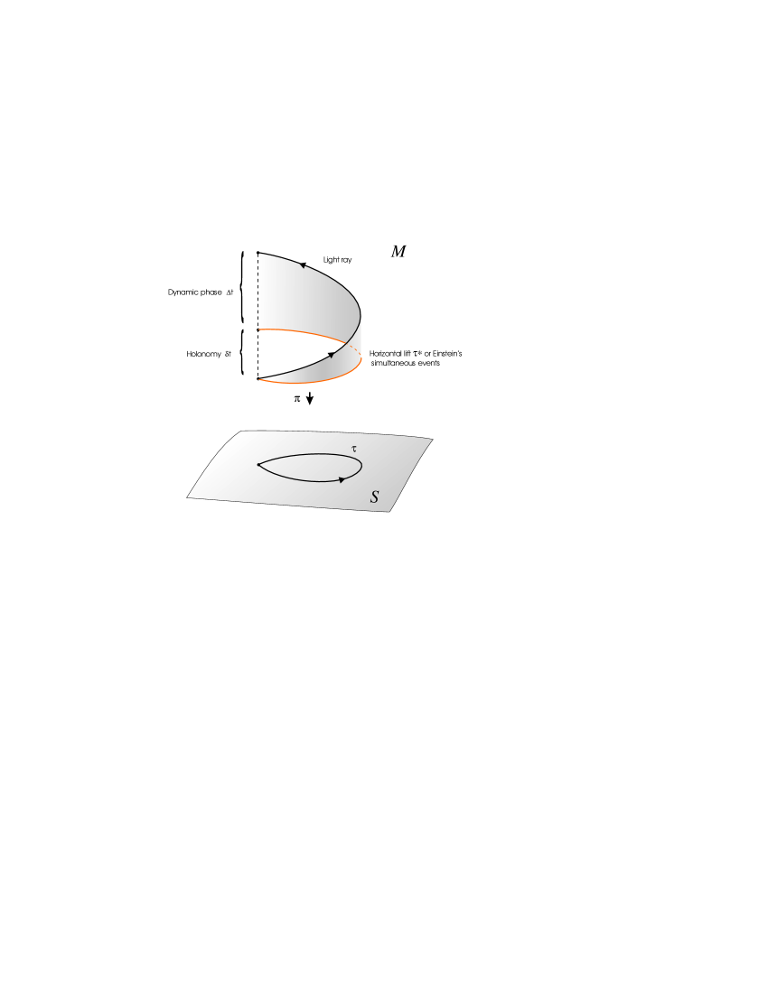
Figure 2: The horizontal lift and its relation with the pointwise Einstein synchronization.

Before we start studying the curvature and its implications, we recall some notions regarding local observers. An observer is identified by a tetrad of orthonormal vectors $\{u,e_{1},e_{2},e_{3}\}$. A picture of $e_{i}$ may be the following: imagine the local laboratory of the observer to be a cube. The observer, at rest in the cube, stands by one of the corners and the normal vectors $e_{i}$ point towards the next three corners. Since $e_{i}$ points always towards the same corner it must satisfy

$$L_{k}\,e_{i}=0.$$ (6)

Let $h^{\mu}_{\nu}=\delta^{\mu}_{\nu}-u^{\mu}u_{\nu}$ be the projector on the horizontal space of the observer. The evolution of the components of $e_{i}$ with respect to a Fermi transported tetrad (non-rotating reference frame) $\hat{e}_{\mu}$ is well known hawking73 , the relevant quantities are the vorticity tensor

$$w_{\mu\nu}=h^{\alpha}_{\mu}h^{\beta}_{\nu}\,u_{[\alpha;\,\beta]}\,,$$ (7)

which represents the angular velocity of the triad $e_{i}$ with respect to gyroscopes ($\hat{e}_{i}$), and the expansion tensor

$$\theta_{\mu\nu}=h^{\alpha}_{\mu}h^{\beta}_{\nu}\,u_{(\alpha;\,\beta)}\,,$$ (8)

which represents the rate of separation of neighboring points from the worldline. From Eq. (1), after some algebra, we find that the expansion tensor vanishes thus allowing a local rigidity interpretation. The vorticity can be rewritten

$$w_{\mu\nu}=\sqrt{k\cdot k}\,\,\omega_{[\mu;\,\nu]}=-\frac{\sqrt{k\cdot k}}{2}\,\Omega_{\mu\nu},$$ (9)

where we have introduced the curvature

$$\Omega=D\omega=({\rm d}\omega)h={\rm d}\omega.$$ (10)

The translational invariance of spacetime implies that the vorticity, the curvature and the norm of the Killing vector field have a vanishing Lie derivative. As a consequence the angular velocity of an observer at rest in the stationary frame points always in the same direction with the same norm. Its components with respect to $e_{i}$ do not change in time.

Gauge theory tells us that if $S$ is paracompact and simply connected the curvature vanishes if and only if the horizontal lifts of closed curves in $S$ are closed in $M$. In order to make use of the Einstein convention the horizontal lift should be closed, otherwise there would be two simultaneous events placed in the same time-like worldline. In that case, the Einstein convention would be of little use. If the topological requirements are satisfied: the Einstein synchronization convention is applicable if and only if, in every point of the stationary frame, observers at rest do not rotate godel49 . Moreover, if the vorticity is different from zero in a point $s$ of space, an observer at rest in that point feels inertial forces because its local reference frame rotates with respect to Fermi transported gyroscopes. These observations assure that the rotating platform in special relativity is indeed quite representative of the general interrelationship between the Einstein convention, inertial forces, and rotation.

Let us study the simple case $\Omega=0$. Gauge theory tells us that, when the curvature vanishes, there exists a foliation of the principal bundle in three-dimensional hypersurfaces with horizontal tangent spaces. They are the hypersurfaces of simultaneity accordingly with the Einstein convention. Those hypersurfaces are orthogonal to the Killing vector field because their tangent spaces are also orthogonal to it. The existence of hypersurfaces orthogonal to a vector field is the object of Frobenius theorem: the necessary and sufficient condition for the vector field $v^{\mu}$ to be hypersurface orthogonal is $v_{[\alpha}\nabla_{\beta}v_{\gamma]}=0$. This condition is indeed coherent with $\Omega=0$ because the equations

$$\Omega = 0,$$ (11)

$$k\wedge{\rm d}k = 0,$$ (12)

are algebraically the same.

If $\Omega\neq 0$ the Einstein convention is no longer applicable. Here gauge theory suggests a standard procedure to extend coordinates $\{x^{i}\}$ on $S$ to the whole principal bundle. First choose a section $\sigma:S\rightarrow M$ and then associate to the event $\sigma(x^{i})e^{t}$ the coordinates $\{x^{i},t\}$. This procedure depends on the section (gauge) chosen and, from the physical side, corresponds to taking the events on the hypersurface $\sigma(S)$ as simultaneous. A number of different simultaneity conventions can be adopted, each one in correspondence with a particular section. In geometry the change of section is exactly what in physics is a gauge transformation. Hence we pass from one convention to another via gauge transformations. Usually in physics one works with the potential, that is with the pullback $A_{\sigma}(x^{i})=\sigma^{*}\omega$. In the coordinates $\{x^{i},t\}$, the Poincaré connection becomes

$$\omega={\rm d}t+A_{\sigma}(x^{i}).$$ (13)

It is invariant under the change of section (gauge transformation)

$$t^{\prime} = t-\alpha(x^{i}),$$ (14)

$$A_{\sigma^{\prime}} = A_{\sigma}+{\rm d}\alpha(x^{i}).$$ (15)

It is also convenient to introduce the field strength $F(x^{i})=\sigma^{*}\Omega={\rm d}A_{\sigma}$. Let us come to a frequent question in gauge theories. If $\tau(\lambda):[0,1]\rightarrow S$ is a closed curve, how much is $\delta t$ such that $\tau^{*}(1)=\tau^{*}(0)e^{\delta t}$? In order to answer this question we have to recall that $\tau^{*}$ has horizontal tangent vectors. Integrating $\omega$ over $\tau^{*}$ we find

$$\delta t=-\oint_{\tau}A_{\sigma}.$$ (16)

The physical interpretation of this result is connected with the Sagnac effect sagnac13 ; anandan81 .

III Space metric and Sagnac effect

Let us define over $S$ a metric through the formula moller62 ; gron77 ; landau62 ; weber97

$${\rm d}l^{2}=-h_{ij}{\rm d}x^{i}{\rm d}x^{j}\qquad i,j=1,2,3$$ (17)

in the coordinates $\{x^{i},t\}$ introduced above. From a geometrical perspective this formula for the space metric ${\rm d}l^{2}$ can be rewritten

$${\rm d}l^{2}(X,Y)=-g(X^{*},Y^{*})\,,$$ (18)

where $X^{*}$, $Y^{*}$, are the horizontal lifts of the space vectors $X$, $Y$. The vectors $X^{*}$, $Y^{*}$ belong to the horizontal space of the observer which passes through their origin, and that horizontal space is nothing but the local space of an inertial observer. Hence, from a physical point of view the previous formula says that the space metric is induced from the measurements made by local inertial observers. This statement relies on the fact that, for an inertial observer, the spacetime metric serves also to define the space metric through the formula $\eta(X^{*},Y^{*})$ where $X^{*}$, $Y^{*}$ belong to its space. However it is an assumption that for accelerating or rotating observers, space measurements should coincide with those performed by inertial observers. This postulate referred also as the ”surrogate frames postulate” klauber98 is waiting an experimental verification. Actually, in our stationary frame, observers at rest in the frame are not necessarily inertial. To claim that equation (18) describes accurately the space metric as experimented by observers at rest in the frame, would go beyond our knowledge. A number of alternatives, especially for the rotating platform have been suggested strauss74 ; klauber98 . A similar debate raised in the contest of Kaluza-Klein extensions of gravity where two different interpretations of the five dimensional metric were natural: those of Weyl and Pauli overduin97 . This is not accidental as the mathematics involved in the spacetime splitting in time plus space is that of Kaluza -Klein theories. Indeed the spacetime metric can be rewritten

$$g(A,B)=(k\cdot k)\omega(A)\omega(B)-{\rm d}l^{2}(\pi_{*}A,\pi_{*}B)\,,$$ (19)

which is a Kaluza-Klein metric in the spacetime manifold. Another useful choice for the space metric is the optical metric abramowicz88 , ${\rm d}\bar{l}={\rm d}l/(k\cdot k)$. Indeed the geodesics of light, and hence their projections, are invariant under conformal transformations of the spacetime metric $g$. In the study of light propagation we can reduce the spacetime metric to the form, ${\rm d}\bar{s}^{2}=\omega^{2}-{\rm d}\bar{l}^{2}$ where no conformal factor appears. Now, the projection of a geodesic of a Kaluza-Klein metric with unitary scalar field, $k\cdot k=1$, satisfies a straightforward generalization of the Lorentz law. In the null case it reads

$$\bar{\nabla}_{v}v^{i}=F^{i}_{j}v^{j}\,,$$ (20)

where $v^{i}={\rm d}x^{i}/{\rm d}\bar{l}$ is the tangent vector of the projection and $\bar{\nabla}$ is the covariant derivative with respect to the optical Levi-Civita connection. Hence, at least light rays, satisfy a Lorentz like equation in the optical metric background. Here we use the optical metric as a tool for finding the dynamic phase(see figure 2).

Let us consider two light beams that leave $\tau^{*}(0)$ following the path $\tau(\lambda)$, one in the positive direction and the other in the negative direction. Figure 2 shows one of the beam and displays some relevant quantities like the dynamic phase $\Delta t$ and the holonomy $\delta t$. As seen from the local inertial frames along $\tau$, with respect to their local Einstein synchronized times, the two light beams have the same speed $c=1$. Let $l$ be the natural parameter of $\tau$. The dynamic phase is

$$\Delta t=\int_{\tau^{*}}{\rm d}t=\int_{\tau^{*}}\frac{{\rm d}\tau}{\sqrt{k\cdot k}}=\oint_{\tau}\frac{{\rm d}l}{c\sqrt{k(l)\cdot k(l)}}=\bar{L}/c\,.$$ (21)

Where $\bar{L}$ is the total optical length of the path $\tau$. Coming back to the Sagnac effect, the dynamic phase does not depend on the direction followed by the light beam. On the contrary, the holonomy changes sign; as a consequence the difference of the arrival times of the two beams is twice Eq. (16), and taking into account the time dilation, that is the difference between Killing time and proper time, the Sagnac effect becomes

$$\delta\tau=-2\sqrt{k\cdot k}\oint_{\tau}A_{\sigma}\,.$$ (22)

This equation is conveniently written in the coordinates $\{x^{i},x^{0}=t\}$. Let $\Sigma$ be a two-dimensional surface such that $\tau=\partial\Sigma$. From $k=\partial_{t}$ we have $k_{\mu}=g_{\mu\nu}k^{\nu}=g_{\mu 0}$ and $A_{\sigma i}=g_{0i}/g_{00}$, hence ashtekar75

$$\delta\tau=-2(g_{00})^{\frac{1}{2}}\oint_{\tau}\frac{g_{0i}}{g_{00}}\,{\rm d}x^{i}=2(g_{00})^{\frac{1}{2}}\int_{\Sigma}\frac{w_{ij}}{(g_{00})^{\frac{1}{2}}}\,{\rm d}x^{i}\wedge{\rm d}x^{j}\,.$$ (23)

Notice that the worldline of a point at rest in the stationary frame has equation, $x^{i}=const.$. This condition, and the independence of $g_{\mu\nu}$ of time, selects those systems of coordinates for which the previous equation holds.

We have completed our exposition of the gauge property of simultaneity in stationary frames. The reader familiar with gauge theories can easily recognize the formal similarity with electrodynamics. Both theories have the mathematical structure of a gauge theory over a one-dimensional group. The only relevant difference is that in the stationary frame the structure group is contractible (otherwise there would be closed time-like curves), whereas in electrodynamics, $U(1)$, is not. This implies that, in electrodynamics, we can have non trivial principal bundles like monopoles, whereas this is not possible in the present context. Other analogies, like that between the Sagnac effect and the Aharonov-Bohm effect sakurai80 , or like that between magnetic forces and Coriolis forces coisson73 ; semon81 , become self evident in light of the gauge interpretation.

Gauge theory	Simultaneity
Fiber bundle	Spacetime manifold
$P$	$M$
Structure group	Group of time translations
$G$	$T_{1}$
Base	Space of worldlines
	$S$
Fiber	Worldline of an observer
	at rest in the frame
Vertical space at	Space spanned by the four
the point $p$	velocity of an observer at $p$
Horizontal space	Local Einstein’s
	simultaneous events
Horizontal lift	Pointwise Einstein’s
	synchronization
Connection	Poincaré connection $P$
Choice of the section	Choice of the simultaneity
	convention
Gauge transformation	Change of the simultaneity
	convention
Curvature	Angular velocity of observers
	at rest in the frame
Bianchi identity	$Dw+a\wedge w=0$
Holonomy	Sagnac effect
Dynamic phase	Optical round trip time
	in absence of holonomy
	$\bar{L}/c$
Kaluza-Klein metric	Spacetime metric

Table 1: Gauge interpretation of simultaneity. The correspondences in italic hold in stationary frames but do not hold in general.

IV Simultaneity in non-stationary frames

So far we have considered stationary frames. In general, however, the trajectories of the observers which define the frame, are not generated by a Killing vector field. This does not imply that the simultaneity is no more described by a gauge theory, but only that there is no connection preserving structure group. We can still define the space $S$ as the manifold of the observer worldlines. Then, discarding some pathological choices for the trajectories, at least in an open set, the space $S$ will be a differentiable manifold and there will be a differentiable projection $\pi:M\rightarrow S$. Hence, again, $M$ can be considered as a fiber bundle over the space $S$.

It should be noticed that over this bundle one can define the action of the one-parameter group of diffeomorphisms $\phi^{u}_{\tau}$ generated by the four-velocity field $u(x)$. With this right action $M$ can be considered, at least locally, as a principal bundle. However, in general, such a structure group does not preserve the simultaneity connection. It is, then, more convenient to treat $M$ as a fiber bundle without structure group since the beginning.

The theory of connections, i.e. gauge theory, was developed by mathematicians in this general context michor91 . Generalized connections appeared also in physics in some works on Kaluza-Klein theory and general relativity cho92 ; Yoon99 . In those papers it was shown that most of the usual gauge theory has an analogue in the new setting even from the dynamical side. However, they did not take advantage of the coordinate-independent approach developed by mathematicians.

Let us introduce the generalized connection in a form useful for our purposes. A connection is given by a distribution of planes $H_{x}$, that is, by a differentiable assignment, in each point of the bundle, of a plane that we shall call horizontal. The plane, together with the tangent space of the fiber spans the tangent space at $x$. The relevant difference with the usual gauge theory is the absence of a structure group which sends the fiber to itself and horizontal planes to horizontal planes. Many of the features of the usual gauge theory have a generalization. It is still possible to define the horizontal lift, the curvature and the parallel transport. Even the Bianchi identities have a generalization michor91 .

In our case, the fiber bundle M has a natural connection. The horizontal planes are given by $H_{x}=\text{ker}(u_{\alpha}(x){\rm d}x^{\alpha})$ where $u^{\alpha}$ is the four-velocity of the observer. In this way the connection maintains its original meaning: the horizontal plane still selects, locally, those events which are simultaneous accordantly with the Einstein synchronization convention. Analogously, the horizontal lift $\tau^{*}$ is obtained by a pointwise Einstein synchronization over $\tau$. Notice that the connection $\omega=u_{\alpha}{\rm d}x^{\alpha}$ is defined only up to a spacetime factor, because its ker does not change after such a multiplication. For this reason, in the generalized gauge theory, one works with the vector valued connection $P^{\beta}_{\alpha}=u^{\beta}u_{\alpha}$, which is the projector of the tangent space onto the vertical subspace. The curvature is defined through the Frölicher-Nijenhuis bracket which acts on a pair of vector valued forms, say $K$ and $L$ of degree $k$ and $l$ respectively, giving a vector valued form of degree $k+l$. If $K=\alpha\otimes z$ and $L=\beta\otimes v$ with $z$ and $v$ vector fields, the Frölicher-Nijenhuis bracket can be characterized by

$$[\alpha\otimes z \beta\otimes v]_{FN}=\alpha\wedge\beta\otimes[z,v]+\alpha\wedge L_{z}\beta\otimes v$$ ,

$$\ \ \ -(-1)^{kl}\beta\wedge L_{v}\alpha\otimes z+(-1)^{k}i_{v}\alpha\wedge d\beta\otimes z$$

$$\ \ \ -(-1)^{kl+l}i_{z}\beta\wedge d\alpha\otimes v,$$

where $[\,,]$ is the Lie-bracket.

The vector valued curvature $R$ (which has nothing to do with the Riemann tensor), and its real counterpart $\Omega$ are defined through the formula

$$2R=-[P,P]_{FN}\qquad\text{or}\qquad 2u^{\beta}\Omega=-[u^{\mu}\omega,u^{\nu}\omega]_{FN}.$$ (24)

After some algebra the previous equation reads

$$\Omega=D\omega\,,$$ (25)

that is, the same expression obtained for the usual gauge theory. This expression is invariant under multiplication of the connection and the curvature by the same factor $f(x)$. Previously that factor was fixed by the requirement $\omega(k)=1$. Here it is fixed by $\omega(u)=1$. In this normalization the curvature is linked to the vorticity through the relation $\Omega_{\mu\nu}=-2w_{\mu\nu}$.

Let $A=\partial/\partial a$, $B=\partial/\partial b$, be two fields over $S$ of vanishing Lie bracket, and let $A^{*}$ and $B^{*}$ be their horizontal lift. Plugging these fields in Eq. (25) we find

$$[A^{*}\Delta a,B^{*}\Delta b]^{\mu}u_{\mu}=2w_{\alpha\beta}\,A^{*\alpha}\Delta a\,B^{*\beta}\Delta b\,.$$ (26)

The left hand side expresses the holonomy of a closed path $\tau$ of sides $\Delta x^{i}=A^{i}\Delta a$ and $\Delta x^{i}=B^{i}\Delta b$ in units of proper time. That is, it gives half the Sagnac effect for the path described. The right hand side stands for the product $2\vec{\omega}\cdot\vec{\Delta S}$ where $\vec{\Delta S}$ is the oriented area enclosed by the path $\tau$. Hence, Eq. (26) is an infinitesimal, and general relativistic version of the well known formula of the Sagnac effect stedman97

$$\delta\tau=\frac{4\vec{\omega}\cdot\vec{\Delta S}}{c^{2}}\,.$$ (27)

Notice that this equation holds only for infinitesimal paths. In the case of a stationary frame, there is an integral version given by Eq. (23).

In the generalized gauge theory the Bianchi identity reads

$$[P,R]_{FN}=0\,.$$ (28)

After some calculations, and using only the horizontality of the 2-form $\Omega$ one arrives at

$$D\Omega+a\wedge\Omega=0\,.$$ (29)

Hence, the Bianchi identity is a non trivial, and quite unexpected, differential relation between the vorticity and the acceleration field. In terms of the vorticity vector

$$w^{\alpha}=\frac{1}{2}\,\varepsilon^{\alpha\beta\gamma\delta}u_{\beta}w_{\gamma\delta}\qquad;\qquad w_{\alpha\beta}=\varepsilon_{\alpha\beta\gamma\delta}u^{\gamma}w^{\delta},$$ (30)

the Bianchi identity takes the form

$$w^{\nu}_{;\,\nu}+2w^{\nu}a_{\nu}=0.$$ (31)

This identity can be checked directly using Eq. (7) and Eq. (30). The physical meaning follows recalling that in flat spacetime and for a non-relativistic fluid described by a vector field $\vec{v}$ the vorticity vector is $\vec{\omega}=\frac{1}{2}\nabla\times\vec{v}$. Thus in the non-relativistic limit $\nabla\cdot\vec{\omega}=0$. The Bianchi identity is therefore a generalization of this equation to the relativistic case. It shows that when relativistic effects are taken into account the acceleration becomes a source for the vorticity vector. Restoring $c$ one sees that this effect, in the non-relativistic limit, is suppressed by a factor $1/c^{2}$.

Table 1 summarizes the parallelism between simultaneity and gauge theory.

V Back to the usual gauge theory

One can ask what is the condition that the vector field $u$ should satisfy in order for the connection to be principal. In other words, in what circumstance is there a vector field

$$X=\chi(x)u\,,$$ (32)

whose one parameter group of diffeomorphisms $\phi^{X}_{t}$ with $X=\partial_{t}$ sends horizontal planes to horizontal planes? If it exists one can choose

$$\omega_{\mu}=\frac{X_{\mu}}{X\cdot X}\,,$$ (33)

and Eqs. (3) and (4) become both satisfied. The invariance of the horizontal planes under the group of diffeomorphisms $\phi^{X}_{t}$ reads

$$\phi^{X}_{t\,*}\,H_{x}=H_{\phi^{X}_{t}(x)}\,.$$ (34)

Let $\omega$ be a real valued connection ($\text{ker}\,\omega(x)=H_{x}$). The previous equation becomes

$$L_{X}\omega=f(x)\omega\,,$$ (35)

for a suitable function $f:M\to\mathbb{R}$. Let us begin with $\omega_{\beta}=X_{\beta}$, we find

$$(L_{X}\,g)_{\beta\nu}X^{\nu}=fX_{\beta}\,.$$ (36)

This equation is equivalent to Eq. (34). It is satisfied, for instance, if $X$ is a conformal Killing vector field

$$L_{X}g=\frac{X^{\mu}_{;\mu}}{2}\,g\,,$$ (37)

hence our previous treatment of simultaneity in stationary frames can be easily generalized to conformal stationary frames. In both cases the connection is principal, that is, invariant under the action of a structure group. This should have been expected because the relation of orthogonality follows solely from the causal structure of spacetime, that is, it is invariant under conformal transformations of the metric. A conformal Killing vector field, preserving the causal structure, preserves also the orthogonality relation and therefore sends horizontal planes to horizontal planes. Equation (36), however, does not solve our problem because it is not expressed in terms of the four-velocity field $u(x)$.

Let $\omega_{\beta}=u_{\beta}$, plugging this equation in Eq. (35) we find after some algebra

$$\nabla_{u}u_{\beta}+(\ln\chi)_{\beta}=u_{\beta}\nabla_{u}(\ln\chi)\,.$$ (38)

The projection of this equation to the vertical space is automatically satisfied. It is convenient to introduce the acceleration 1-form $a_{\beta}=\nabla_{u}u_{\beta}$ and to project the previous equation to the horizontal plane

$$D(\ln\chi)=-a\,.$$ (39)

The problem is solved if we can establish in what circumstances this equation has a solution $\ln\chi$ ($\chi^{-1}$ is the acceleration potential ellis71 ) over the fiber bundle). The condition we are seeking is an integrability condition for Eq. (39). It should be noticed that Eq. (39) gives us the value of $\partial_{Y}(\ln\chi)$ only for $Y\in H_{x}$. In order to find $\partial_{u}(\ln\chi)$ we have to use the non integrability of the distribution of horizontal planes. If $R=0$, however, the distribution of horizontal planes becomes integrable and the spacetime admits a foliation of simultaneity slices. In that case there is an infinite number of solutions (if any), each one in correspondence with a different time parameterization of the simultaneity slices. The equivalence relation ”$x\sim y$ if there exists a piecewise $C^{1}$ horizontal curve which joins $x$ and $y$”, divides the spacetime manifold into sets $M_{i}$, $M=\cup_{i}M_{i}$. In each set the equation (39) has a unique solution $\chi(x)$ up to a constant factor. Indeed if $\chi^{\prime}$ is another solution of Eq. (39) then $D\ln(\chi{\chi^{\prime}}^{-1})=0$ and hence $\chi{\chi^{\prime}}^{-1}=c_{i}$ in each set $M_{i}$ .

Without losing generality we can restrict ourselves to a region $M_{i}$ where each pair of events can be joined by a horizontal curve. We assume that $M_{i}$ is simply connected. Let us consider the 1-form

$$\sigma=f(x)u-a\,,$$ (40)

where $f(x)$ is a real valued function. With a straightforward calculation it is easy to show that ${\rm d}\sigma=0$ if and only if

$$Da = f\,Du\,,$$ (41)

$$L_{u}a = f\,a-Df\,.$$ (42)

In this case, $\sigma={\rm d}\varphi$ and from Eq. (40), $f=\partial_{u}\varphi$ and $D\varphi=-a$. Since $\varphi$ solves Eq. (39) it is the function $\ln\chi$ we are looking for. Conversely if $\ln\chi$, solution of (39), exists, it satisfies Eqs. (40-42) with $f=\partial_{u}\ln\chi$.

The system of equations (41) (42) is our necessary and sufficient condition in order to establish whether our connection is principal. The first equation (41) states that the two forms $Da$, $Du$ must be proportional: the proportionality factor gives the derivative $f=\partial_{u}(\ln\chi)$ that Eq. (39) was unable to determine. The second equation (42) states a condition that can be checked once we substitute $f(x)$ as given by Eq. (41). Hence, we can establish whether or not the simultaneity is described by a principal connection looking only at the physical data $u(x)$.

If $a=0$ the system is solvable with the solution $\chi(x)=1$. This result says that, when the congruence of time-like curves is given by geodesics, the simultaneity can be treated as a gauge theory over the group of time translations.

Another interesting case, which generalizes the previous one, is that of a perfect fluid of equation of state $p=p(\rho)$. The stress-energy tensor is

$$T^{\mu\nu}=(\rho+p)u^{\mu}u^{\nu}-p\,g^{\mu\nu},$$ (43)

The conservation of 4-momentum $T^{\mu\nu}_{;\nu}$ leads to the local energy conservation and to the Euler equation

$$\rho_{,\,u} = -(\rho+p)\nabla\cdot u$$ (44)

$$(\rho+p)\,a = Dp$$ (45)

One can introduce the functions ellis71

$$\chi = \exp\left(-\int_{p_{0}}^{p}\frac{{\rm d}p}{\rho+p}\right)$$ (46)

$$R = \exp\left(-\int_{\rho_{0}}^{\rho}\frac{{\rm d}\rho}{3(\rho+p)}\right)=\chi^{-1/3}\left(\frac{\rho+p}{\rho_{0}+p_{0}}\right)^{-1/3}$$ (47)

which are related to each other and to the pressure. Using the relation between the determinants $g=\chi^{2}h$, the energy-momentum conservation becomes

$$\left(\ln(R^{-3}|h|^{\frac{1}{2}})\right)_{,u} = 0$$ (48)

$$a+D\ln\chi = 0$$ (49)

This last equation says that the flow lines of the perfect fluid define a frame where the simultaneity is described by a gauge theory over the group of time translation. The invariance of the connection $\omega$ under time translations (see Eq. (4) and Eq. (13)) implies that the potential $A_{\sigma}$ does not depend on time. Making use of Eqs. (48) (19) (13) and introducing $\bar{h}_{ij}=R^{-2}h_{ij}$, the spacetime metric becomes

$$g_{\mu\nu}{\rm d}x^{\mu}{\rm d}x^{\nu}\!=\!\chi(x)^{2}({\rm d}t+A_{i}(x^{j}){\rm d}x^{i})^{2}\!+\!R(x)^{2}\bar{h}_{ij}(x^{k},t){\rm d}x^{i}\!{\rm d}x^{j}$$

where the determinant $\bar{h}$ does not depend on time. The function $R(x)$ can be interpreted as the scale factor of the universe since a volume element scales as $R^{3}$ with time ($\theta=\nabla\cdot u=3R_{,\,u}/R$). This well known result, already obtained by Ehlers, Taub and others (see ellis71 and references therein) arises here as a natural consequence of a careful analysis of simultaneity in the simple case of a perfect fluid with an acceleration potential.

VI Conclusions

I have shown that simultaneity is described by the mathematics of gauge theories. The fiber bundle is the spacetime manifold and the fibers are the trajectories which define the frame. The connection is determined by local simultaneous events accordantly with the Einstein convention, and the horizontal lift follows from a pointwise Einstein synchronization. The curvature is the angular velocity of the observers at rest in the frame and the holonomy is the obstruction against the possibility of applying the Einstein synchronization in the large. A global simultaneity convention allows the introduction of a time coordinate on the manifold. A change in the global simultaneity convention is a gauge transformation. The gauge formalism suggested the calculation of the Bianchi identity which turned out to be a differential relation between the acceleration field and the vorticity field.

A necessary and sufficient condition on the vector field $u(x)$ in order for the connection to be principal has been given. In that case the fiber bundle admits a structure group $T_{1}$ of time translations which preserves the connection, and the usual gauge theory is recovered. Particular cases are frames of geodesics, frames derived from the flow lines of a perfect fluid and conformal stationary frames. In this last case the Sagnac effect depends straightforwardly on the holonomy of the light path through a generalization of Eq. (23). Apart from these simple cases, in order to appreciate the gauge nature of simultaneity, in the spirit of contemporary physics, the whole machinery of the Frölicher-Nijenhuis algebra is needed.

The gauge picture of simultaneity is expected to be useful in the search for non trivial solutions of the Einstein equations. Moreover, once generalized to higher dimensions, the mathematics involved can prove to be useful in modern Kaluza-Klein theories, since there, the cylinder condition is dropped.

References

- (1) M. A. Abramowicz, B. Carter, and J.P. Lasota. Optical reference geometry for stationary and static dynamics. Gen. Relativ. Gravit., 20:1173–1183, 1988.
- (2) J. Anandan. Sagnac effect in relativistic and non-relativistic physics. Phys. Rev. D, 24:338–346, 1981.
- (3) R. Anderson, I. Vetharaniam, and G. E. Stedman. Conventionality of synchronization, gauge dependence and test theories of relativity. Phys. Rep., 295:93–180, 1998.
- (4) S. J. R. Anderson and G. E. Stedman. Distance and the conventionality of simultaneity in special relativity. Found. Phys. Lett., 5:199–220, 1992.
- (5) A. Ashtekar and A. Magnon. The Sagnac effect in general relativity. J. Math. Phys., 16:341–344, 1975.
- (6) Y. M. Cho, K. S. Soh, J. H. Yoon, and Q.-H. Park. Gravitation as a gauge theory of the diffeomorphism group. Physics Letters B, 286:251–255, 1992.
- (7) R. Coisson. On the vector potential of Coriolis forces. Am. J. Phys., 41:585–586, 1973.
- (8) G.F.R. Ellis. Isotropic solutions of the Einstein-Boltzmann equations. Commun. Math. Phys., 23:1–22, 1971.
- (9) K. Gödel. An example of a new type of cosmological solutions of Einstein’s field equations of gravitation. Rev. Mod. Phys., 21:447–50, 1949.
- (10) Ø. Grøn. Rotating frames in special relativity analyzed in light of a recent article by M. Strauss. Int. J. Theor. Phys., 16:603–614, 1977.
- (11) S. W. Hawking and G. F. R. Ellis. The Large Scale Structure of Space-Time. Cambridge University Press, Cambridge, 1973.
- (12) R. Klauber. New perspectives on the relativistically rotating disk and non-time-orthogonal reference frames. Found. Phys. Lett., 11:405–443, 1998.
- (13) S. Kobayashi and K. Nomizu. Foundations of Differential Geometry, volume I of Interscience tracts in pure and applied mathematics. Interscience Publishers, New York, 1963.
- (14) L. D. Landau and E. M. Lifshitz. The Classical Theory of Fields. Addison-Wesley Publishing Company, Reading, 1962.
- (15) D. Malament. Causal theories of time and the conventionality of simultaneity. Noûs, 11:293–300, 1977.
- (16) L. Mangiarotti and M. Modugno. Graded Lie algebras and connections on a fibered space. J. Math pures et appl., 63:111–120, 1984.
- (17) R. F. Märzke and J. A. Wheeler. in: Gravitation and Relativity. Benjamin, New York, H.-Y. Chiu and W.F. Hoffmann edition, 1964. p. 40.
- (18) P. W. Michor. Gauge theory for fiber bundles, volume 19 of Monographs and Textbooks in Physical Sciences. Bibliopolis, Napoli, 1991.
- (19) E. Minguzzi. On the conventionality of simultaneity. Found. Phys. Lett., 15:153–169, 2002.
- (20) E. Minguzzi and A. Macdonald. Universal one-way light speed from a universal light speed over closed paths. gr-qc/0211091, 2002.
- (21) M. Modugno. Torsion and Ricci tensor for non-linear connections. Differential Geometry and its Application, 1:177–192, 1991.
- (22) C. Møller. The Theory of Relativity. Clarendon-Press, Oxford, 1962.
- (23) J. M. Overduin and P. S. Wesson. Kaluza-Klein gravity. Phys. Rep., 283:303–378, 1997.
- (24) M. Pauri and M. Vallisneri. Märzke-Wheeler coordinates for accelerated observers in special relativity. Found. Phys. Lett., 13:401–425, 2000.
- (25) H. Poincaré. Bull. des Sci. Math., 28:302, 1904.
- (26) H. Poincaré. La Revue des Idées, 1:801, 1904.
- (27) A. A. Robb. A Theory of Time and Space. Cambridge University Press, Cambridge, 1914.
- (28) M. G. Sagnac. C. R. Acad. Sci., 157:708, 1913. ibid. 1410.
- (29) J. J. Sakurai. Comments on quantum-mechanical interference due to the Earth’s rotation. Phys. Rev. D, 21:2993–2994, 1980.
- (30) M. D. Semon and G. M. Schmieg. Note on the analogy between inertial and electromagnetic forces. Am. J. Phys., 49:689–690, 1981.
- (31) G. E. Stedman. Ring-laser tests of fundamental physics and geophysics. Rep. Prog. Phys., 60:615–688, 1997.
- (32) N. Steenrod. The Topology of Fibre Bundles. Princeton University Press, Princeton, 1970.
- (33) M. Strauss. Rotating frames in special relativity. Int. J. Theor. Phys., 11:107–123, 1974.
- (34) T. A. Weber. Measurements on a rotating frame in relativity, and the Wilson and Wilson experiment. Am. J. Phys., 65:946–953, 1997.
- (35) C. M. Will. Clock synchronization and isotropy of the one-way speed of light. Phys. Rev. D, 45:403–411, 1992.
- (36) T. T. Wu and C. N. Yang. Concept of nonintegrable phase factors and global formulation of gauge fields. Phys. Rev. D, 12:3845–3857, 1975.
- (37) J. H. Yoon. Kaluza-Klein formalism of general spacetimes. Physics Letters B, 451:296–302, 1999.