Braneworld Dynamics of Inflationary Cosmologies with Exponential Potentials

Abstract

In this work we consider Randall - Sundrum brane - world type scenarios, in which the spacetime is described by a five - dimensional manifold with matter fields confined in a domain wall or three-brane. We present the results of a systematic analysis, using dynamical systems techniques, of the qualitative behaviour of Friedmann - Lemaître - Robertson - Walker type models, whose matter is described by a scalar field with an exponential potential. We construct the state spaces for these models and discuss how their structure changes with respect to the general - relativistic case, in particular, what new critical points appear and their nature and the occurrence of bifurcation.

I Introduction

String and membrane theories are considered to be promising candidates for a unified theory of all forces and particles in Nature. Since a consistent construction of a quantum string theory is only possible in more than four spacetime dimensions we are compelled to compactify any extra spatial dimensions to a finite size or, alternatively, find a mechanism to localize matter fields and gravity in a lower dimensional submanifold.

Motivated by orbifold compactification of higher dimensional string theories in particular the dimensional reduction of eleven - dimensional supergravity introduced by Ho$\check{\mbox{r}}$ava and Witten Horava1 ; Horava2 , Randall and Sundrum showed that for non - factorisable geometries in five dimensions there exists a single massless bound state confined in a domain wall or three - brane Randall . This bound state is the zero mode of the Kaluza - Klein dimensional reduction and corresponds to the four - dimensional graviton. This scenario may be described by a model consisting of a five - dimensional Anti - de Sitter space (known as the bulk) with an embedded three - brane on which matter fields are confined and Newtonian gravity is effectively reproduced on large - scales. A discussion of earlier work on Kaluza - Klein dimensional reduction and matter localization in a four - dimensional manifold of a higher - dimensional non - compact spacetime can be found in List1 .

Gravity on the brane can be described by the standard Einstein equations modified by two additional terms, one quadratic in the energy - momentum tensor and the other representing the electric part of the five - dimensional Weyl tensor.

Following an approach to the study of homogeneous cosmological models with a cosmological constant first introduced by by Goliath and Ellis Goliath (see also Dynamics for a detailed discussion of the dynamical systems approach to cosmology), Campus and Sopuerta have recently studied the complete dynamics of Friedmann - Lemaître - Robertson - Walker (FLRW) and the Bianchi type I and V cosmological models with a barotropic equation of state, taking into account effects produced by the corrections to the Einstein Field Equations Campos .

Their analysis led to the discovery of new critical points corresponding to the Bin$\acute{\mbox{e}}$truy - Deffayet - Langlois (BDL) models Binetruy , representing the dynamics at very high energies, where effects due to the extra dimension become dominant. These solutions appear to be a generic feature of the state space of more general cosmological models. They also showed that the state space contains new bifurcations, demonstrating how the dynamical character of some of the critical points changes relative to the general - relativistic case. Finally, they showed that for models satisfying all the ordinary energy conditions and causality requirements the anisotropy is negligible near the initial singularity, a result first demonstrated by Maartens et. al. Maartens-Sahni .

In this paper we extend their work to the case where the matter is described by a dynamical scalar field $\phi$ with an exponential potential $V(\phi)=\exp(b\phi)$. This work builds on earlier results obtained by Burd and Barrow Burd and Haliwell Halliwell who considered the dynamics of these models in standard general relativity (GR). Van den Hoogen et. al. and Copeland et. al. have also considered the GR dynamics of exponential potentials in the context of Scaling Solutions in FLRW spacetimes containing an additional barotropic perfect fluid Hoogen ; Copeland .

It is worth mentioning that Exponential potentials are somewhat more interesting in the brane - world scenario, since the high - energy corrections to the Friedmann equation allow for inflation to take place with potentials ordinarily too steep to sustain inflation Copeland2 .

II Preliminaries

In what follows we summarise the geometric framework used analyse the brane - world scenario in the cosmological context.

II.1 Basic equations of the brane - world

In Randall - Sundrum brane - world type scenarios matter fields are confined in a three - brane embedded in a five - dimensional spacetime (bulk). It is assumed that the metric of this spacetime, $g^{(5)}_{AB}$, obeys the Einstein equations with a negative cosmological constant $\Lambda_{(5)}$ Shiromizu ; Sasaki ; Maartens )

$$G^{(5)}_{AB}=-\Lambda_{(5)}g^{(5)}_{AB}+\kappa^{2}_{(5)}\delta(\chi)\left[-\lambda\,g_{AB}+T_{AB}\right]\;,$$ (1)

where $G^{(5)}_{AB}$ is the Einstein tensor, $\kappa_{(5)}$ denotes the five - dimensional gravitational coupling constant and $T_{AB}$ represents the energy - momentum tensor of the matter with the Dirac delta function reflecting the fact that matter is confined to the spacelike hypersurface $x^{4}\equiv\chi=0$ (the brane) with induced metric $g_{AB}$ and tension $\lambda$.

Using the Gauss - Codacci equations, the Israel junction conditions and the $Z_{2}$ symmetry with respect to the brane the effective Einstein equations on the brane are

$$G_{ab}=-\Lambda g_{ab}+\kappa^{2}T_{ab}+\kappa^{4}_{(5)}S_{ab}-{\cal E}_{ab}\,,$$ (2)

where $G_{ab}$ is the Einstein tensor of the induced metric $g_{ab}$. The four - dimensional gravitational constant $\kappa$ and the cosmological constant $\Lambda$ can be expressed in terms of the fundamental constants in the bulk $(\kappa_{(5)},\Lambda_{(5)})$ and the brane tension $\lambda$ .

As mentioned in the introduction, there are two corrections to the general - relativistic equations. Firstly $S_{ab}$ represent corrections quadratic in the matter variables due to the form of the Gauss - Codacci equations:

$$S_{ab}=\textstyle{\frac{1}{12}}TT_{ab}-\textstyle{\frac{1}{4}}T_{a}{}^{c}T_{bc}+\textstyle{\frac{1}{24}}g_{ab}\left[3T^{cd}T_{cd}-T^{2}\right]\;.$$ (3)

Secondly ${\cal E}_{ab}$, corresponds to the “electric” part of the five - dimensional Weyl tensor $C^{(5)}_{ABCD}$ with respect to the normals, $n_{A}$ ($n^{A}n_{A}=1$), to the hypersurface $\chi=0$, that is

$${\cal E}_{AB}=C^{(5)}_{ACBD}n^{C}n^{D}\;,$$ (4)

representing the non - local effects from the free gravitational field in the bulk. The modified Einstein equations (2) together with the conservation of energy - momentum equations $\nabla^{a}T_{ab}=0$ lead to a constraint on $S_{ab}$ and ${\cal E}_{ab}$:

$$\nabla^{a}({\cal E}_{ab}-\kappa^{4}_{(5)}S_{ab})=0\,.$$ (5)

We can decompose ${\cal E}_{ab}$ into its ineducable parts relative to any timelike observers with 4 - velocity $u^{a}$ ($u^{a}u_{a}=-1$):

$${\cal E}_{ab}=-\left(\frac{\kappa_{(5)}}{\kappa}\right)^{4}\left[(u_{a}u_{b}+\textstyle{\frac{1}{3}}h_{ab}){\cal U}+2u_{(a}{\cal Q}_{b)}+{\cal P}_{ab}\right]\,,$$ (6)

where

$${\cal Q}_{a}u^{a}=0\,,~{}~{}~{}{\cal P}_{(ab)}={\cal P}_{ab}\,,~{}~{}{\cal P}^{a}{}_{a}=0\,,~{}~{}{\cal P}_{ab}u^{b}=0\,.$$ (7)

Here ${\cal U}$ has the same form as the energy - momentum tensor of a radiation perfect fluid and for this reason is referred to as the “dark” energy density of the Weyl fluid. ${\cal Q}_{a}$ is a spatial and ${\cal P}_{ab}$ is a spatial, symmetric and trace - free tensor. ${\cal Q}_{a}$ and ${\cal P}_{ab}$ are analogous to the usual energy flux vector $q^{a}$ and anisotropic stress tensor $\pi_{ab}$ in General Relativity. The constraint equation (5) leads to evolution equations for ${\cal U}$ and ${\cal Q}_{a}$, but not for ${\cal P}_{ab}$ (see Maartens ).

The above equations correspond to the general situation. In what follows we restrict our analysis to the case where ${\cal E}_{ab}=0$ so the brane is conformally flat. Such bulk spacetimes admit FLRW brane - world models with vanishing non - local energy density (${\cal U}=0$).

II.2 Scalar field dynamics on the brane

Relative to a normal congruence of curves with tangent vector

$$u^{a}=-\frac{\nabla_{a}\phi}{\dot{\phi}}\;,~{}~{}u^{a}u_{a}=-1\;,$$ (8)

the energy - momentum tensor $T_{\mu\nu}$ for a scalar field takes the form of a perfect fluid (See page 17 in BED for details):

$$T_{\mu\nu}=\rho u_{\mu}u_{\nu}+ph_{\mu\nu}\,,$$ (9)

with

$$\rho=\frac{1}{2}\dot{\phi}^{2}+V(\phi)$$ (10)

and

$$p=\frac{1}{2}\dot{\phi}^{2}-V(\phi)\;.$$ (11)

where $\dot{\phi}$ is the momentum density of the scalar field and $V(\phi)$ is its potential energy. If the scalar field is not minimally coupled this simple representation is no longer valid, but it is still possible to have an imperfect fluid form for the energy - momentum tensor Madsen .

Substituting for $\rho$ and $p$ from (10) and (11) into the energy conservation equation

$$\dot{\rho}+\Theta(\rho+p)=0\;,$$ (12)

leads to the 1+3 form of the Klein - Gordon equation

$$\ddot{\phi}+\Theta\dot{\phi}+V^{\prime}(\phi)=0\;,$$ (13)

an exact ordinary differential equation for $\phi$ once the potential has been specified. It is convenient to relate $p$ and $\rho$ by the index $\gamma$ defined by

$$p=(\gamma-1)\rho~{}~{}\Leftrightarrow~{}~{}\gamma=\frac{p+\rho}{\rho}~{}=~{}\frac{\dot{\phi}^{2}}{\rho}\;.$$ (14)

This index would be constant in the case of a simple one - component fluid, but in general will vary with time in the case of a scalar field:

$$\\ {\dot{\gamma}}=\Theta\gamma(\gamma-2)-2\gamma\frac{V^{\prime}}{\dot{\phi}}\;.$$ (15)

Notice that this equation is well-defined even for $\dot{\phi}\rightarrow 0$, since $\frac{\gamma}{\dot{\phi}}=\frac{\dot{\phi}}{\rho}$.

The dynamics of FLRW models imposed by the modified Einstein equations are governed by the Raychaudhuri and Friedmann equations

$$\dot{H} = -H^{2}-\frac{3\gamma-2}{6}\kappa^{2}\rho\left[1+\frac{3\gamma-1}{3\gamma-2}\frac{\rho}{\lambda}\right]\;,$$ (16)

$$H^{2} = \frac{1}{3}\kappa^{2}\rho\left(1+\frac{\rho}{2\lambda}\right)-\frac{1}{6}{}^{3}R\;,$$ (17)

together with the Klein Gordon equation (13) above. ${}^{3}R$ denotes the scalar curvature of the hypersurfaces orthogonal to the the fluid 4 - velocity (8) and can be expressed in terms of the scale factor via ${}^{3}R={\textstyle\frac{6k}{a^{2}}}$ where as usual $k=0,\pm 1$ determines whether the model is flat, open or closed.

III Dynamical systems analysis for exponential potentials

In the following analysis we extend recent work presented by Campus and Sopuerta Campos to the case where the matter is described by a dynamical scalar field $\phi$ with a self - interacting potential $V(\phi)=\exp(b\phi)$, where $b\leq 0$ and consider only models which have negligible non - local energy density ${\cal U}$ and cosmological constant $\Lambda$. Although the full dynamics are described by the equations presented in the previous section, it is useful to re - write these equations in terms of a set of dimensionless expansion normalized variables. In order to get compact state spaces it is convenient to consider two different cases (i) ${}^{3}R\leq 0$ ($k=0$ or $k=-1$) and (ii) ${}^{3}R\geq 0$ ($k=0$ or $k=1$). In case (i) the appropriate variables are

$$\Omega_{\rho}\equiv\frac{\kappa^{2}\rho}{3H^{2}},~{}~{}\Omega_{k}\equiv-\frac{{}^{3}R}{6H^{2}}=-\frac{k}{\dot{a}^{2}},~{}~{}\Omega_{\lambda}\equiv\frac{\kappa^{2}\rho^{2}}{6\lambda H^{2}}\;,$$ (18)

leading via equation (17) to very simple expression of the Friedmann constraint:

$$\Omega_{\rho}+\Omega_{k}+\Omega_{\lambda}=1\;.$$ (19)

We introduce a dimensionless time variable by

$${}^{\prime}\equiv\frac{1}{|H|}\frac{d}{dt}\;,$$

where $|H|$ is the absolute value of $H$. It follows that

$$H^{\prime}=-\epsilon(1+q)H\;,$$ (20)

where $\epsilon$ is the sign of $H$ and $q$ is the usual deceleration parameter defined by

$$q=-\frac{1}{H^{2}}\frac{\ddot{a}}{a}\;.$$ (21)

It is clear that $\epsilon=1$ corresponds to models which are expanding while $\epsilon=-1$ correspond to models which are contracting.

Using the above definitions, the dynamics for open and flat models are described by the following system of equations

$$\Omega_{k}^{\prime}=\epsilon[(3\gamma-2)(1-\Omega_{k})+3\gamma\Omega_{\lambda}]\Omega_{k}\;,$$ (22)

$$\Omega_{\lambda}^{\prime}=\epsilon[3\gamma(\Omega_{\lambda}-\Omega_{k}-1)+2\Omega_{k}]\Omega_{\lambda}\;.$$

In case (ii) it is necessary to normalise using

$$D\equiv\sqrt{H^{2}+{\textstyle\frac{1}{6}}{{}^{3}R}}$$ (23)

instead of the Hubble function $H$, so the dimensionless variables for this case are given by

$$Q\equiv\frac{H}{D},~{}~{}\tilde{\Omega}_{\rho}\equiv\frac{\kappa^{2}\rho}{3D^{2}}\,~{}~{}\tilde{\Omega}_{\lambda}\equiv\frac{\kappa^{2}\rho^{2}}{6\lambda D^{2}}$$ (24)

and the Friedmann constraint is

$$\tilde{\Omega}_{\rho}+\tilde{\Omega}_{\lambda}=1\;.$$ (25)

The appropriate dimensionless time derivative is defined via

$${}^{\prime}\equiv\frac{1}{D}\frac{d}{dt}$$

so the dynamical equations for closed models become

$$Q^{\prime}=[1-\frac{3}{2}\gamma(1+\tilde{\Omega}_{\lambda})](1-Q^{2})\;,$$ (26)

$$\tilde{\Omega}_{\lambda}^{\prime}=3\gamma Q(\tilde{\Omega}_{\lambda}-1)\tilde{\Omega}_{\lambda}\;.$$

Notice that in (22), (26) we have already included the constraint (19), (25) in order to keep the dimensionality of the state space as low as possible. The evolution of $\Omega_{\rho}$, $\tilde{\Omega}_{\rho}$ can easily be recovered from the Friedmann equation.

We have to add a third equation to (22), (26) respectively in order to describe the dynamics of the scalar field $\phi$. It turns out, that the equation of state parameter $\gamma$ instead of $\dot{\phi}$, is a the preferred coordinate, since it is both bounded by causality requirements ($0\leq\gamma\leq 2$) and is dimensionless.

For open models (case (i)), we find using (15) that the evolution of $\gamma$ is determined by

$$\gamma^{\prime}=\epsilon\sqrt{3\gamma}(\gamma-2)[\sqrt{3\gamma}+\epsilon~{}sgn(\dot{\phi})b\sqrt{1-\Omega_{k}-\Omega_{\lambda}}]$$ (27)

where $sgn(\dot{\phi})$ is the sign of $\dot{\phi}$. We can see from (27) that we only need to consider the case $\dot{\phi}\geq 0$, since the case $\dot{\phi}\leq 0$ can be recovered from the former by time reversal; simultaneously changing the sign of $\dot{\phi}$ and $H$ results in an overall change of sign of $\gamma^{\prime}$. From (22), we see that this transformation also changes the sign of $\Omega_{k}^{\prime}$ and $\Omega_{\lambda}^{\prime}$, which means that $\dot{\phi}\rightarrow-\dot{\phi}$ corresponds to time reversal $\tau\rightarrow-\tau$.

In the closed case, we find that

$$\gamma^{\prime}=\sqrt{3\gamma}(\gamma-2)[\sqrt{3\gamma}Q+sgn(\dot{\phi})b\sqrt{1-\tilde{\Omega}_{\lambda}}]$$ (28)

and again we can easily see from (28) and (26) that $\dot{\phi}\rightarrow-\dot{\phi}$ corresponds to time reversal $\tau\rightarrow-\tau$. Therefore in the following analysis we restrict ourselves to the case $\dot{\phi}\geq 0$.

So in summary, the resulting dynamical equations we have to analyse are

$$\gamma^{\prime}=\epsilon\sqrt{3\gamma}(\gamma-2)[\sqrt{3\gamma}+\epsilon~{}b\sqrt{1-\Omega_{k}-\Omega_{\lambda}}]\;,$$ (29)

$$\Omega_{k}^{\prime}=\epsilon[(3\gamma-2)(1-\Omega_{k})+3\gamma\Omega_{\lambda}]\Omega_{k}\;,$$

$$\Omega_{\lambda}^{\prime}=\epsilon[3\gamma(\Omega_{\lambda}-\Omega_{k}-1)+2\Omega_{k}]\Omega_{\lambda}$$

for the open case and

$$\gamma^{\prime}=\sqrt{3\gamma}(\gamma-2)[\sqrt{3\gamma}Q+b\sqrt{1-\tilde{\Omega}_{\lambda}}]\;,$$ (30)

$$Q^{\prime}=[1-\frac{3}{2}\gamma(1+\tilde{\Omega}_{\lambda})](1-Q^{2})\;,$$

$$\tilde{\Omega}_{\lambda}^{\prime}=3\gamma Q(\tilde{\Omega}_{\lambda}-1)\tilde{\Omega}_{\lambda}$$

for the closed case.

Notice that in the open sector, the cosmological constant - like subset $\gamma=0$, the stiff - matter - subset $\gamma=2$, the flat subset $\Omega_{k}=0$, the GR subset $\Omega_{\lambda}=0$ and the vacuum subset $\Omega_{k}+\Omega_{\lambda}=1$ are invariant sets. Analogously, the closed sector has the invariant sets $\gamma=0,2$, the flat subset $Q=\pm 1$, the GR subset $\tilde{\Omega}_{\lambda}=0$ and the vacuum subset $\tilde{\Omega}_{\lambda}=1$.

Table 1: This table gives the coordinates and eigenvalues of the critical points with non - positive spatial curvature. We have defined $\psi=\sqrt{\frac{8}{b^{2}}-3}$.

Model	Coordinates	Eigenvalues
$\mbox{m}_{\epsilon}^{0}(\Omega_{\lambda}\neq 1)~{}for~{}b=0$	$(0,0,\Omega_{\lambda})$	$-2\epsilon(3,1,0)$
$\mbox{m}_{\epsilon}^{0}(\Omega_{\lambda}\neq 1)~{}for~{}b\neq 0$	$(0,0,\Omega_{\lambda})$	$(\infty,-2\epsilon,0)$
$\mbox{F}_{\epsilon}^{2}$	$(2,0,0)$	$(6\epsilon+\sqrt{6}b,4\epsilon,-6\epsilon)$
$\mbox{M}_{\epsilon}^{2}$	$(2,1,0)$	$2\epsilon(3,-2,-5)$
$\mbox{m}_{\epsilon}^{2}$	$(2,0,1)$	$2\epsilon(3,5,3)$
$\mbox{F}_{+}^{b^{2}/3}$	$(\frac{b^{2}}{3},0,0)$	$(\frac{b^{2}}{2}-3,b^{2}-2,-b^{2})$
$\mbox{X}_{+}^{2/3}(b)$	$(\frac{2}{3},1-\frac{2}{b^{2}},0)$	$(-1-\psi,-1+\psi,-2)$

IV Analysis of the Dynamical System

In order to analyse the dynamical systems (29) and (30), we will use for the most part the standard method of linearising the dynamical equations around any equilibrium points. One can easily see that because of the $\gamma^{\prime}$ - equation, the linearisation matrix (the Jacobian), is not well - defined for certain values of $(\gamma,\Omega_{k},\Omega_{\lambda})$ if $b\neq 0$. Indeed, if $b\neq 0$ and $\gamma=0$ or $b\neq 0$ and $\Omega_{k}+\Omega_{\lambda}=1$ ($\tilde{\Omega}_{\lambda}=1$), the Jacobian diverges. This means that we cannot linearise the dynamical equations in the neighbourhood of these points. Instead, we will have to consider the full non - linear equations and study the behaviour of small perturbations away from these problematic equilibrium points.

Furthermore the fact that we are dealing with a non - linear system is also important in cases, where the dynamical equations can be linearised. Whenever the linear terms are not dominant, the peculiar behaviour of non - linear systems becomes visible. We then have to analyse the dynamical equations with additional caution. If for example an eigenvalue of the linearised system vanishes at an equilibrium point, which means that the first order terms of the dynamical equation vanishes, we have to study the higher order terms in a perturbative analysis around that point.

Notice that the dynamical systems (29) and (30) match at the $k=0$ plane (the flat subspace). If we analyse critical points that lie in the flat subspace by studying small perturbations out of that surface, i.e. where (29) differs from (30), it is necessary to do the analysis in both coordinate systems and check, whether the results agree. If they don’t, this means that small perturbations around the critical point will evolve differently, depending on whether they enter the closed or the open sector. In our analysis we have checked this carefully. In only one case ($F^{2/3}_{+}$) the higher order terms were dominant and of different sign, depending on which sector was entered. This will be commented on below. In all the other cases, the behaviour of the perturbations did not depend on the sector they entered .

IV.1 Models with Non - positive Spatial Curvature

The dynamical system (29) has 5 hyperbolic critical points corresponding to the flat FLRW universe $F_{+}^{b^{2}/3}$ with $\gamma=\frac{b^{2}}{3}$ and $a(t)=t^{2/b^{2}}$ ; the flat FLRW universe $F_{\epsilon}^{2}$ with stiff matter and $a(t)=t^{1/3}$; the Milne universe $M_{\epsilon}^{2}$ with stiff matter and $a(t)=t$; a flat non - general - relativistic model $m_{\epsilon}^{2}$ with $\gamma=2$, which has been discussed in Campos ; and a set of universe models $X_{+}^{2/3}(b)$ with $\gamma=2/3$ and curvature $\Omega_{k}=1-2/b^{2}$ depending on the value of b. The critical points, their coordinates in state space and their eigenvalues is given in Table I below. In Table II we give the corresponding eigenvectors. Notice that $F_{+}^{b^{2}/3}$ only occurs for $0\leq b^{2}\leq 6$, and $X_{+}^{2/3}(b)$ for $b^{2}\geq 2$ only. Both only occur in the expanding sector $\epsilon=1$.

We further find the non - hyperbolic critical points $M_{\epsilon}^{0}$ and $m_{\epsilon}^{0}(\Omega_{\lambda})$, where the former describes the Milne universe with $\gamma=0$ and the latter is a line of non - general - relativistic critical points with $\gamma=0$ including the flat FLRW model with constant energy density. The Jacobian of the dynamical system (29) at both $M_{\epsilon}^{0}$ and $m_{\epsilon}^{0}(\Omega_{\lambda})$ diverges for $b\neq 0$, which means that the dynamical system cannot be linearised around these points for arbitrary positive values of $b^{2}$.

For $b=0$, the Jacobian is well - defined for both $M_{\epsilon}^{0}$ and $m_{\epsilon}^{0}(\Omega_{\lambda})$, and the eigenvalues and corresponding eigenvectors are given in Tables I, II. For $\Omega_{\lambda}\neq 1$, the Jacobian around $m_{\epsilon}^{0}(\Omega_{\lambda})$ can still be evaluated even for $b\neq 0$. The results from taking the limits ${\gamma,\Omega_{k}\rightarrow 0}$ are included in Table I.

If $\Omega_{\lambda}=1$ and $b^{2}>0$, we have to look at the non - linear system (29) and study small perturbations $x(\tau),y(\tau),z(\tau)$ about the equilibrium point $m_{\epsilon}^{0}(\Omega_{\lambda}=1)$. That means we evaluate (29) at $(\gamma,\Omega_{k},\Omega_{\lambda})=(x,y,1-z)$, where $0<x(\tau),y(\tau),z(\tau)\ll 1$.

Up to first order, (29) becomes

$$x^{\prime}=-6\epsilon x-2\sqrt{3}b\sqrt{x}\sqrt{z-y)}\;,$$

$$y^{\prime}=-2\epsilon y\;,$$

$$z^{\prime}=-2\epsilon y\;.$$

For $y=z$ or $b=0$, this can be solved to give

$$x=x_{0}e^{-6\epsilon\tau}\;,$$

$$y=y_{0}e^{-2\epsilon\tau}\;,$$

$$z=z_{0}+y_{0}e^{-2\epsilon\tau}\;.$$

For $y\neq z$ and $b\neq 0$, we find

$$x=3b^{2}z_{0}(\tau-\tau_{0})^{2}\;,$$

$$y=y_{0}e^{-2\epsilon\tau}\;,$$

$$z=z_{0}+y_{0}e^{-2\epsilon\tau}\;,$$

where $x_{0}$, $y_{0}$ and $z_{0}$ are positive constants of integration (initial values).

This demonstrates, that for $b\neq 0$, $m_{+}^{0}(\Omega_{\lambda}=1)$ is an unstable saddle point (to be precise, it is a line of saddles, since $z$ is stationary), whereas the contracting model $m_{-}^{0}(\Omega_{\lambda}=1)$ remains a source (actually a line of sources) for all b.

In the same way, we analyse the nature of the point $M_{\epsilon}^{0}$. Here, we find that the perturbed system $(\gamma,\Omega_{k},\Omega_{\lambda})=(x,1-y,z)$ becomes up to first order

$$x^{\prime}=-6\epsilon x-2\sqrt{3}b\sqrt{x}\sqrt{y-z}\;,$$

$$y^{\prime}=2\epsilon y\;,$$

$$z^{\prime}=2\epsilon z\;.$$

If $z=y$ or $b=0$, this can be solved to give

$$x=x_{0}e^{-6\epsilon\tau}\;,$$

$$y=y_{0}e^{2\epsilon\tau}\;,$$

$$z=z_{0}e^{2\epsilon\tau}\;,$$

where of course $y_{0}=z_{0}$ in the case $y=z$.

For $z\neq y$ and $b\neq 0$, the perturbations behave like

$$x=3b^{2}(y_{0}-z_{0})(\epsilon e^{\epsilon\tau}+const)^{2}\;,$$

$$y=y_{0}e^{2\epsilon\tau}\;,$$

$$z=z_{0}e^{2\epsilon\tau}\;.$$

Notice that the Friedmann constraint (19) translates into $0\leq y-z\leq 1$, therefore in particular $y_{0}-z_{0}\geq 0$.

Since we are looking at small perturbations $0<x(\tau)\ll 1$, we conclude that the constant of integration is positive for $\epsilon=-1$, whereas $const<0$ for $\epsilon=1$. This shows, that $M_{\epsilon}^{0}$ is a saddle for all values of $b$. It should be realised that for $b\neq 0$, the dynamics around the expanding model $M_{+}^{0}$ are reflecting the non - linearity of the system: $x$ is decreasing until $e^{\tau}=-const$, but then the system is repelled since $x$ increases for $-const<e^{\tau}<\infty$.

Table III below summarizes the dynamical character of the critical points with non - positive spatial curvature.

Note that if one of the eigenvalues in Table I vanishes, this just means that the lowest order terms vanish. This is very different to what happens in the case of systems of linear differential equations, where vanishing eigenvalues indicate lines of critical points. For a non - linear system to contain a line of critical points, we need small perturbations away from the critical point to be stationary in one direction. We found an example of that case in the analysis of $m_{\epsilon}^{0}(\Omega_{\lambda})$ above. Since we are dealing with a non - linear system here, vanishing eigenvalues only indicate that it is not sufficient to look at the linearised equations, i.e. to study the eigenvalues and eigenvectors of the Jacobian. Instead, we carried out a perturbative analysis of the kind that we have presented above when analyzing $M_{\epsilon}^{0}$ and $m_{\epsilon}^{0}(\Omega_{\lambda})$. Including the higher order contributions, we obtained the results presented in Tables III and VI.

Table 2: Eigenvalues and eigenvectors of the critical points with non-positive spatial curvature ${}^{3}R\leq 0$. We have defined $\psi=\sqrt{\frac{8}{b^{2}}-3}$. Notice that the first eigenvector of second row is $(-6\epsilon-\sqrt{3}b\sqrt{\frac{1-\Omega_{\lambda}}{\gamma}},0,3\epsilon\Omega_{\lambda}(\Omega_{\lambda}-1))\longrightarrow(1,0,0)$ as $\gamma\rightarrow 0$ for $\Omega_{\lambda}\neq 1$.

Model	Eigenvalues	Eigenvectors
$\mbox{m}_{\epsilon}^{0}(\Omega_{\lambda}\neq 1)~{}for~{}b=0$	$\epsilon(-6,-2,0)$	$(2,0,\Omega_{\lambda}(1-\Omega_{\lambda})),(0,1,-\Omega_{\lambda}),(0,0,1)$
$\mbox{m}_{\epsilon}^{0}(\Omega_{\lambda}\neq 1)~{}for~{}b\neq 0$	$(\infty,-2\epsilon,0)$	$(1,0,0),(0,-1,\Omega_{\lambda}),(0,0,1)$
$\mbox{F}_{\epsilon}^{2}$	$(6\epsilon+\sqrt{6}b,4\epsilon,-6\epsilon)$	$(1,0,0),(0,1,0),(0,0,1)$
$\mbox{m}_{\epsilon}^{2}$	$2\epsilon(3,5,3)$	$(1,0,0),(0,1,-1),(0,0,1)$
$\mbox{M}_{\epsilon}^{2}$	$2\epsilon(3,-2,-5)$	$(1,0,0),(0,1,0),(0,1,-1)$
$\mbox{F}_{+}^{b^{2}/3}$	$(\frac{b^{2}}{2}-3,b^{2}-2,-b^{2})$	$(1,0,0),(\frac{b^{2}}{2}(\frac{b^{2}}{3}-2),\frac{b^{2}}{2}+1,0),(b^{2}(1-\frac{b^{2}}{6}),0,3(\frac{b^{2}}{2}-1))$
$\mbox{X}_{+}^{2/3}(b)$	$(-1-\psi,-1+\psi,-2)$	$(-\frac{2}{3}b^{2},1-\psi,0),(-\frac{2}{3}b^{2},1+\psi,0),(-2,3(1-\frac{2}{b^{2}}),-3(1-\frac{2}{b^{2}}))$

IV.2 Models with Positive Spatial Curvature

We now analyse the dynamical system (30), which describes flat or closed models. In addition to the critical points corresponding to the flat models $F_{+}^{b^{2}/3}$, $F_{\epsilon}^{2}$, $m_{\epsilon}^{0}(\tilde{\Omega}_{\lambda})$ and $m_{\epsilon}^{2}$, we find a maximally non - general - relativistic Einstein universe - like model $E^{1/3}$ with $\gamma=1/3,~{}k=1$ and $H=0$, which for $b=0$ degenerates into a line (hyperbola) of critical points $E(\tilde{\Omega}_{\lambda})$ with $\gamma\in[\textstyle{\frac{1}{3}},\textstyle{\frac{2}{3}}]$. For $0\leq b^{2}\leq 2$, we also find the model $X_{+}^{2/3}(b)$, which has $\gamma=2/3$ and $Q=\mp b/\sqrt{2}$. A summary of all these critical points, their coordinates in state space and their eigenvalues can be found in Table IV below. The corresponding eigenvectors are given in Table V.

In order to analyse the nature of $m_{\epsilon}^{0}(\tilde{\Omega}_{\lambda})$, we have to study the first order perturbations around the point, as shown in detail in the previous section. We find here, that the behaviour of the perturbed system agrees to leading order with the results obtained in section IV.1.

Notice that the Jacobian of the dynamical system around the equilibrium point corresponding to the static model $E^{1/3}$ is not well - defined for $b\neq 0$ however we can extract the eigenvalues using a limiting procedure. The results are given in Table IV. Since the third eigenvalue vanishes, it is not sufficient to analyse the linearised equations at that point, unless we remain in the invariant subset $\tilde{\Omega}_{\lambda}=1$, in which $E^{1/3}$ appears as a saddle with the two eigenvectors given in Table V. A study of the full perturbed equations around $E^{1/3}$ confirms, that this point is a saddle however it has a more complicated behaviour out of the $\tilde{\Omega}_{\lambda}$ - plane; to second order, the system will be repelled in the $\tilde{\Omega}_{\lambda}$ - direction in the expanding sector ($Q\geq 0$) , while in the collapsing sector ($Q\leq 0$), it is attracted in that direction.

The dynamical character of all the critical points with non - negative spatial curvature is summarized in Table VI.

V The structure of the state space

With the information we have obtained in the last section about the equilibrium points of the dynamical system, we can now analyse the structure of the state space. The whole state space is obtained by matching the dynamical systems (29) and (30). It consists of three pieces corresponding to the collapsing open models, the closed models and the expanding open models, matched together at the corresponding flat boundaries.

As mentioned above, the state space has the invariant subsets $\gamma=0,2$; $\Omega_{k}=0\Leftrightarrow Q=\pm 1$;  $\Omega_{\lambda},\tilde{\Omega}_{\lambda}=0$ and $\Omega_{k}+\Omega_{\lambda},\tilde{\Omega}_{\lambda}=1$.

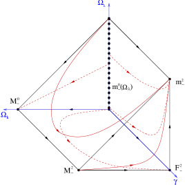
Figure 1: State space for the collapsing open FLRW models, $\epsilon=-1,~{}^{3}R\leq 0$. The bottom plane $\Omega_{\lambda}=0$ corresponds to general relativity. The top surface $\Omega_{k}+\Omega_{\lambda}=1$ corresponds to vacuum $\Omega_{\rho}=0$. The equilibrium points $M_{-}^{0},~{}M_{-}^{2},~{}F_{-}^{2},~{}m_{-}^{2},~{}m_{-}^{0}(\Omega_{\lambda})$ describe the Milne universe with $\gamma=0$ / stiff matter, the flat FLRW model with stiff matter, the non-general-relativistic BDL model with stiff matter and a line of non-general-relativistic models with constant energy density (including the flat FLRW model with $\gamma=0$). We are only drawing the trajectories in the invariant planes, from which the whole dynamics can be deduced. The structure of this part of the whole state space does not change with the parameter value $b$. The full state space can be obtained by matching this section to FIG. 2 - FIG. 9.

The bottom planes in Figures 1 - 9 correspond to GR, while top planes represent the vacuum boundaries.

Since the eigenvalues of the equilibrium points in general depend on the parameter $b$, the nature of these critical points varies with $b$. Furthermore, some of the critical points ($F_{+}^{b^{2}/3},~{}X_{+}^{2/3}$) will also move in state space as $b^{2}$ increases, since their coordinates are also functions of $b$. We also find critical points, which only appear for $b=0$ and then disappear, as we increase $b^{2}$.

For certain values of $b$, some of the eigenvalues pass through zero. At these values of $b$, the state space is “torn” in that it undergoes topological changes. In contrast to the model that Campos analysed, the appearance of such bifurcations in our model does not coincide with the appearance of lines of critical points. This a consequence of the fact, that in our inflationary model, the critical points are moving in state space. Bifurcations appear, when two of the equilibrium points merge, which occurs at $b^{2}=0,2,6$. These are the same parameter values as in GR Burd ; Halliwell . This was to be expected, since the only points moving in state space and causing these bifurcations, are the ones corresponding to the general relativistic models $F_{+}^{b^{2}/3},~{}X_{+}^{2/3}$. For this reason the occurrence of bifurcations is restricted to the GR - subspace. Therefore the dynamics of these bifurcations will only be discussed in section V.1.

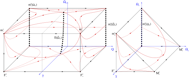
Figure 2: State space for the FLRW models with non-negative spatial curvature ${}^{3}R\geq 0,~{}\epsilon=\pm 1$ (on the left) and the expanding FLRW models with non-positive spatial curvature, ${}^{3}R\leq 0,~{}\epsilon=1$ (on the right) for $b=0$ (a bifurcation). In the left part of the figure, which describes the closed models, the plane $Q=0$ differentiates between the expanding sector $Q\geq 0,~{}\epsilon=1$ and the collapsing sector $Q\leq 0,~{}\epsilon=-1$. As in FIG. 1, the bottom plane corresponds to GR, whereas the top surfaces represent the vacuum solutions. We only give the trajectories on the invariant planes, from which the whole dynamics can be deduced. The critical points $F_{\epsilon}^{2},~{}m_{\epsilon}^{2},~{}m_{\epsilon}^{0}(\tilde{\Omega}_{\lambda}),~{}E(\tilde{\Omega}_{\lambda})$ correspond to the flat FLRW model with stiff matter, the non-general-relativistic BDL model with stiff matter, a line of non-general relativistic model with constant energy density (including the flat FLRW model with $\gamma=0$) and a line of static Einstein universes with $1/3\leq\gamma\leq 2/3$.

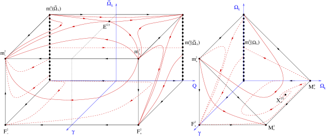
Figure 9: State space for the FLRW models with $b^{2}>6$. The model $F_{+}^{b^{2}/3}$ has moved out of state space, while $X_{+}^{2/3}$ is approaching the open vacuum boundary of the GR-subspace. See the captions of FIG. 1, FIG. 2 for more details.

Since the collapsing open sector remains unchanged with varying parameter value $b$, we do not include that sector in the different portraits of state space. The whole state space can be obtained by matching Fig. 1 to Fig. 2 - Fig. 9.

Table 3: Dynamical character of the critical points with non - positive spatial curvature.

Model	$b=0$	$0<b^{2}<2$	$b^{2}=2$	$2<b^{2}<\frac{8}{3}$	$b^{2}=\frac{8}{3}$	$\frac{8}{3}<b^{2}<6$	$b^{2}=6$	$b^{2}>6$
$\mbox{m}_{+}^{0}(\Omega_{\lambda})$	line of sinks	line of saddles	line of saddles	line of saddles	line of saddles	line of saddles	line of saddles	line of saddles
$\mbox{m}_{-}^{0}(\Omega_{\lambda})$	line of sources	line of sources	line of sources	line of sources	line of sources	line of sources	line of sources	line of sources
$\mbox{M}_{\epsilon}^{0}$	saddle	saddle	saddle	saddle	saddle	saddle	saddle	saddle
$\mbox{M}_{\epsilon}^{2}$	saddle	saddle	saddle	saddle	saddle	saddle	saddle	saddle
$\mbox{F}_{+}^{2}$	saddle	saddle	saddle	saddle	saddle	saddle	saddle	saddle
$\mbox{F}_{-}^{2}$	saddle	saddle	saddle	saddle	saddle	saddle	saddle	saddle
$\mbox{m}_{+}^{2}$	source	source	source	source	source	source	source	source
$\mbox{m}_{-}^{2}$	sink	sink	sink	sink	sink	sink	sink	sink
$\mbox{F}_{+}^{b^{2}/3}$	line of sinks	sink	saddle	saddle	saddle	saddle	saddle	-
$\mbox{X}_{+}^{2/3}(b)$	$-$	-	saddle a	sink	sink	spiral sink	spiral sink	spiral sink

V.1 The GR - subspace

As discussed above, the subset $\Omega_{\lambda},\tilde{\Omega}_{\lambda}=0$ is the invariant submanifold of the full state space corresponding to GR. In this section, we will discuss the stability of the general relativistic equilibrium points within the GR - subspace. In the next section, we will discuss the brane - world - modifications of these general relativistic results due to the additional degrees of freedom $\Omega_{\lambda},~{}\tilde{\Omega}_{\lambda}$, and also the additional non - general relativistic equilibrium points.

It is worth mentioning that although the GR - submanifold has been discussed in detail by Burd and Barrow Burd and Halliwell Halliwell , their analysis is somewhat incomplete, since the state space they considered was non - compact. The variables they chose to describe the inflationary dynamics of homogeneous isotropic models were $\phi^{\prime},\alpha^{\prime}$. Here $\alpha$ relates to the scale factor $a(\tau)$ by $a(\tau)=e^{\alpha(\tau)}$, and the potential has been absorbed into the time derivative by rescaling the time variable $t\rightarrow\tau$ by $\frac{d}{d\tau}=~{}^{\prime}~{}=V^{-1/2}\frac{d}{dt}$. We find that these coordinates relate to our expansion normalized variables via the following transformations:

$$(\alpha^{\prime})^{2}=\frac{2}{3}\frac{1}{(2-\gamma)(1-\Omega_{k})}\;,$$

$$(\phi^{\prime})^{2}=\frac{2\gamma}{2-\gamma}\;,$$

for $\gamma\neq 2,~{}\Omega_{k}\neq 1$. We can see that

$$\alpha^{\prime}\rightarrow\infty~{}\Leftrightarrow~{}\Omega_{k}\rightarrow 1~{}\Leftrightarrow~{}\Omega_{\rho}\rightarrow 0$$

and

$$\phi^{\prime}\rightarrow\infty~{}\Leftrightarrow~{}\gamma\rightarrow 2\;.$$

This means, that we have compactified the state space by mapping $\phi^{\prime}\in[0,\infty]\longrightarrow\gamma\in[0,2]$ and $\alpha^{\prime}\in[0,\infty]\longrightarrow\Omega_{k}\in[0,1]$. In this way we have extended the work that has been done on inflationary models with exponential potentials in the general relativistic context. We find that $X_{+}^{2/3},~{}F_{+}^{b^{2}/3}$ correspond to the critical points I, II in Burd . In addition, we obtain the new critical points $F_{\epsilon}^{2}$, $M_{\epsilon}^{0}$ and $M_{\epsilon}^{2}$ corresponding to a FLRW universe with stiff matter and a Milne universe with $\gamma=0$ or stiff matter $\gamma=2$ respectively.

Notice that we also find the new equilibrium point $F_{\epsilon}^{0}$. The reason is that we are using $\gamma$ to describe the dynamics of the scalar field $\phi$, which essentially is a function of $\dot{\phi}^{2}$ instead of $\dot{\phi}$. Therefore our $\dot{\gamma}$ - equation is homogeneous in $\dot{\phi}$, whereas the dynamical equation for $\dot{\phi}$ is inhomogeneous in $\dot{\phi}$.

It might seem surprising, that we find a critical point at $\dot{\phi}=0$, whereas there is no equilibrium point at $\dot{\phi}=0$ in Burd . The reason for this is, that we are describing different physical quantities; although the equation of state does not change as $\dot{\phi}\rightarrow 0~{}(\dot{\gamma}=0)$, $\dot{\phi}$ does change as $\dot{\phi}\rightarrow 0~{},(\ddot{\phi},\phi^{\prime\prime}\neq 0)$.

The collapsing FLRW model with stiff matter found in this analysis is of particular interest, since for all values of $b$, $F_{-}^{2}$ is the future attractor for all collapsing open and some of the closed models within the GR - subspace. $F_{-}^{0}$ is the past attractor for the whole collapsing open and parts of the closed sector for all $b$.

Notice that the dynamics of the collapsing open sector does not depend on the parameter value $b$. The dynamics of this sector is constrained by the fact, that for all models in this sector, the flat FLRW model with constant energy density is the past attractor, and the flat FLRW model with stiff matter is the future attractor (see FIG 1).

Having said that, we will now discuss the more complicated dynamics of the closed and the expanding open models for the different ranges of the parameter value $b$.

Table 4: Coordinates and eigenvalues of the critical points with non - negative spatial curvature. We have defined $\chi=\sqrt{\frac{8-3b^{2}}{2}},\phi=\sqrt{\tilde{\Omega}_{\lambda}^{2}+3\tilde{\Omega}_{\lambda}+1}$

Model	Coordinates	Eigenvalues
$\mbox{m}_{\epsilon}(\tilde{\Omega}_{\lambda}\neq 1)~{}for~{}b=0$	$(0,1,\tilde{\Omega}_{\lambda})$	$-2\epsilon(3,1,0)$
$\mbox{m}_{\epsilon}^{0}(\tilde{\Omega}_{\lambda}\neq 1)~{}for~{}b\neq 0$	$(0,1,\tilde{\Omega}_{\lambda})$	$(\infty,-2\epsilon,0)$
$\mbox{F}_{\epsilon}^{2}$	$(2,\epsilon,0)$	$(6\epsilon+\sqrt{6}b,4\epsilon,-6\epsilon)$
$\mbox{m}_{\epsilon}^{2}$	$(2,\epsilon,1)$	$2\epsilon(3,5,3)$
$\mbox{F}_{+}^{b^{2}/3}$	$(\frac{b^{2}}{3},1,0)$	$(\frac{b^{2}}{2}-3,b^{2}-2,-b^{2})$
$\mbox{X}_{+}^{2/3}(b)$	$(\frac{2}{3},-\frac{b}{\sqrt{2}},0)$	$(\frac{b}{\sqrt{2}}-\chi,\frac{b}{\sqrt{2}}+\chi,\sqrt{2}b)$
$\mbox{E}^{1/3}~{}$	$(\frac{1}{3},0,1)$	$(\sqrt{5},-\sqrt{5},0)$
$\mbox{E}(\tilde{\Omega}_{\lambda})~{}for~{}b=0$	$(\frac{2}{3(1+\tilde{\Omega}_{\lambda})},0,\tilde{\Omega}_{\lambda})$	$(\frac{2}{1+\tilde{\Omega}_{\lambda}}\phi,-\frac{2}{1+\tilde{\Omega}_{\lambda}}\phi,0)$

At $b=0$, we find a bifurcation of the state space, since for this value of $b$, the equilibrium points $E^{1/3}$ and $X_{+}^{2/3}(b)$, as well as $F_{+}^{0}$ and $F_{+}^{b^{2}/3}$ coincide. All expanding open models are attracted to $F_{+}^{0}$. All closed models will evolve into either $F_{-}^{2}$ or $F_{+}^{0}$, depending on the initial conditions. At $\gamma=2/3$, the Einstein universe appears as an unstable saddle point (see FIG 2).

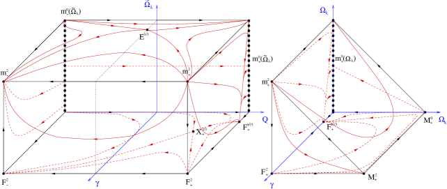
Figure 3: State space for the FLRW models with $0<b^{2}<2$. The line of Einstein universes in the closed sector of the state space has collapsed into the non-general-relativistic Einstein model $E^{1/3}$ and the general-relativistic model $X_{+}^{2/3}$, which is expanding and moving towards the expanding flat subspace $Q=1$, ($\epsilon=1$) as $b^{2}$ is increasing. The equilibrium point $F_{+}^{b^{2}/3}$ corresponds to a flat FLRW model with $\gamma=b^{2}/3$. See the captions of FIG. 1, FIG. 2 for more details.

As $b^{2}$ increases, the Einstein universe disappears. Instead, we find the saddle point $X_{+}^{2/3}(b)$, which moves in $Q$ - direction as $b^{2}$ is increases, remaining a saddle until it reaches the flat sector $Q=1$ at $b^{2}=2$. There it merges with expanding FLRW model $F_{+}^{b^{2}/3}$. For $0<b^{2}<2$, $F_{+}^{b^{2}/3}$ is a sink moving along the $\gamma$ - axis. All open and some of the closed models are attracted to this solution (see FIG 3).

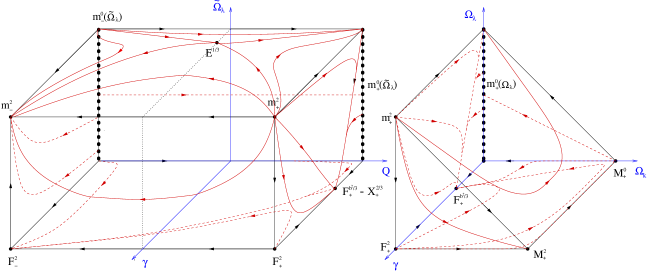
Figure 4: State space for the FLRW models with $b^{2}=2$ (a bifurcation). The equilibrium point $X_{+}^{2/3}$ has reached the flat subspace, where it merges with $F_{+}^{b^{2}/3}$. This causes the bifurcation; the nature of the two critical points will be swapped as they are moving on (see FIG. 5 - 9). All open and flat models are attracted to this point $X_{+}^{2/3}=F_{+}^{b^{2}/3}$, whereas all closed models are repelled. See the captions of FIG. 1, FIG. 2 for more details.

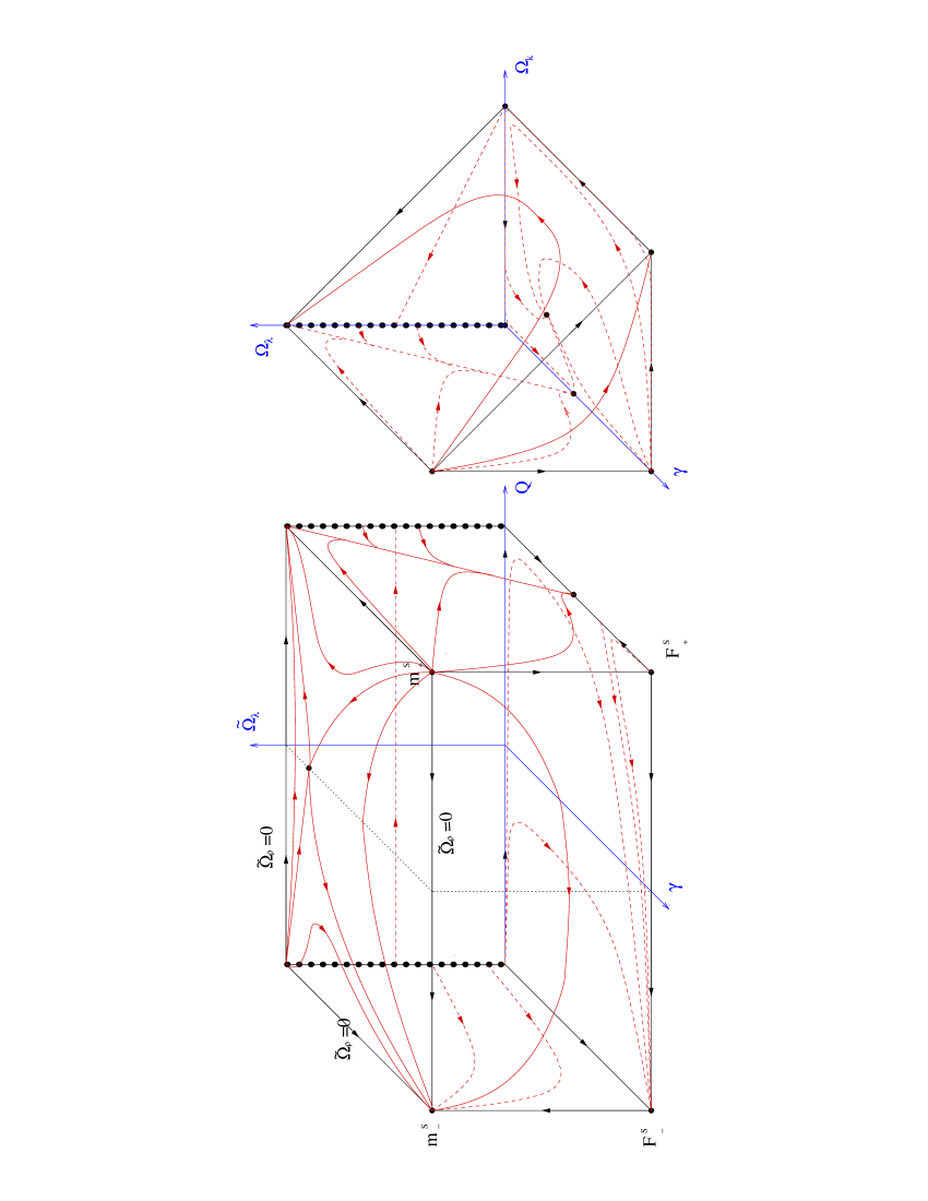
Figure 5: State space for the FLRW models with $2<b^{2}<8/3$. $X_{+}^{2/3}$ has entered the open sector and turned into a node sink. $F_{+}^{b^{2}/3}$ is now an unstable saddle for all models. See the captions of FIG. 1, FIG. 2 for more details.

At $b^{2}=2$, the models $X_{+}^{2/3}(b)$ and $F_{+}^{b^{2}/3}$ merge, which causes a bifurcation of the state space. The nature of the two merging critical points is significantly changed at this value of $b$. The flat solution $X_{+}^{2/3}(b=-\sqrt{2})=F_{+}^{2/3}$ is an attractor for all open or flat models, but a repeller for all closed models (see FIG 4). This behaviour has been observed by Burd . At this value of $b^{2}$, the two merging critical points swap their nature: for all $b^{2}\geq 2$, $X_{+}^{2/3}(b)$ will be a sink, while $F_{+}^{b^{2}/3}$ will be a saddle (see FIGS 5 - 9).

As $b$ is further increased ($2<b^{2}<6$), $F_{+}^{b^{2}/3}$ moves further along the $\gamma$ - axis. It is now a saddle for all models. All flat models are attracted, whereas all open or closed models are repelled. $X_{+}^{2/3}(b)$ has now entered the open sector and moves further to the $\Omega_{k}=1$ boundary. $X_{+}^{2/3}(b)$ is a node sink for all $2<b^{2}<8/3$ and a spiral sink for $8/3<b^{2}<\infty$. For all $b^{2}\geq 2,~{}F_{-}^{2}$ is the future attractor for all closed models and $X_{+}^{2/3}(b)$ the future attractor for all expanding open models (see FIGS 5 - 7).

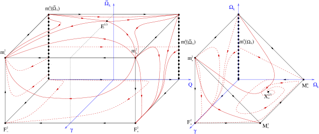
Figure 8: State space for the FLRW models with $b^{2}=6$ (a bifurcation). The equilibrium point $F_{+}^{b^{2}/3}$ has merged with the equilibrium point $F_{+}^{2}$, which causes the bifurcation. The topology of the state space is changing at this value of $b$, since the point $F_{+}^{2}$ is turning from an attractor in $\gamma$-direction into a repeller in that direction (compare to FIG. 7, FIG. 9). See the caption of FIG. 1, FIG. 2 for more details.

At $b^{2}=6$, we find another bifurcation of the state space. The two points $F_{+}^{b^{2}/3}$ and $F_{+}^{2}$ merge. This turns $F_{+}^{2}$ from a source into a saddle (see FIG. 8). For $b^{2}\geq 6$, all open or closed models are still repelled from $F_{+}^{2}$, but all flat models are now attracted. In the limit $b^{2}\rightarrow\infty$, the future attractor for the open sector, $X_{+}^{2/3}(b)$ approaches the vacuum solution $\Omega_{\rho}\rightarrow 0$ with $\gamma=2/3$ (see FIG 9).

Table 5: Eigenvalues and eigenvectors of the critical points with non-negative spatial curvature ${}^{3}R\geq 0$. We have defined $\chi=\sqrt{\frac{8-3b^{2}}{2}}$, $\phi=\sqrt{\tilde{\Omega}_{\lambda}^{2}+3\tilde{\Omega}_{\lambda}+1}$. Notice that the first eigenvector of second row is $(-6\epsilon-\sqrt{3}b\sqrt{\frac{1-\tilde{\Omega}_{\lambda}}{\gamma}},0,3\tilde{\Omega}_{\lambda}(\tilde{\Omega}_{\lambda}-1))\longrightarrow(1,0,0)$ as $\gamma\rightarrow 0$ for $\tilde{\Omega}_{\lambda}\neq 1$.

Model	Eigenvalues	Eigenvectors
$\mbox{m}_{\epsilon}^{0}(\tilde{\Omega}_{\lambda}\neq 1)~{}for~{}b=0$	$\epsilon(-6,-2,0)$	$(2,0,\tilde{\Omega}_{\lambda}(1-\tilde{\Omega}_{\lambda})),(0,1,0),(0,0,1)$
$\mbox{m}_{\epsilon}^{0}(\tilde{\Omega}_{\lambda}\neq 1)~{}for~{}b\neq 0$	$(\infty,-2\epsilon,0)$	$(1,0,0),(0,1,0),(0,0,1)$
$\mbox{F}_{\epsilon}^{2}$	$(6\epsilon+\sqrt{6}b,4\epsilon,-6\epsilon)$	$(1,0,0),(0,1,0),(0,0,1)$
$\mbox{m}_{\epsilon}^{2}$	$2\epsilon(3,5,3)$	$(1,0,0),(0,1,0),(0,0,1)$
$\mbox{F}_{+}^{b^{2}/3}$	$(\frac{b^{2}}{2}-3,b^{2}-2,-b^{2})$	$(1,0,0),(b^{2}(\frac{b^{2}}{3}-2),\frac{b^{2}}{2}+1,0),(b^{2}(1-\frac{b^{2}}{6}),0,3(\frac{b^{2}}{2}-1))$
$\mbox{X}_{+}^{2/3}(b)$	$(\frac{b}{\sqrt{2}}-\chi,\frac{b}{\sqrt{2}}+\chi,\sqrt{2}b)$	$(\frac{8}{3},\frac{b}{\sqrt{2}}+\chi,0),(\frac{8}{3},\frac{b}{\sqrt{2}}-\chi,0),(2,\frac{3}{2\sqrt{2}}b(1-\frac{b^{2}}{2}),3(1-\frac{b^{2}}{2}))$
$\mbox{E}^{1/3}~{}$	$(\sqrt{5},-\sqrt{5},0)$	$(\sqrt{5},-3,0),(\sqrt{5},3,0),-$
$\mbox{E}(\tilde{\Omega}_{\lambda})~{}for~{}b=0$	$(\frac{2}{1+\tilde{\Omega}_{\lambda}}\phi,-\frac{2}{1+\tilde{\Omega}_{\lambda}}\phi,0)$	$(-\frac{4+6\tilde{\Omega}_{\lambda}}{3(1+\tilde{\Omega}_{\lambda})},\phi,\tilde{\Omega}_{\lambda}(\tilde{\Omega}_{\lambda}-1)),(\frac{4+6\tilde{\Omega}_{\lambda}}{3(1+\tilde{\Omega}_{\lambda})},\phi,-\tilde{\Omega}_{\lambda}(\tilde{\Omega}_{\lambda}-1)),(1,0,-\frac{3}{2}(1+\tilde{\Omega}_{\lambda})^{2})$

V.2 Higher dimensional effects

The question we will now discuss is how the behaviour of the dynamical system describing GR is changed within the brane - world context. In particular, do the additional degree of freedom $\Omega_{\lambda},~{}\tilde{\Omega}_{\lambda}$ change the stability of the general relativistic models, and are there new non - general relativistic stable equilibrium points?

We will first answer the second question. In addition to the general relativistic points, we have found the non - general - relativistic equilibrium points $m_{\epsilon}^{2}$ and the lines $m_{\epsilon}^{0}(\Omega_{\lambda})$. We can solve the Friedmann equation at these points to determine their behaviour in detail. At $m_{\epsilon}^{0}$, the energy density is constant $\rho(t)=\rho_{0}$, and we can easily integrate the Friedmann equation to find

$$a(t)\sim e^{\epsilon\sqrt{\tilde{\Lambda}/3}~{}t}\;,$$ (31)

where $\tilde{\Lambda}=\kappa^{2}\rho_{0}(1+{\textstyle{\frac{\rho_{0}}{2\lambda}}})$ behaves like a modified cosmological constant.

For $m_{+}^{2}$, the scale factor is given by

$$a(t)=(t-t_{BB})^{1/6}(t+t_{BB})^{1/6}\;.$$ (32)

where $t_{BB}=1/\sqrt{6\kappa^{2}\lambda}$ is the Big Bang time. As explained in detail in Campos , this model corresponds to the Binétruy - Deffayet - Langlois (BDL) solution Binetruy with scale factor $a(t)=(t-t_{BB})^{1/6}$. The solution for $m_{-}^{2}$ is given by time reversal and $t_{BB}$ should now be identified as the Big Crunch time.

At $b=0$, we also observe, that the general - relativistic Einstein universe has non - general - relativistic analogues. We find a whole line of Einstein universe - like static equilibrium points $E(\tilde{\Omega}_{\lambda})$ extending in the $\tilde{\Omega}_{\lambda}$ direction. For $b^{2}>0$, the line collapses to the non - general - relativistic Einstein saddle $E^{1/3}$ in the $\tilde{\Omega}_{\lambda}=1$ subset, and the general relativistic model $X_{+}^{2/3}(b)$.

We now study the dynamical character of these non - general - relativistic equilibrium points. We find that in the full state space, $m_{-}^{2}$ instead of $F_{-}^{2}$ is the future attractor for all collapsing open models and some of the closed models. This means, that within the brane - world context, FLRW with stiff matter changes from a stable solution into a unstable saddle. $F_{-}^{0}$ remains a past attractor for the collapsing open and parts of the closed sector, but now there is a whole line $m_{-}^{0}(\Omega_{\lambda})$ of sources extending in $\tilde{\Omega}_{\lambda}$ direction. The same applies to the corresponding expanding models: the sink/saddle $F_{+}^{0}$ is a one - element subset of the line of sinks/saddles $m_{+}^{0}(\Omega_{\lambda})$. This means, that for $b=0$, the future attractor of the expanding open and some of the closed models is not necessarily $F_{+}^{0}$, but instead any of the points $m_{+}^{0}(\Omega_{\lambda})$ depending on the initial conditions. For $b^{2}>0$, $m_{+}^{0}(\Omega_{\lambda})$ including $F_{+}^{0}$ turns into a line of saddles.

For $b>0$ the models $m_{+}^{0}(\Omega_{\lambda})$ represent high energy inflationary models with exponential potentials (which are too steep to inflate in GR) Copeland . The fact that they are all unstable (saddle points) reflects the fact that steep inflation ends naturally, since as the energy drops below the brane tension the condition for inflation no longer holds.

Finally let us consider whether the stability of the most interesting equilibrium points $F_{+}^{b^{2}/3}$ and $X_{+}^{2/3}$ is changed by the higher - dimensional degrees of freedom. From Tables V, VI, we can see that the third eigenvalues (corresponding to eigenvectors pointing out of the GR - plane) are negative for all $b\neq 0$. That means, if $F_{+}^{b^{2}/3}$, $X_{+}^{2/3}$ was a sink in GR, it will remain a sink in the brane - world scenario.

Table 6: Dynamical character of the critical points with non - negative spatial curvature.

Model	$b=0$	$0<b^{2}<2$	$b^{2}=2$	$2<b^{2}<6$	$b^{2}=6$	$b^{2}>6$
$\mbox{m}_{+}^{0}(\tilde{\Omega}_{\lambda})$	line of sinks	line of saddles	line of saddles	line of saddles	line of saddles	line of saddles
$\mbox{m}_{-}^{0}(\tilde{\Omega}_{\lambda})$	line of sources	line of sources	line of sources	line of sources	line of sources	line of sources
$\mbox{F}_{+}^{2}$	saddle	saddle	saddle	saddle	saddle	saddle
$\mbox{F}_{-}^{2}$	saddle	saddle	saddle	saddle	saddle	saddle
$\mbox{m}_{+}^{2}$	source	source	source	source	source	source
$\mbox{m}_{-}^{2}$	sink	sink	sink	sink	sink	sink
$\mbox{F}_{+}^{b^{2}/3}$	line of sinks	sink	saddle	saddle	saddle	-
$\mbox{X}_{+}^{2/3}(b)$	line of saddles	saddle	saddle a	-	-	-
$\mbox{E}^{1/3}$	saddle	saddle	saddle	saddle	saddle	saddle
$\mbox{E}(\tilde{\Omega}_{\lambda})~{}for~{}b=0$	line of saddles	-	-	-	-	-

VI Discussion and Conclusion

In this paper we extend recent work by Campos and Sopuerta Campos to the case where the matter is described by a dynamical scalar field $\phi$ with an exponential potential. By using expansion normalised variables which compactifies the state space we built on earlier results due to Burd and Barrow Burd and Halliwell Halliwell for the case of GR and explored the effects induced by higher dimensions in the brane - world scenario.

As in Campos we obtain the equilibrium point corresponding to the BDL model ($\mbox{m}_{\pm}$) Binetruy which dominates the dynamics at high energies (near the Big Bang and Big Crunch), where the extra - dimension effects become dominant supporting the claim that this solution is a generic feature of the state space of more general cosmological models in the brane - world scenario.

We emphasise again that here, unlike in the analysis by Campos and Sopuerta Campos , $\gamma$ is a dynamical variable. Fixing $\gamma$ to be a constant corresponds to looking at the $\gamma=const.$ slices of the full state space. This obviously only makes sense for the invariant sets $\gamma=0$ and $\gamma=2$. The important point is, that even if we want to analyse the dynamical character of the de Sitter and Milne models in the $\gamma=0$ - plane, we have to bear in mind the dynamical character of $\gamma$. Unlike in Campos , we have to study perturbations away from the plane. This makes these models much more interesting in the presence of an exponential potential, since the dynamics are not reduced to the plane $\gamma=0$. In fact, unless $b=0$, we find that the plane $\gamma=0$ is unstable. Small perturbations out of that plane will in general be enhanced, i.e. even for initial conditions with negligible $\gamma$, the system will in general evolve towards $\gamma=2/3$ or $\gamma=2$. Notice that orbits confined to the $\gamma=0$ plane evolve towards the expanding de Sitter models $m^{0}_{+}(\Omega_{\lambda})$ or the contracting Milne universe $M^{0}_{-}$ for all values of $b$.

Finally we note that we did not find any new bifurcations in this simple brane - world scenario because we consider only the case ${\cal U}=0$. In the next paper in this series paper2 we will analyse both the effects of the non - local energy density ${\cal U}$ on the FLRW brane - world dynamics and look at homogeneous and anisotropic models with an exponential potential.

Acknowledgments: We would like to thank Roy Maartens and Varun Sahni for very useful discussions during the Cape Town Cosmology Meeting in July 2001. We also thank Toni Campos and Carlos Souperta for comments and suggestions for future work. This work has been funded by the National Research Foundation (SA) and a UCT international postgraduate scholarship.

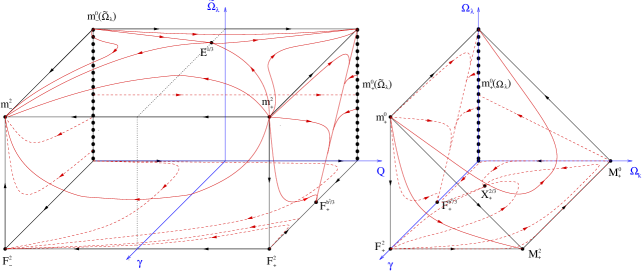
Figure 6: State space for the FLRW models with $b^{2}=8/3$. The node sink $X_{+}^{2/3}$ is turning into a spiral sink; the structure of the state space has not changed. See the captions of FIG. 1, FIG. 2 for more details.

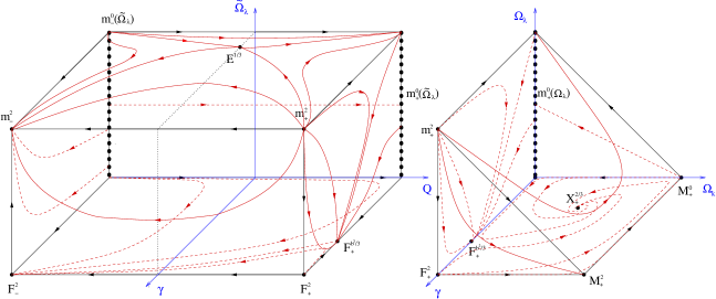
Figure 7: State space for the FLRW models with $8/3<b^{2}<6$. $X_{+}^{2/3}$ is now a spiral sink; the structure of the state space is essentially the same as for $2<b^{2}\leq 8/3$. See the captions of FIG. 1, FIG. 2 for more details.

References

- (1) P. Hoava and E. Witten, Nucl. Phys. B460, 506 (1996).
- (2) P. Hoava and E. Witten, Nucl. Phys. B475, 94 (1996).
- (3) L. Randall and R. Sundrum, Phys. Rev. Lett. 83, 4690 (1999).
- (4) V. A. Rubakov and M. E. Shaposhnikov, Phys. Lett. B 125, 136 (1983); M. Visser, ibid. 159, 22 (1985); E. J. Squires, ibid. 167, 286 (1986); M. Gell - Mann and B. Zwiebach, Nucl. Phys. B260, 569 (1985); H. Nicolai and C. Wetterich, Phys. Lett. B 150, 347 (1985); M. Gogberashvili, Mod. Phys. Lett. A 14, 2025 (1999). K. Akama, in Lectures in Physics, Vol. 176, edited by K. Kikkawa, N. Nakanishi, and H. Nariai (Springer Verlag, New York, 1982).
- (5) M. Goliath and G. F. R. Ellis, Phys. Rev. D 60, 023502 (1999).
- (6) J. Wainwright and G. F. R. Ellis, Dynamical systems in cosmology (Cambridge University Press, Cambridge, 1997).
- (7) A. Campos and C. F. Sopuerta, Phys. Rev. D 63, 104012 (2001).
- (8) P. Bintruy, C. Deffayet, and D. Langlois, Nucl. Phys. B565, 269 (2000).
- (9) R. Maartens. V. Sahni and T. D. Saini, Phys. Rev. D 63, 063509 (2001).
- (10) A. D. Burd and John D. Barrow, Nucl. Phys. B308, 929 (1988).
- (11) J. J. Halliwell, Phys. Lett. B 185, no.3,4 (1987).
- (12) R. J. van den Hoogen, A. A. Coley and D. Wands, Class. Quantum Grav. 16, 1843 (1999)
- (13) E. J. Copeland, A. R. Liddle and D. Wands, Phys. Rev. D 57, 4686 (1998).
- (14) E. J. Copeland, A. R. Liddle and J. E. Lidsey, astro-ph/000642.
- (15) T. Shiromizu, K. Maeda, and M. Sasaki, Phys. Rev. D 62, 024012 (2000).
- (16) M. Sasaki, T. Shiromizu, and K. Maeda, Phys. Rev. D 62, 024008 (2000).
- (17) R. Maartens, Phys. Rev. D 62, 084023 (2000).
- (18) M. Bruni, G. F. R. Ellis and P. K. S. Dunsby Class. Quant. Gravity 9, 921 (1991).
- (19) M. S. Madsen, Class. Quantum Grav., 5, 627 (1988).
- (20) N. Goheer and P. K. S. Dunsby, In Preparation (2002).