Supergravity Inflation on the Brane

Abstract

We study $N=1$ Supergravity inflation in the context of the braneworld scenario. Particular attention is paid to the problem of the onset of inflation at sub-Planckian field values and the ensued inflationary observables. We find that the so-called $\eta$-problem encountered in supergravity inspired inflationary models can be solved in the context of the braneworld scenario, for some range of the parameters involved. Furthermore, we obtain an upper bound on the scale of the fifth dimension, $M_{5}\mathrel{\hbox to0.0pt{\lower 4.0pt\hbox{\hskip 1.0pt$\sim$}\hss}\raise 1.0pt\hbox{$<$}}10^{-3}M_{P}$, in case the inflationary potential is quadratic in the inflaton field, $\phi$. If the inflationary potential is cubic in $\phi$, consistency with observational data requires that $M_{5}\simeq 9.2\times 10^{-4}M_{P}$.

I Introduction

In supersymmetric theories with a single supersymmetry generator ($N=1$), complex scalar fields are the lowest components, $\phi^{a}$, of chiral superfields $\Phi^{a}$. Masses for fields will be generated by spontaneous symmetry breaking so that the only fundamental mass scale is the reduced Planck mass, $M=M_{P}/\sqrt{8\pi}$. The $N=1$ supergravity theory describing the interaction of the chiral superfields, the scalar potential is given by

$$V={\rm e}^{K/M^{2}}\left[F^{A\dagger}(K_{A}^{B})^{-1}F_{B}-3{|W|^{2}\over M^{2}}\right]+{\rm D-terms}~{}~{},$$ (1)

where

$$F_{A}\equiv{\partial W\over\partial\Phi^{A}}+\left({\partial K\over\partial\Phi^{A}}\right){W\over M^{2}},~{}~{}K_{A}^{B}\equiv{\partial^{2}K\over\partial\Phi^{A}\partial\Phi_{B}^{\dagger}}~{}.$$ (2)

The Kähler function, $K$, sets the form of the kinetic energy terms of the theory while the superpotential, $W$, determines the non-gauge interactions. For canonical kinetic energy terms, $K=\sum_{A}\phi_{A}^{\dagger}\phi^{A}$, the potential takes the relatively simple form

$$V=\exp\left(\sum_{A}{\phi_{A}^{\dagger}\phi^{A}\over M^{2}}\right)\left[\sum_{B}\left|{\partial W\over\partial\phi_{B}}\right|^{2}-3{\left|W\right|^{2}\over M^{2}}\right]~{}.$$ (3)

Expanding the (slowly varying) inflaton potential about the value of the inflaton field at which the quantum fluctuations of interest are produced giving rise to structure formation, $\tilde{\phi}$, by writing $\varphi={\tilde{\phi}}+\phi$, we obtain a polynomial potential in $\phi$

$$V=\Delta^{4}\left[1+c_{1}{\phi\over M}+c_{2}\left(\phi\over M\right)^{2}+\cdots\right]~{}~{},$$ (4)

where we have factored out the mass parameter $\Delta$, which sets the scale of the inflationary phase and can be directly related with the amplitude of energy density perturbations. In this work, we shall consider a class of models in which the evolution of the inflaton dynamics is controlled by a single power at the point where the observed density fluctuations are produced; in this case, the potential assumes the following form

$$V\simeq\Delta^{4}\left[1+c_{n}\left(\phi\over M\right)^{n}\right]~{}~{}.$$ (5)

The case where the second term is dominant and $n=2$, a situation typical of chaotic inflationary models, has already been analysed in Refs. Maartens ; Bento1 , where it is shown that specific features of the braneworld scenario allow for current observational constraints to be successfully accounted for with a single scale at the superpotential level; hence, difficulties with higher order non-renormalizable terms can be quite naturally avoided since it is possible to achieve successful inflation with sub-Planckian field values.

In this work, we consider the case where the first term is dominant and $n=2$ or $n=3$; regarding the former case, it is well known that a generic supergravity theory gives contributions of order $\pm H^{2}$ Bertolami to the inflaton mass squared whereas inflation requires $|m^{2}|\ll H^{2}$, this is the so-called $\eta$ problem. We will show that, in the braneworld scenario, this problem can be avoided, provided the $D=5$ Planck mass satisfies the condition $M_{5}\mathrel{\hbox to0.0pt{\lower 4.0pt\hbox{\hskip 1.0pt$\sim$}\hss}\raise 1.0pt\hbox{$<$}}10^{16}~{}\mbox{GeV}$. This kind of analysis has recently been done for a particular supergravity F-term hybrid inflation model JohnM , namely the one of Ref. Dvali . It is relevant to point out that hybrid inflationary models Linde ; Cope allow, as a result of the dynamics of two or more scalar fields, for successful realizations of the old inflationary type models, but have, in some instances, difficulties in what concerns initial conditions. However, these problems are shown to be naturally solved in braneworld scenarios in the case where the potential is dominated by the mass term Mendes .

We shall also consider the case where the quadratic term gets cancelled and, therefore, the inflationary potential is cubic in $\phi$, as is the case of the supergravity natural inflation model of Ref. Adams . We show that this model works in the braneworld scenario provided $M_{5}\simeq 1.1\times 10^{16}~{}\mbox{GeV}$.

II Requirements on the inflationary potential

We shall consider the five-dimensional brane scenario, where one assumes that Einstein equations with a negative cosmological constant hold (an anti-De-Sitter space is required) in $D$-dimensions and that matter fields are confined to the $3$-brane; then, the $4$-dimensional Einstein equation is given by Shiromizu :

$$G_{\mu\nu}=-\Lambda g_{\mu\nu}+{8\pi\over M_{P}^{2}}T_{\mu\nu}+\left({8\pi\over M_{5}^{3}}\right)^{2}S_{\mu\nu}-E_{\mu\nu}~{},$$ (6)

where $T_{\mu\nu}$ is the energy-momentum on the brane, $S_{\mu\nu}$ is a tensor that contains contributions that are quadratic in $T_{\mu\nu}$ and $E_{\mu\nu}$ corresponds to the projection of the 5-dimensional Weyl tensor on the 3-brane (physically, for a perfect fluid, it is associated to non-local contributions to the pressure and energy flux). In a cosmological framework, where the 3-brane resembles our universe and the metric projected onto the brane is an homogeneous and isotropic flat Friedmann-Robertson-Walker (FRW) metric, the Friedmann equation becomes Shiromizu ; Binetruy :

$$H^{2}={\Lambda\over 3}+\left({8\pi\over 3M_{P}^{2}}\right)\rho+\left({4\pi\over 3M_{5}^{3}}\right)^{2}\rho^{2}+{\epsilon\over a^{4}},$$ (7)

where $\epsilon$ is an integration constant. The four and five-dimensional cosmological constants are related by

$$\Lambda={4\pi\over M_{5}^{3}}\left(\Lambda_{5}+{4\pi\over 3M_{5}^{3}}~{}\lambda^{2}\right)~{}~{},$$ (8)

where $\lambda$ is the 3-brane tension, and the four and five-dimensional Planck scales through

$$M_{P}=\sqrt{{3\over 4\pi}}{M_{5}^{3}\over\sqrt{\lambda}}~{}~{}.$$ (9)

Assuming that, as required by observations, the cosmological constant is negligible in the early universe and since the last term in Eq. (7) rapidly becomes unimportant after inflation sets in, the Friedmann equation becomes

$$H^{2} = {8\pi\over 3M_{P}^{2}}\rho\left[1+{\rho\over 2\lambda}\right]$$ (10)

$$= \left(4\pi\over 3M_{5}^{3}\right)^{2}\rho^{2}\left(1+{\rho_{c}\over\rho}\right)~{},$$ (11)

with

$$\rho_{c}={3\over 2\pi}{M_{5}^{6}\over M_{P}^{2}}~{}~{}.$$ (12)

Hence, the new term in $\rho^{2}$ is dominant at high energies, compared to $\lambda^{1/4}$, i.e. $\rho>\rho_{c}$, but quickly decays at lower energies, and the usual four-dimensional FRW cosmology is recovered.

Consistently, we shall assume that the scalar field is confined to the brane, so that its field equation has the standard form

$$\ddot{\phi}+3H\dot{\phi}=-{dV\over d\phi}~{}.$$ (13)

Consistency between the slow-roll approximation and the full evolution equations requires that there are constraints on the slope and curvature of the potential. One can define two slow-roll parameters Maartens

$$\epsilon \equiv {M_{P}^{2}\over 16\pi}\left({V^{\prime}\over V}\right)^{2}{1+{V/\lambda}\over(2+{V/\lambda})^{2}}~{}~{},$$ (14)

$$\eta \equiv {M_{P}^{2}\over 8\pi}\left({V^{\prime\prime}\over V}\right){1\over 1+{V/2\lambda}}~{}~{}.$$ (15)

Notice that both parameters are suppressed by an extra factor $\lambda/V$ at high energies and that, at low energies, $V\ll\lambda$, they reduce to the standard form. The value of $\phi$ at the end of inflation can be obtained from the condition

$${\rm max}\{\epsilon(\phi_{F}),|\eta(\phi_{F})|\}=1~{}~{}.$$ (16)

The number of e-folds during inflation is given by $N=\int_{t_{\rm i}}^{t_{\rm f}}Hdt$, which becomes Maartens

$$N\simeq-{8\pi\over M_{P}^{2}}\int_{\phi_{\rm i}}^{\phi_{\rm f}}{V\over V^{\prime}}\left[1+{V\over 2\lambda}\right]d\phi~{}~{},$$ (17)

in the slow-roll approximation. We see that, as a result of the modification in the Friedmann equation, the expansion rate is increased, at high energies, by a factor $V/2\lambda$.

The amplitude of scalar perturbations is given by Maartens

$$A_{s}^{2}\simeq\left.\left({512\pi\over 75M_{P}^{6}}\right){V^{3}\over V^{\prime 2}}\left[1+{V\over 2\lambda}\right]^{3}\right|_{k=aH}~{}~{},$$ (18)

where the right-hand side should be evaluated as the comoving scale equals the Hubble radius during inflation, $k=aH$. Thus the amplitude of scalar perturbations is increased relative to the standard result at a fixed value of $\phi$ for a given potential.

The scale-dependence of the perturbations is described by the spectral tilt Maartens

$$n_{s}-1\equiv{d\ln A_{s}^{2}\over d\ln k}\simeq-6\epsilon+2\eta~{}~{},$$ (19)

where the slow-roll parameters are given in Eqs. (14) and (15). Notice that, as $V/\lambda\rightarrow\infty$, the spectral index of scalar perturbations is driven towards the Harrison-Zel’dovich spectrum, $n_{s}\rightarrow 1$.

Finally, the ratio between the amplitude of tensor and scalar perturbations is given by Langlois

$$\left({A_{t}\over A_{s}}\right)^{2}\simeq{3M_{P}^{2}\over 16\pi}\left({V^{\prime}\over V}\right)^{2}{2\lambda\over V}~{}~{}.$$ (20)

In what follows we shall use the inflationary observables defined to study two generic supergravity inflationary models of the type described by Eq. (5). We should stress that we shall be interested in achieving a sucessful inflationary scenario with sub-Planckian field values so as to avoid the abovementioned problems with higher order non-renormalizable terms.

III Quadratic potential

We first consider the case where the potential is quadratic in $\phi$ and we rewrite it as

$$V=V_{0}+{1\over 2}m^{2}\phi^{2}~{}~{},$$ (21)

and assume that the first term is dominant.

In supergravity, effective mass squared contributions of fields are given by Cope

$${1\over 2}m^{2}=8\pi{V_{0}\over M_{P}^{2}}\approx 3H^{2}$$ (22)

since the horizon of the inflationary De Sitter phase has a Hawking temperature given by $T_{H}=H/2\pi$ Bertolami .

Contributions like the ones of Eq. (22) lead to $\eta\equiv M_{P}^{2}V^{\prime\prime}/8\pi V\simeq 2$ ; however, the onset of inflation requires $\eta\ll 1$. Within the braneworld scenario, however, $\eta$ is modified, at high energies, by a factor $\lambda/V$ (see Eq. (15)). Hence, if the quantity, $\alpha\equiv V_{0}/\lambda$, is sufficiently large, this problem is automatically solved by the brane corrections, as in this case, $\eta\simeq 4/\alpha$ for large $\alpha$.

We shall now see that a constraint on $M_{5}$ can be obtained from the requirement that the magnitude of the energy density perturbations ensuing from our inflationary setup explains the anisotropies in the CMB radiation observed by COBE.

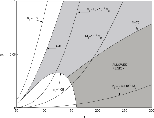
Figure 1: Contours of the inflationary observables $n_{s}$ and $r$ in the $\alpha,\beta$ plane. The requirement that the observational bounds on these quantities (cf. Eq.(27)) be respected, leads to the shaded regions; after the condition that there is sufficient inflation is applied, $N\geq 70$, only the dark grey region remains allowed. We also show contours corresponding to different values of $M_{5}$.

The number of $e$-foldings, $N$, in terms of $\alpha$ is given by

$$N=\alpha\left[{1\over 4}\log\left({\phi_{I}\over\phi_{F}}\right)+{2\pi\over M_{P}^{2}}(\phi_{I}^{2}-\phi_{F}^{2})+{16\pi^{2}\over M_{P}^{4}}(\phi_{I}^{4}-\phi_{F}^{4})\right]~{}.$$ (23)

Using the high energy approximation and $V\simeq V_{0}$ in Eq. (18), we obtain for $A_{s}^{2}$

$$A_{s}^{2}\simeq{64\pi\over 75M_{P}^{6}}{V_{0}^{6}\over\lambda^{3}m^{4}\phi_{\star}}~{}~{},$$ (24)

where $\phi_{\star}$ is the value of $\phi$ when scales corresponding to large-angle CMB anisotropies, as observed by COBE, left the Hubble radius during inflation. For $N_{\star}\approx 55$, $\phi_{I}=\phi_{\star}$ and $\phi_{F}=\beta M$ in Eq. (23), we get

$$\phi_{\star}\simeq 0.2\beta\exp\left(220\over\alpha\right)M_{P}~{}~{},$$ (25)

as, for sub-Planckian field values, the logarithmic term in Eq. (23) dominates. We prefer to leave $\phi_{F}$ as a free parameter since in hybrid models, which are of particular interest because they can give rise to quadratic potentials of the type we are studying once some other field is held at the origin by its interaction with $\phi$, inflation may end due to instabilities triggered by the dynamics of the other field. It then follows that the amount of inflation critically depends on the value of the inflaton field, $\phi_{F}$, and hence on $\beta$, at the time the instabilities arise. Notice that these instabilities are quite necessary in order to end inflation as $\epsilon=64\pi\phi^{2}/\alpha M_{P}^{2}<<1$ for $\alpha>>1$ and sub-Planckian field values. Moreover, it is clear that the condition $\epsilon\simeq 1$ cannot be met subsequently as the $\phi$ field is decreasing.

We also mention that the problem of initial conditions for hybrid models, discussed in Ref. Mendes , can also be solved in this model due to the brane corrections.

Inserting Eq. (25) into Eq. (24) and using the fact that the observed value from COBE is $A_{s}=2\times 10^{-5}$, we obtain for $M_{5}$:

$$M_{5}^{3}\simeq{8\pi\over\alpha^{2}}\times 10^{-5}\beta\exp(220/\alpha)~{}M_{P}^{3}~{}~{}.$$ (26)

Therefore, $M_{5}$ depends on the importance of the brane corrections via the $\alpha$ parameter and the value of the field at the end of inflation through $\beta$. In Figure 1, we show contours of the inflationary observables $n_{s}$ and $r\equiv 4\pi\left({A_{t}\over A_{s}}\right)^{2}$, as given by Eqs. (19) and (20), in terms of parameters $\alpha$ and $\beta$. The shaded regions in Figure 1 are obtained by requiring that the bounds resulting from latest CMB data from BOOMERANG Boom , and MAXIMA Maxima and DASI DASI

$$0.8<n_{s}<1.05~{}~{}~{},\qquad r<0.3~{}~{},$$ (27)

are satisfied. Also shown is the contour corresponding to $N=70$ (we have chosen the initial value of the inflaton field to be sub-Planckian, $\phi_{I}=0.2~{}M_{P}$) and, after applying the condition that there is sufficient inflation, $N\geq 70$, only the darker region remains allowed. This analysis clearly leads to a constraint on parameter $\alpha$, $\alpha\mathrel{\hbox to0.0pt{\lower 4.0pt\hbox{\hskip 1.0pt$\sim$}\hss}\raise 1.0pt\hbox{$>$}}140$. Finally, also in Figure 1, we have superposed contours of the scale $M_{5}$, from which we can derive an upper bound on this quantity

$$M_{5}\mathrel{\hbox to0.0pt{\lower 4.0pt\hbox{\hskip 1.0pt$\sim$}\hss}\raise 1.0pt\hbox{$<$}}10^{-3}M_{P}~{}~{}.$$ (28)

Finally, we mention that $\Delta$ (or instead $V_{0}$) in Eq. (5) can be estimated from the bound on the reheating temperature so as to avoid the gravitino problem (see Ref. Bento2 and references therein)

$$T_{RH} \mathrel{\hbox to0.0pt{\lower 4.0pt\hbox{\hskip 1.0pt$\sim$}\hss}\raise 1.0pt\hbox{$<$}} 2\times 10^{9}~{}\mbox{GeV}~{}~{},~{}~{}6\times 10^{9}~{}\mbox{GeV}~{},$$

$$\mbox{for}~{}~{}~{}~{}m_{3/2} = 1~{}\mbox{TeV}~{}~{},~{}~{}10~{}\mbox{TeV}~{}~{},$$ (29)

leading to $\Delta\mathrel{\hbox to0.0pt{\lower 4.0pt\hbox{\hskip 1.0pt$\sim$}\hss}\raise 1.0pt\hbox{$<$}}6.71\times 10^{-4}~{}M_{P}$, as the reheating temperature is given by Ross

$$T_{RH}\simeq 5.5\times 10^{-1}{\Delta^{3}\over M_{P}^{2}}~{}~{}.$$ (30)

IV Cubic potential

We shall now consider the case where, due to some cancellation mechanism, the quadratic term is absent and the potential is cubic in $\phi$:

$$V=\Delta^{4}\left[1+c_{3}\left(\phi\over M\right)^{3}\right]~{}~{}.$$ (31)

As mentioned before, we shall assume that the first term is dominant. For instance, the model of Ref. Adams corresponds to precisely this case, with $c_{3}=-4$. We shall consider a generic $c_{3}$ and adapt our results for this particular example.

We start by computing the slow-roll parameters $\epsilon$ and $\eta$:

$$\epsilon\simeq{18c_{3}^{2}\over\alpha}\left({\phi\over M}\right)^{4}~{}~{},$$ (32)

$$\eta\simeq-{12c_{3}\over\alpha}\left({\phi\over M}\right)~{}~{}.$$ (33)

where $\alpha\equiv{\Delta^{4}\over\lambda}$.

The value of $\phi$ at the end of inflation can be obtained from Eq. (16); we get, from $|\epsilon|\simeq 1$

$$\phi_{F}\simeq\left({\alpha\over 18c_{3}^{2}}\right)^{1/4}M$$ (34)

while, from $|\eta|\simeq 1$, we obtain

$$\phi_{F}\simeq\left({\alpha\over 12|c_{3}|}\right)M~{}~{}.$$ (35)

Hence, the prescription to be used depends on the value of $\alpha$. For $c_{3}=-4$, we see that the two prescriptions coincide for $\alpha\simeq 26$.

The number of $e$-foldings, $N$, is given by:

$$N={\alpha M\over 6|c_{3}|}\left[{1\over\phi_{I}}-{1\over\phi_{F}}\right]={\alpha M\over 6|c_{3}|\phi_{I}}-2~{}~{},$$ (36)

using Eq. (35) (see below). Therefore, sufficient inflation to solve the cosmological horizon/flatness problems, that is $N>70$, is achieved for

$$\phi_{I}<2.3\times 10^{-3}\left({\alpha\over|c_{3}|}\right)M~{}~{},$$ (37)

yielding, for $\alpha=26$ and $c_{3}=-4$:

$$\phi_{I}<7.5\times 10^{-2}M_{P}~{}~{}.$$ (38)

In order to match CMB anisotropies as observed by COBE, we compute the value of $\phi$, $\phi_{\star}$, that corresponds to $N=55$:

$$\phi_{\star}={\alpha M\over 342~{}|c_{3}|}~{}~{}.$$ (39)

Inserting this result into Eq. (18), we obtain, in the high energy limit:

$$A_{s}^{2} \simeq {64\pi\over 75M_{P}^{6}}\alpha^{3}\left({V\over V^{\prime}}\right)^{2}V$$ (40)

$$= {\alpha^{4}\lambda\over 5400~{}\pi^{2}c_{3}^{2}\phi_{\star}^{4}}~{}~{},$$

which determines $M_{5}$, using Eqs. (9) and (39):

$$M_{5}=7.3\times 10^{-2}\left({A_{s}\over|c_{3}|}\right)^{1/3}M_{P}=9.2\times 10^{-4}M_{P}~{}~{},$$ (41)

where we have set $|c_{3}|=4$. Naturally, Eq. (40) can also be used to extract the inflationary scale, $\Delta$:

$$\Delta=9.9\times 10^{-4}\left({\alpha\over c_{3}^{2}}\right)^{1/4}M_{P}~{}~{}.$$ (42)

Requiring that the reheating temperature, computed using Eq. (30) and the above result, obeys the bounds necessary to avoid the gravitino problem, Eq. (29), leads, in turn, to the following bounds on $\alpha$ (for $|c_{3}|=4$)

$$\alpha \mathrel{\hbox to0.0pt{\lower 4.0pt\hbox{\hskip 1.0pt$\sim$}\hss}\raise 1.0pt\hbox{$<$}} 3.4~{}~{},~{}~{}14.7~{},$$

$$\mbox{for}~{}~{}m_{3/2} = 1~{}\mbox{TeV}~{},~{}10~{}\mbox{TeV}~{}~{}.$$ (43)

Notice that for such low values of $\alpha$, the relevant prescription for the end of inflation is the one given by Eq. (33). Moreover, we find that, within our approximations, $n_{s}$ does not depend on $\alpha$ and we get, for $|c_{3}|=4$,

$$n_{s}\simeq 0.93~{}~{}$$ (44)

and

$$r=2.5\times 10^{-8}{\alpha^{3}\over|c_{3}|^{2}}\simeq 5\times 10^{-7}~{}~{},$$ (45)

where we have set $\alpha\simeq 14.7$; these values are clearly consistent with the observations. Notice that the observational limit on $r$ implies a relatively weak bound on $\alpha$, namely $\alpha<577$.

V Conclusions

In this work, we have analysed a class of $N=1$ supergravity inflationary models in which the evolution of the inflaton dynamics is controlled by a single power (quadratic or cubic in the inflaton field) at the point where the observed density fluctuations are produced, in the context of the braneworld scenario. We find that the so-called $\eta$-problem encountered in such models can be naturally solved in the context of braneworld scenario for some range of $\alpha$, the ratio of the dominant term in the inflationary potential and the brane tension, and the value of the inflaton field at the end of inflation, $\phi_{F}$. For an inflationary potential with a quadratic term, we find that consistency with data requires $\alpha\mathrel{\hbox to0.0pt{\lower 4.0pt\hbox{\hskip 1.0pt$\sim$}\hss}\raise 1.0pt\hbox{$>$}}140$. The implied mass scale of the fifth dimension is $M_{5}\mathrel{\hbox to0.0pt{\lower 4.0pt\hbox{\hskip 1.0pt$\sim$}\hss}\raise 1.0pt\hbox{$<$}}10^{-3}M_{P}$. For an inflationary potential that is cubic we find that, for consistency with observational data, $M_{5}\simeq 9.2\times 10^{-4}M_{P}$. Finally, we have checked that the gravitino problem can be avoided by a proper choice of the scale of the inflationary potential, $\Delta$, in both models.

- (1) R. Maartens, D. Wands, B.A. Bassett, I.P.C. Heard, Phys. Rev. D62 (2000) 041301.
- (2) M.C. Bento, O. Bertolami, Phys. Rev. D65 (2002) 063513.
- (3) O. Bertolami, G.G. Ross, Phys. Lett. B183 (1987) 163.
- (4) J. McDonald, “F-term Hybrid Inflation, -Problem and Extra Dimensions”, hep-ph/0201016.
- (5) G. Dvali, Q. Shafi, R. Schaefer, Phys. Rev. Lett. 73 (1994) 1886.
- (6) A.D. Linde, Phys. Lett. B259 (1991) 38; M.C. Bento, O. Bertolami, P.M. Sá, Phys. Lett. B262 (1991) 11; Mod. Phys. Lett. A7 (1992) 911; A.D. Linde, Phys. Rev. D49 (1994) 748.
- (7) E.J. Copeland, A.R. Liddle, D.H. Lyth, E.D. Stewart, D. Wands, Phys. Rev. D49 (1994) 6410.
- (8) L.E. Mendes, A.R. Liddle, Phys. Rev. D62 (2000) 103511.
- (9) J.A. Adams, G.G. Ross, S. Sarkar, Phys. Lett. B391 (1997) 271.
- (10) T. Shiromizu, K. Maeda, M. Sasaki, Phys. Rev. D62 (2000) 024012.
- (11) P. Binétruy, C. Deffayet, U. Ellwanger, D. Langlois, Phys. Lett. B477 (2000) 285; E.E. Flanagan, S.H. Tye, I. Wasserman, Phys. Rev. D62 (2000) 044039.
- (12) D. Langlois, R. Maartens, D. Wands, Phys. Lett. B489 (2000) 259.
- (13) C.B. Netterfield Pryke, et al., “A measurement by BOOMERANG of multiple peaks in the angular power spectrum of the cosmic microwave background”, astro/ph0104460.
- (14) A.T. Lee, et al., “A High Spatial Resolution Analysis of the MAXIMA-1 Cosmic Microwave Background Anisotropy Data”, astro/ph0104459.
- (15) C. Pryke, et al., “Cosmological Parameter Extraction from the First Season of Observations with DASI”, astro/ph0104490.
- (16) M.C. Bento, O. Bertolami, Phys. Lett. B384 (1996) 98.
- (17) G.G. Ross, S. Sarkar, Nucl. Phys. B461 (1995) 597.