Weak energy condition violation and superluminal travel

Abstract

Recent solutions to the Einstein Field Equations involving negative energy densities, i.e., matter violating the weak-energy-condition, have been obtained, namely traversable wormholes, the Alcubierre warp drive and the Krasnikov tube. These solutions are related to superluminal travel, although locally the speed of light is not surpassed. It is difficult to define faster-than-light travel in generic space-times, and one can construct metrics which apparently allow superluminal travel, but are in fact flat Minkowski space-times. Therefore, to avoid these difficulties it is important to provide an appropriate definition of superluminal travel.

We investigate these problems and the relationship between weak-energy-condition violation and superluminal travel.

1 Introduction

Much interest has been revived in superluminal travel in the last few years. Despite the term superluminal, it is not possible to travel faster than the speed of light, locally. The point to note is that one can make a round trip, between two points separated by a distance $D$, in an arbitrarily short time as measured by an observer that remained at rest at the starting point, by varying one’s speed or by changing the distance one is to cover.

Apart from wormholes Morris ; Visser , two spacetimes which allow superluminal travel are the Alcubierre warp drive Alcubierre and the solution known as the Krasnikov tube Krasnikov ; Everett . These spacetimes suffer from a severe drawback, as they require negative energy densities or exotic matter, i.e., they violate the weak energy condition (WEC). In fact, they violate all the known energy conditions and averaged energy conditions, which are fundamental to the singularity theorems and theorems of classical black hole thermodynamics Visser . Although classical forms of matter obey these energy conditions, it is a well-known fact that they are violated by certain quantum fields.

One is liable to ask if it is possible to have superluminal travel without the violation of the WEC. But it’s fundamental, first, to provide an adequate definition of superluminal travel, which is no trivial matter VB ; VBL . A plausible and general idea is that the modification of the metric would allow the propagation of signals between two spacetime points, that otherwise would be causally disconnected.

The aim of this work is to investigate whether it is possible to have superluminal travel, without the violation of the WEC. For self-consistency and self-completeness, we present in this article an overview of the basics of the above-mentioned solutions and the analysis of an important theorem produced by Ken Olum Olum . We also briefly outline a new form of constraint, designated by the Quantum Inequality, deduced from quantum field theory by Ford and Roman F&R1 . The present work serves as a bridge to ongoing research on spacetimes which generate closed timelike curves.

2 Warp drive basics

Within the framework of general relativity, it is possible to warp spacetime in a small bubblelike region, in such a way that the bubble may attain arbitrarily large velocities. Inspired in the inflationary phase of the early Universe, the enormous speed of separation arises from the expansion of spacetime itself. The model for hyperfast travel is to create a local distortion of spacetime, producing an expansion behind the bubble, and an opposite contraction ahead of it.

Consider a bubble moving along the $Oz$ axis with velocity, $v$. Therefore, the Alcubierre spacetime metric, in cylindrical coordinates, is given by (with the notation $G=c=1$):

$$ds^{2}=-dt^{2}+d\rho^{2}+\rho^{2}d\phi^{2}+(dz-vfdt)^{2}$$ (1)

where:

$$v(t) = \frac{dz_{0}(t)}{dt}$$

$$r(t) = [\rho^{2}+(z-z_{0})^{2}]^{1/2}$$

and the form function, $f(r)$, is given by Alcubierre :

$$f(r)=\frac{\tanh(\sigma(r+R))-\tanh(\sigma(r-R))}{2\tanh(\sigma R)}$$

in which $R>0$ and $\sigma>0$ are two arbitrary parameters. $R$ is the radius of the bubble, and $\sigma$ can be interpreted as being inversely proportional to the bubble wall thickness.

Notice that for large $\sigma$, the form function rapidly approaches a top hat function:

$$\lim_{\sigma\rightarrow\infty}f(r)=\left\{\begin{array}[]{ll}1,&{\rm if}\;r\in[-R,R],\\ 0,&{\rm if}\;otherwise.\end{array}\right.$$

2.1 The expansion of the volume elements

The expansion of the volume elements is given by:

$$\theta=v\frac{z-z_{0}}{r}\frac{df(r)}{dr}$$ (2)

Consider a spaceship immersed within the bubble. The center of the perturbation corresponds to the spaceship’s position, $z_{0}(t)$. The volume elements are expanding behind the spaceship, and contracting in front of it.

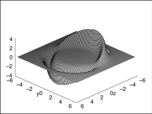
Figure 1: The expansion of the volume elements. These are expanding behind the spaceship, and contracting in front of it.

Note that the spaceship moves along a timelike curve, regardless of the value of $v(t)$. To verify this statement we simply substitute $z=z_{0}(t)$ in the metric, eq.$(1)$, which reduces to:

$$d\tau=dt$$ (3)

From which we conclude that the proper time equals the coordinate time, therefore the spaceship suffers no time dilation effects during it’s motion. It is also not difficult to prove that the spaceship moves along a geodesic.

2.2 Superluminal travel in the warp drive

To demonstrate that it is possible to travel to a distant point and back in an arbitrary short time interval, let us consider two distant stars, $A$ and $B$, separated by a distance $D$ in flat spacetime. Suppose that, at the instant $t_{0}$, a spaceship initiates it’s movement using the engines, moving away from $A$ with a velocity $v<1$. It comes to rest at a distance $d$ from $A$. For simplicity, assume that $R\ll d\ll D$.

It is at this instant that the perturbation of spacetime appears, centered around the spaceship’s position. The perturbation pushes the spaceship away from $A$, rapidly attaining a constant acceleration, $a$. Half-way between $A$ and $B$, the perturbation is modified, so that the acceleration rapidly varies from $a$ to $-a$. The spaceship finally comes to rest at a distance, $d$, from $B$, in which the perturbation disappears. It then moves to $B$ at a constant velocity in flat spacetime. The return trip to $A$ is analogous.

If the variations of the acceleration are extremely rapid, the total coordinate time, $T$, in a one-way trip will be:

$$T=2\left(\frac{d}{v}+\sqrt{\frac{D-2d}{a}}\right)$$

The proper time of the stars are equal to the coordinate time, because both are immersed in flat spacetime. The proper time measured by observers within the spaceship is given by:

$$\tau=2\left(\frac{d}{\gamma v}+\sqrt{\frac{D-2d}{a}}\right)$$

with $\gamma=(1-v^{2})^{-1/2}$. The time dilation only appears in the absence of the perturbation, in which the spaceship is moving with a velocity $v$, using only it’s engines in flat spacetime.

Using $R\ll d\ll D$, we can then obtain the following approximation:

$$\tau\approx T\approx 2\sqrt{\frac{D}{a}}$$

We verify that $T$ can be made arbitrarily short, increasing the value of $a$. The spaceship may travel faster than the speed of light. However, it moves along a spacetime temporal trajectory, contained within it’s light cone, for light suffers the same distortion of spacetime Alcubierre .

2.3 The violation of the WEC

Given a stress energy tensor $T_{\mu\nu}$, and a timelike vector $U^{\mu}$, the WEC states:

$$T_{\mu\nu}U^{\mu}U^{\nu}\geq 0$$ (4)

This condition is equivalent to the assumption that any timelike observer measures a local positive energy density.

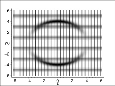
Figure 2: The negative energy density for a longitudinal cross section of the Alcubierre bubble. The energy density is distributed in a toroidal region perpendicular to the direction of travel. We have considered the following values: $v=2$, $\sigma=2$ and $R=8$.

We verify that for the warp drive metric, the WEC is violated:

$$T_{\mu\nu}U^{\mu}U^{\nu}=-\frac{1}{32\pi}\frac{v^{2}\rho^{2}}{r^{2}}\left(\frac{df}{dr}\right)^{2}<0$$ (5)

It is also possible to show that the dominant (DEC) and the strong energy condition (SEC) are also violated. In fig.$2$ we verify that the distribution of the negative energy density is concentrated in a toroidal region perpendicular to the direction of travel.

2.4 Interesting aspects of the Alcubierre spacetime

The Krasnikov analysis:

Krasnikov discovered a fascinating aspect of the warp drive, in which an observer on a spaceship cannot create nor control on demand an Alcubierre bubble, with $v>c$, around the ship Krasnikov . It is easy to understand this, as an observer at the origin (with $t=0$), cannot alter events outside of his future light cone, $|r|\leq t$, with $r=(\rho^{2}+z^{2})^{1/2}$. Applied to the warp drive, points on the outside front edge of the bubble are always spacelike separated from the centre of the bubble.

The analysis is simplified in the proper reference frame of an observer at the centre of the bubble. Using a transformation, $z^{\prime}=z-z_{0}(t)$, the metric is given by:

$$ds^{2}=-dt^{2}+d\rho^{2}+\rho^{2}d\phi^{2}+(dz^{\prime}+(1-f)vdt)^{2}$$ (6)

Consider a photon emitted along the $+Oz$ axis (with $ds^{2}=d\rho=0$):

$$\frac{dz^{\prime}}{dt}=1-(1-f)v$$ (7)

Initially, the photon has $\frac{dz^{\prime}}{dt}=1$ (because $f=1$ in the interior of the bubble). However, at some point $z^{\prime}=z^{\prime}_{c}$, with $f=1-\frac{1}{v}$, we have $\frac{dz^{\prime}}{dt}=0$ Everett . Once photons reach $z^{\prime}_{c}$, they remain at rest relative to the bubble and are simply carried along with it. This behaviour is reminiscent of an event horizon.

Reminiscence of an Event Horizon:

The appearance of an event horizon becomes evident in the 2-dimensional model of the Alcubierre space-time, with $\rho=0$ Hiscock ; Clark ; Gonz . The axis of symmetry coincides with the line element of the spaceship.

The metric, eq.$(1)$, reduces to :

$$ds^{2}=-(1-v^{2}f^{2})dt^{2}-2vfdzdt+dz^{2}$$ (8)

For simplicity, we consider the velocity of the bubble constant, $v(t)=v_{b}$. With $\rho=0$, we have $r=[(z-v_{b}t)^{2}]^{1/2}$. If $z>v_{b}t$, we consider the following transformation: $r=(z-v_{b}t)$. Note that the metric components of eq.$(8)$ only depend on $r$, which may be adopted as a coordinate.

Using the transformation, $dz=dr+v_{b}dt$, the metric, eq.$(8)$ is given by:

$$ds^{2}=-A(r)\left[dt-\frac{v_{b}(1-f(r))}{A(r)}dr\right]^{2}+\frac{dr^{2}}{A(r)}$$ (9)

The function $A(r)$, designated by the Hiscock function, is given by:

$$A(r)=1-v_{b}^{2}(1-f(r))^{2}$$ (10)

It’s possible to represent the metric, eq.$(9)$, in a diagonal form, using a new time coordinate:

$$d\tau=dt-\frac{v_{b}(1-f(r))}{A(r)}dr$$ (11)

with which eq.$(9)$ reduces to:

$$ds^{2}=-A(r)d\tau^{2}+\frac{dr^{2}}{A(r)}$$ (12)

This form of the metric is manifestly static. The $\tau$ coordinate has an immediate interpretation in terms of an observer on board of a spaceship: $\tau$ is the proper time of the observer, because $A(r)\rightarrow 1$ in the limit $r\rightarrow 0$.

We verify that the coordinate system is valid for any value of $r$, if $v_{b}<1$. If $v_{b}>1$, we have a coordinate singularity and an event horizon at the point $r_{0}$ in which $f(r_{0})=1-\frac{1}{v_{b}}$ and $A(r_{0})=0$.

3 The 2-dimensional Krasnikov solution

The Krasnikov metric has the interesting property that although the time for a one-way trip to a distant destination cannot be shortened, the time for a round trip, as measured by clocks at the starting point (e.g. Earth), can be made arbitrarily short, as will be demonstrated below.

The 2-dimensional metric is given by:

$$ds^{2}=-(dt-dx)(dt+k(t,x)dx)$$ (13)

where:

$$k(t,x)=1-(2-\delta)\theta_{\varepsilon}(t-x)\left[\theta_{\varepsilon}(x)-\theta_{\varepsilon}(x+\varepsilon-D)\right]$$ (14)

in which $\delta$ and $\varepsilon$ are arbitrarily small positive parameters. $\theta_{\varepsilon}$ denotes a smooth monotone function:

$$\theta_{\varepsilon}(\xi)=\left\{\begin{array}[]{ll}1,&{\rm if}\;\xi>\varepsilon,\\ 0,&{\rm if}\;\xi<0.\end{array}\right.$$

There are three distinct regions in the Krasnikov two-dimensional spacetime, which we shall summarize in the following manner.

The outer region: The outer region is given by the following set:

$$\{x<0\}\cup\{x>D\}\cup\{x>t\}$$ (15)

The metric is flat, $k=1$, and reduces to the Minkowski spacetime. Future light cones are generated by the vectors:

$$\left\{\begin{array}[]{ll}r_{O}=\partial_{t}+\partial_{x}\\ l_{O}=\partial_{t}-\partial_{x}.\end{array}\right.$$

The inner region: The inner region is given by the following set:

$$\{x<t-\varepsilon\}\cap\{\varepsilon<x<D-\varepsilon\}$$ (16)

This region is also flat, $k=\delta-1$, but the light cones are more open, being generated by the following vectors:

$$\left\{\begin{array}[]{ll}r_{I}=\partial_{t}+\partial_{x}\\ l_{I}=-(1-\delta)\partial_{t}-\partial_{x}.\end{array}\right.$$

The transition region: The transition region is a narrow curved strip in spacetime, with width $\sim\varepsilon$. Two spatial boundaries exist between the inner and outer regions. The first lies between $x=0$ and $x=\varepsilon$, for $t>0$. The second lies between $x=D-\varepsilon$ and $x=D$, for $t>D$. It is possible to view this metric as being produced by the crew of a spaceship, departing from point $A$ ($x=0$), at $t=0$, travelling along the $x$-axis to point $B$ ($x=D$) at a speed, for simplicity, infinitesimally close to the speed of light, therefore arriving at $B$ with $t\approx D$.

The metric is modified by changing $k$ from $1$ to $\delta-1$ along the $x$-axis, in between $x=0$ and $x=D$, leaving a transition region of width $\sim\varepsilon$ at each end for continuity. But, as the boundary of the forward light cone of the spaceship at $t=0$ is $|x|=t$, it is not possible for the crew to modify the metric at an arbitrary point $x$ before $t=x$. This fact accounts for the factor $\theta_{\varepsilon}(t-x)$ in the metric, ensuring a transition region in time between the inner and outer region, with a duration of $\sim\varepsilon$, lying along the wordline of the spaceship, $x\approx t$.

3.1 Superluminal travel within the Krasnikov tube

The properties of the modified metric with $\delta-1\leq k\leq 1$ can be easily seen from the factored form of $ds^{2}=0$. The two branches of the forward light cone in the $(t,x)$ plane are given by $\frac{dx}{dt}=1$ and $\frac{dx}{dt}=-k$.

The inner region, with $k=\delta-1$, is flat because the metric, eq.$(13)$, may be cast into the Minkowski form, applying the following coordinate transformations:

$$dt^{\prime}=dt+\left(\frac{\delta}{2}-1\right)dx$$ (17)

$$dx^{\prime}=\left(\frac{\delta}{2}\right)dx$$ (18)

The transformation is singular at $\delta=0$, i.e., $k=-1$. Note that the left branch of the region is given by $\frac{dx^{\prime}}{dt^{\prime}}=-1$.

From the above equations, one may easily deduce the following expression:

$$\frac{dt}{dt^{\prime}}=1+\left(\frac{2-\delta}{\delta}\right)\frac{dx^{\prime}}{dt^{\prime}}$$ (19)

For an observer moving along the positive $x^{\prime}$ and $x$ directions, with $\frac{dx^{\prime}}{dt^{\prime}}<1$, we have $dt^{\prime}>0$ and consequently $dt>0$, if $0<\delta\leq 2$. However, if the observer is moving sufficiently close to the left branch of the light cone, given by $\frac{dx^{\prime}}{dt^{\prime}}=-1$, eq.$(19)$ provides us with $\frac{dt}{dt^{\prime}}<0$, for $\delta<1$. Therefore $dt<0$, the observer traverses backward in time, as measured by observers in the outer region, with $k=1$.

The superluminal travel analysis is as follows. Imagine a spaceship leaving star $A$ and arriving at star $B$, at the instant $t\approx D$. The crew of the spaceship modify the metric, so that $k\approx-1$, for simplicity, along the trajectory.

Now suppose the spaceship returns to star $A$, travelling with a velocity arbitrarily close to the speed of light, i.e., $\frac{dx^{\prime}}{dt^{\prime}}\approx-1$. Therefore, from eqs$(17)$-$(18)$, one obtains the following relation:

$$v_{return}=\frac{dx}{dt}\approx-\frac{1}{k}=\frac{1}{1-\delta}\approx 1$$ (20)

and $dt<0$, for $dx<0$.

The return trip from star $B$ to $A$ is done in an interval of $\Delta t_{return}=-D/v_{return}=D/(\delta-1)$. The total interval of time, measured at $A$, is given by $T_{A}=D+\Delta t_{return}=D\delta$. For simplicity, consider $\varepsilon$ negligible.

Superluminal travel is implicit, because $|\Delta t_{return}|<D$, if $\delta>0$, i.e., we have a spatial spacetime interval between $A$ and $B$. Note that $T_{A}$ is always positive, but may attain a value arbitrarily close to zero, for an appropriate choice of $\delta$.

3.2 The 4-dimensional generalization

The metric in the 4-dimensional spacetime, written in cylindrical coordinates, is given by Everett :

$$ds^{2}=-dt^{2}+(1-k(t,x,\rho))dxdt+k(t,x,\rho)dx^{2}+d\rho^{2}+\rho^{2}d\phi^{2}$$ (21)

with:

$$k(t,x,\rho)=1-(2-\delta)\theta_{\varepsilon}(\rho_{max}-\rho)\theta_{\varepsilon}(t-x-\rho)[\theta_{\varepsilon}(x)-\theta_{\varepsilon}(x+\varepsilon-D)]$$ (22)

For $t\gg D+\rho_{max}$ one has a tube of radius $\rho_{max}$ centered on the $x$-axis, within which the metric has been modified. This structure is designated by the Krasnikov tube. In contrast with the Alcubierre spacetime metric, the metric of the Krasnikov tube is static once it has been created.

The stress-energy tensor element $T_{tt}$ given by:

$$T_{tt}=\frac{1}{32\pi(1+k)^{2}}\left[-\frac{4(1+k)}{\rho}\frac{\partial k}{\partial\rho}+3\left(\frac{\partial k}{\partial\rho}\right)^{2}-4(1+k)\frac{\partial^{2}k}{\partial\rho^{2}}\right]$$ (23)

can be shown to be the energy density measured by a static observer, and violates the WEC in a certain range of $\rho$, i.e, $T_{\mu\nu}U^{\mu}U^{\nu}<0$.

To verify the violation of the WEC, let us evaluate the energy density in the middle of the tube and at a time long after it’s formation, i.e., $x=D/2$ and $t\gg x+\rho+\varepsilon$, respectively. In this region we have $\theta_{\varepsilon}(x)=1$, $\theta_{\varepsilon}(x+\varepsilon-D)=0$ and $\theta_{\varepsilon}(t-x-\rho)=1$. With this simplification the form function, eq.$(22)$, reduces to:

$$k(t,x,\rho)=1-(2-\delta)\theta_{\varepsilon}(\rho_{max}-\rho)$$ (24)

Consider the following specific form for $\theta_{\varepsilon}(\xi)$ Everett :

$$\theta_{\varepsilon}(\xi)=\frac{1}{2}\left\{\tanh\left[2\left(\frac{2\xi}{\varepsilon}-1\right)\right]+1\right\}$$ (25)

so that the above form function is given by:

$$k=1-\left(1-\frac{\delta}{2}\right)\left\{\tanh\left[2\left(\frac{2\xi}{\varepsilon}-1\right)\right]+1\right\}$$ (26)

Choosing the following values for the parameters: $\delta=0.1$, $\varepsilon=1$ and $\rho_{max}=100\varepsilon=100$, the negative character of the energy density is manifest in the immediate inner vicinity of the tube wall, as shown in fig.$(3)$.

Figure 3: Graph of the energy density, $T_{tt}$, as a function of $\rho$ at the middle of the Krasnikov tube, $x=D/2$, and long after it’s formation, $t\gg x+\rho+\varepsilon$. We consider the following values for the parameters: $\delta=0.1$, $\varepsilon=1$ and $\rho_{max}=100\varepsilon=100$.

4 Superluminal travel requires the violation of the WEC

It is simpler to apply global techniques and the topology of space for a definition of superluminal travel. The following treatment is based on work by Ken Olum Olum .

A path, $P$, is defined along which a propagating signal travels further than a signal on any nearby path, in the same interval of externally defined time. Spacelike two-surfaces are constructed around the origin and destination points of the path, $P$. The spacetime metric is arranged so that a causal path exists between the origin and destination points, $A$ and $B$, respectively, but there are no other causal paths that connect the two-surfaces. Both two-surfaces, $\Sigma_{A}$ and $\Sigma_{B}$, are composed of a one-parameter family of spacelike geodesics through the respective origin and destination points.

Formally, a causal path, $P$, is superluminal from an origin point, $A$, to a destination point, $B$, only if it satisfies the following condition.

Superluminal Condition:

There exists 2-surfaces $\Sigma_{A}$ around $A$ and $\Sigma_{B}$ around $B$ such that:

$(i)$ if $p\in\Sigma_{A}$ then a spacelike geodesic lying in $\Sigma_{A}$ connects $A$ to $p$, and similarly for $\Sigma_{B}$, and,

$(ii)$ if $p\in\Sigma_{A}$ and $q\in\Sigma_{B}$, then $q\in J^{+}(p)$, i.e., $q$ is in the causal future of $p$, if and only if $p=A$ and $q=B$.

General considerations:

Let there be a path $P$ satisfying the above condition, and suppose that the generic condition holds on $P$ (recall that the generic condition states that the path $P$ contains a point in which $k_{[a}R_{b]cd[e}k_{f]}k^{c}k^{d}\neq 0$ is satisfied, where $k$ is the tangent vector to the geodesic). With these assumptions, it can be shown that the WEC must be violated, somewhere along $P$.

Note that $P$ must be a null geodesic.

Proof: If $P$ is not a geodesic it can be varied to make a timelike path from $A$ to $B$. Let $O$ be an open neighborhood of $B$ contained in $\Sigma_{B}$. If $P$ is timelike anywhere, then it can be varied to make a timelike path from $A$ to points of $O$ other than $B$, contradicting the Superluminal Condition.

Let $k$ be the tangent vector to the geodesic $P$. $k$ must be normal to the surface $\Sigma_{A}$, otherwise there would be points on $\Sigma_{A}$ in the past of points on $P$. Similarly for $\Sigma_{B}$.

We define a congruence of null geodesics with an affine parameter $u$, normal to $\Sigma_{A}$, and extend $k$ to be the tangent vector at each point of the congruence.

There is no point $x\in P$ that is conjugate to $\Sigma_{A}$.

Proof: If $x$ were an interior point of $P$ then it would be possible to deform $P$ into a timelike path Wald . If $x=B$, then different geodesics of the congruence would all end at $B$ or points in an open neighborhood close to $B$ contained in $\Sigma_{B}$. These geodesics would have different tangent vectors to $\Sigma_{B}$. Therefore no point on $P$ is conjugate to $\Sigma_{A}$.

The expansion of the geodesic congruence is given by $\hat{\theta}=k^{m}_{\;\;\;;m}$ , where $m$ runs over two orthogonal directions normal to $k$. At $A$ we use directions that lie in $\Sigma_{A}$ and at $B$ we use directions that lie in $\Sigma_{B}$. Since $\Sigma_{A}$ is extrinsically flat at $A$, the geodesics are initially parallel, therefore $\hat{\theta}=0$.

The evolution of the expansion, $\hat{\theta}$, is given by the Raychaudhuri equation for null geodesics:

$$\frac{d\hat{\theta}}{du}=-R_{\mu\nu}k^{\mu}k^{\nu}+2\hat{\omega}^{2}-2\hat{\sigma}^{2}-\frac{1}{2}\hat{\theta}^{2}$$ (27)

in which $\hat{\omega}$ is the twist, $\hat{\sigma}$ the shear and $R_{\mu\nu}$ is the Ricci tensor.

Since there are no conjugate points, $\hat{\theta}$ is well-defined along $P$. We also have $\hat{\omega}_{\mu\nu}=0$, because the congruence is (locally) hypersurface orthogonal, according to the dual formulation of Frobenius’ theorem Wald .

If the WEC holds, then by continuity the null energy condition (NEC) will also be satisfied. The NEC is given by $T_{\mu\nu}k^{\mu}k^{\nu}\geq 0$, for all null $k^{\mu}$. Using Einstein’s equation, we obtain $R_{\mu\nu}k^{\mu}k^{\nu}=8\pi T_{\mu\nu}k^{\mu}k^{\nu}$. Thus if the WEC is satisfied, then $R_{\mu\nu}k^{\mu}k^{\nu}\geq 0$ and therefore $\frac{d\hat{\theta}}{du}\leq 0$. From the generic condition, $k_{[a}R_{b]cd[e}k_{f]}k^{c}k^{d}\neq 0$ on a point along $P$, $\hat{\sigma}$ cannot vanish everywhere. Recall that $\hat{\theta}=0$ at $A$. Thus, the WEC implies, that at $B$, we have:

$$\hat{\theta}<0.$$ (28)

Weak energy condition violation:

If we can prove that the expansion obeys the inequality, $\hat{\theta}\geq 0$, at $B$, then the WEC is violated somewhere along $P$.

Firstly, it’s important to establish a basis for vectors at $B$. Let $E_{1}$ and $E_{2}$ be orthonormal vectors tangent to $\Sigma_{B}$ at $B$, and let $E_{3}$ be a unit spacelike vector orthonormal to $E_{1}$ and $E_{2}$, with $g(k,E_{3})>0$. Let $E_{4}$ be the unit future-directed timelike vector orthogonal to $E_{1}$, $E_{2}$ and $E_{3}$. Using this basis, normal Riemannian coordinates are established near $B$, so that the $2$-surface $\Sigma_{B}$ consists of points with $t=z=0$.

Let $\lambda(s)$ be a smooth curve on $\Sigma_{A}$, with $\lambda(0)=A$. Let $\lambda(s,u)$ be the point an affine distance $u$ along the null geodesic from $\lambda(s)$. Each geodesic will eventually pass near $B$ and will cross the hypersurface with $t=0$. This crossing point is called $\lambda^{\prime}(s)$, and the length of the vectors $k$ on $\Sigma_{A}$ are adjusted, so that $\lambda(s,1)=\lambda^{\prime}(s)$.

The $z$ coordinate of $\lambda^{\prime}(s)$ is negative, otherwise points on $\Sigma_{B}$ $(z=t=0)$ would be the future of points of the geodesics from $\Sigma_{A}$, contradicting the Superluminal Condition.

Let $Z$ be the tangent vector to $\lambda(s,u)$ in the $s$ direction. By construction, $k^{\mu}Z_{\mu}=0$ on $\Sigma_{A}$, which is constant along each geodesic Wald ; Hawking , so that $k^{\mu}Z_{\mu}=0$ is verified everywhere.

Following along $\lambda^{\prime}(s)$, from $B$, we have:

$$0=\frac{d}{ds}(k^{\mu}Z_{\mu})=(k^{\mu}Z_{\mu})_{;\nu}Z^{\nu}=k^{\mu}_{\;\;;\nu}Z_{\mu}Z^{\nu}+k^{\mu}Z_{\mu;\nu}Z^{\nu}$$ (29)

The only non-vanishing components of $k$ are $k^{3}$ and $k^{4}$. Since $\lambda^{\prime}(s)$ lies in the $t=0$ hypersurface, we have $Z^{4}=0$ everywhere, so that the only contribution to $k^{\mu}Z_{\mu;\nu}$ at $B$ is from $\mu=3$. Therefore, from the above relation, we have:

$$k^{\mu}_{\;\;;\nu}Z_{\mu}Z^{\nu}=-k^{3}Z_{3;\nu}Z^{\nu}$$ (30)

But at $B$, we have $Z_{3}=0$. We see that $Z_{3;\nu}Z^{\nu}\leq 0$, otherwise the $z$ coordinate of $\lambda^{\prime}(s)$ would become positive. By construction, $k^{3}>0$, so that $k^{3}Z_{3;\nu}Z^{\nu}\leq 0$ and $k^{\mu}_{\;\;;\nu}Z_{\mu}Z^{\nu}\geq 0$.

The congruence of geodesics provides a map from tangent vectors to $\lambda(s)$ at $A$ to tangent vectors to $\lambda^{\prime}(s)$ at $B$. As there are no conjugate points, the map is non-singular and can be inverted. Choices of $\lambda(s)$ can be found so that $Z=E_{1}$ or $Z=E_{2}$, thus $k^{1}_{\;\;;1}\geq 0$ and $k^{2}_{\;\;;2}\geq 0$, respectively, so that:

$$\hat{\theta}=k^{m}_{\;\;\;;m}\geq 0$$ (31)

contradicting $\hat{\theta}<0$.

Olum’s superluminal theorem:

Any spacetime that admits superluminal travel on some path $P$ (according to Olum’s definition of the Superluminal Condition) and that satisfies the generic condition on $P$, must also violate the WEC at some point of $P$.

4.1 Applications to the Casimir effect

It was already mentioned that although classical forms of matter obey the energy conditions, these are violated by certain quantum fields, amongst which we may refer to the quantized scalar and fermionic fields, the Casimir and the Topological Casimir Effect, squeezed vacuum states, the Hawking evaporation, the Hartle-Hawking vacuum, cosmological inflation, etc.

It is interesting to apply the Superluminal Condition to the Casimir effect Olum . The quantum expectation value of the electromagnetic stress-energy tensor between circular conducting plates is:

$$T_{\mu\nu}=\frac{\pi^{2}}{720d^{4}}diag(-1,1,1,-3)$$ (32)

For a geodesic travelling in the $z$-direction, we have:

$$R_{\mu\nu}k^{\mu}k^{\nu}=-\frac{2\pi^{2}}{45d^{4}}<0$$ (33)

Let $\Sigma_{A}$ be the lower plate and $\Sigma_{B}$ be the upper plate. Assuming that all the geodesics are initially parallel, so that $\hat{\theta}=0$ at $A$. We have $\hat{\sigma}=0$, by symmetry, and $\hat{\omega}=0$, because the congruence is hypersurface orthogonal. The Raychaudhuri equation reduces to:

$$\frac{d\hat{\theta}}{du}=-R_{\mu\nu}k^{\mu}k^{\nu}>0$$ (34)

This inequality shows that the geodesics around $P$ are defocused. Thus the geodesic $P$ travels further in the $z$-direction, by the same same $t$, than neighbouring geodesics, in which the Superluminal Condition is satisfied.

It is also important to note that the above analysis is probably not complete, because the mass of the plates have not been taken into account.

5 Quantum Inequality and applications

Intensive research has been going on into the violation of the energy conditions. It is interesting to note the pioneering work by Ford in the late 1970’s on a new set of energy constraints ford1 , which led to constraints on negative energy fluxes in 1991 ford2 . These eventually culminated in the form of the Quantum Inequality (QI) applied to energy densities, which was introduced by Ford and Roman in 1995 F&R1 .

The QI was proven directly from Quantum Field Theory, in four-dimensional Minkowski spacetime, for free quantized, massless scalar fields, and takes the following form:

$$\frac{\tau_{0}}{\pi}\int_{-\infty}^{+\infty}\frac{\langle{T_{\mu\nu}U^{\mu}U^{\nu}}\rangle}{\tau^{2}+{\tau^{2}_{0}}}d\tau\geq-\frac{3}{32\pi^{2}\tau^{4}_{0}},$$ (35)

in which, $U^{\mu}$ is the tangent to a geodesic observer’s wordline; $\tau$ is the observer’s proper time and $\tau_{0}$ is a sampling time. The expectation value $\langle\rangle$ is taken with respect to an arbitrary state $|\Psi\rangle$. One does not average over the entire wordline of the observer, as in the averaged energy conditions, but weights the integral with a sampling function of characteristic width, $\tau_{0}$. The inequalities limit the magnitude of the negative energy violations and the time for which they are allowed to exist. The basic applications to curved spacetimes is that these appear flat if restricted to a sufficiently small region.

Using the restrictions imposed by the QI to wormholes Roman and the warp drive PfenningF , it was verified that the throat size of the wormholes and the Alcubierre bubble wall are extremely thin, i.e., only slightly larger than the Planck length. It was also verified that the energy involved to support the Alcubierre bubble and the Krasnikov tube are probably not physically plausible, for they are extraordinary large. For example, considering the mass of a typical galaxy, $M_{MilkyWay}\approx 10^{12}M_{Sun}=2\times 10^{42}kg$, the energy necessary to support the Alcubierre bubble is $E\leq-5,5\times 10^{21}M_{MilkyWay}\times v_{b}$, which is of the order $10^{10}$ times the total mass of the Universe. In the opposite regime, for microscopic Alcubierre bubbles, of the order of the Compton length of an electron, the negative energy is of the order $E\sim-10^{4}M_{Sun}$. Due to these enormous amounts of exotic matter, van den Broeck proposed a slight modification of the Alcubierre metric which ameliorates considerably the conditions of the warp drive Broeck1 .

Considering the applications of the QI to the above-mentioned solutions, one may, rightly so, conclude that these solutions are not physically plausible. However, there are a series of considerations that can be applied to the QI Lobo . Firstly, the QI is only of interest if one is relying on quantum field theory to provide the exotic matter to support the solutions above-mentioned. But there are classical systems (non-minimally coupled scalar fields) that violate the null and the weak energy conditions B&V , whilst presenting plausible results when applying the QI. Secondly, even if one relies on quantum field theory to provide exotic matter, the QI does not rule out the existence of the considered solutions, although they do place serious constraints on the geometry.

Despite of the impressive work done by Ford and Roman, namely the deduction of the QI and all it s applications Everett ; Roman ; PfenningF ; PFord the current version of the QI is certainly not the last word on the subject of exotic matter and the energy condition violations.

6 Conclusion

It does seem to suggest that if one adopts a conservative view, and impose the WEC, Olum’s theorem prohibits superluminal travel. As was mentioned in the introduction the present work serves as a bridge to ongoing research on spacetimes which generate closed timelike curves. An extension of Olum’s theorem to these spacetimes is the next step, or the generalization and modification of his superluminal definition. This is not easily accomplished because most of the definitions adopted in the causal structure of spacetime Wald ; Hawking break down in the presence of CTCs.

References

- (1) M. Morris, K.S. Thorne: Wormholes in spacetime and their use for interstellar travel: A tool for teaching General Relativity, Am. J. Phys. 56, 395-412 (1988).
- (2) M. Visser: Lorentzian wormholes: From Einstein to Hawking (American Institute of Physics, New York, 1995).
- (3) M. Alcubierre: The Warp drive: hyper-fast travel within general relativity, Class. Quant. Grav. 11, L73-L77 (1994).
- (4) S.V. Krasnikov: Hyper-fast Interstellar Travel in General Relativity, Phys. Rev. D 57, 4760 (1998). gr-qc/9511068.
- (5) A.E. Everett, T.A. Roman: A Superluminal Subway: The Krasnikov Tube, Phys. Rev. D 56, 2100 (1997). gr-qc/9702049.
- (6) M. Visser, B. Bassett, S. Liberati: Perturbative superluminal censorship and the null energy condition, Proceedings of the Eighth Canadian Conference on General Relativity and Relativistic Astrophysics (AIP Press) (1999). gr-qc/9908023.
- (7) M. Visser, B. Bassett, S. Liberati: Superluminal censorship, Nucl. Phys. Proc. Suppl. 88, 267-270 (2000). gr-qc/9810026
- (8) K. Olum: Superluminal travel requires negative energy density, Phys. Rev. Lett, 81, 3567-3570 (1998). gr-qc/9805003.
- (9) L.H. Ford, T.A. Roman: Averaged energy conditions and quantum inequalities, Phys. Rev. D 51, 4277 (1995).
- (10) W.A. Hiscock: Quantum effects in the Alcubierre warp drive spacetime, Class. Quant. Grav. 14, L183 (1997). gr-qc/9707024.
- (11) C. Clark, W.A. Hiscock, S.L. Larson: Null geodesics in the Alcubierre warp drive spacetime: the view from the bridge, Class. Quant. Grav. 16, 3965 (1999). gr-qc/9907019.
- (12) P.F. González-Días: On the warp drive space-time (1999), gr-qc/9907026.
- (13) R.M. Wald: General Relativity (University of Chicago Press, Chicago, 1984).
- (14) S.W. Hawking, G.F.R. Ellis: The Large Scale Structure of Spacetime (Cambridge University Press, London, 1973).
- (15) L.H. Ford: Quantum coherence effects and the second law of thermodynamics, Proc. Roy. Soc. Lond. A 56, 227 (1978).
- (16) L.H. Ford: Constraints on negative-energy fluxes, Phys. Rev. D 43, 3972 (1991).
- (17) L.H. Ford, T.A. Roman: Quantum field theory constrains traversable wormhole geometries, Phys. Rev. D 53, 5496 (1999). gr-qc/9510071.
- (18) M.J. Pfenning, L.H. Ford: The unphysical nature of warp drive, Class. Quant. Grav. 14, 1743, (1997). gr-qc/9702026.
- (19) C. van den Broeck: A warp drive with more reasonable total energy requirements, Class. Quant. Grav. 16, 3973-3979, (1999). gr-qc/9905084.
- (20) F. Lobo, P. Crawford: Constraints on wormhole geometries, The Ninth Marcel Grossmann Meeting, Proceedings, Rome, Italy, 2000, edited by Vahe G. Gurzadyan, Robert Jantzen and Remo Ruffini (World Scientific, Singapore, 2002), 855-856.
- (21) C. Barcelo, M. Visser: Scalar fields, energy conditions, and traversable wormholes, Class. Quant. Grav. 17, 3843 (2000). gr-qc/0003025.
- (22) M.J. Pfenning, L.H. Ford: Quantum inequalities on the energy density in static Robertson-Walker spacetimes, Phys. Rev. D 55, 4813 (1997).