The Dynamics of Test Particles and Pointlike Gyroscopes
in the Brane World and Other 5D Models

Abstract

We study the dynamics of test particles and pointlike gyroscopes in 5D manifolds like those used in the Randall-Sundrum brane world and non-compact Kaluza-Klein models. Our analysis is based on a covariant foliation of the manifold using $3+1$ dimensional spacetime slices orthogonal to the extra dimension, and is hence similar to the ADM $3+1$ split in ordinary general relativity. We derive gauge invariant equations of motion for freely-falling test particles in the 5D and 4D affine parameterizations and contrast these results with previous work concerning the so-called “fifth force”. Motivated by the conjectured localization of matter fields on a 3-brane, we derive the form of the classical non-gravitational force required to confine particles to a 4D hypersurface and show that the resulting trajectories are geometrically identical to the spacetime geodesics of Einstein’s theory. We then discuss the issue of determining the 5D dynamics of a torque-free spinning body in the point-dipole approximation, and then perform a covariant $(3+1)+1$ decomposition of the relevant formulae (i.e. the 5D Fermi-Walker transport equation) for the cases of freely-falling and hypersurface-confined point gyroscopes. In both cases, the 4D spin tensor is seen to be subject to an anomalous torque. We solve the spin equations for a gyroscope confined to a single spacetime section in a simple 5D cosmological model and observe a cosmological variation of the magnitude and orientation of the 4D spin.

I Introduction

There has been a large amount of recent interest in the possibility that our world contains more than four non-compact dimensions. This interest has been largely motivated by the work of Randall and Sundrum (RS), who postulate that our 4D universe is in actuality a 3-brane moving in a higher dimensional manifold with large extra dimensions Randall and Sundrum (1999a, b). The introduction of such a model assists in the explanation of the hierarchy and cosmological constant problems. However, the existence of large extra dimensions raises several issues, not the least of which is the nature of the trajectories of test particles in a $(3+1)+d$ dimensional manifold. Several authors have considered this, both in the context of the $d=1$ brane world picture and non-compact 5D Kaluza-Klein theory. In the former scenario, matter is confined to the brane while gravitons are free to propagate in the bulk on 5D null geodesics. In the latter scenario, all particles travel on 5D geodesics but observers can only readily access the 4D part of the trajectory (Wesson, 1999, 2001, reviews). Specific topics tackled in the literature include deviations from 4D geodesic motion and the so-called “fifth force” Gross and Perry (1983); Cho and Park (1991); Mashhoon et al. (1998); Wesson et al. (1999); Youm (2000, 2001); Ponce de Leon (2001a, b), astrophysical and experimental tests of higher dimensional dynamics Kalligas et al. (1994); Wesson et al. (1997); Liu and Overdiun (2000), violations of 4D causality in the brane world Kalbermann and Halevi (1998); Kalbermann (2000); Chung and Freese (2000); Ishihara (2001), the tendency of the brane world to attract or repel buck geodesics Maartens (2000, 2001); Chamblin (2001), the subtle interplay between 4D and 5D affine parameters Chamberlin et al. (2000); Seahra and Wesson (2001), and the dynamical acquisition and variation of particle rest masses from dimensional reduction Mashhoon et al. (1994); Liu and Mashhoon (2000); Seahra and Wesson (2001); Billyard and Sajko (2001). In work closely related to the study of higher dimensional geodesics, several authors have considered the behaviour of pointlike gyroscopes moving in 5D manifolds Kalligas et al. (1994); Mashhoon et al. (1998); Liu and Overdiun (2000); Liu and Mashhoon (2000).

We will not address all of these issues in this paper. Rather, we present a generic formalism which may aid in the study of higher dimensional particle motion. In particular, we wish to describe the motion of test particles in a $(3+1)+1$ dimensional manifold in a geometric and covariant manner. Our approach is inspired by the familiar geometric construction used in the Arnowitt-Deser-Misner (ADM) Hamiltonian formulation of general relativity, where the 4D manifold is foliated by a series of 3D spacelike hypersurfaces $\Sigma_{t}$ Misner et al. (1970); Wald (1984). As described in detail in Section II, we introduce a similar foliation of the 5D manifold by a series of timelike 4D hypersurfaces $\Sigma_{\ell}$, each of which corresponds to a 4D spacetime. Here, $\ell$ labels the fifth dimension. The beauty of this approach is that it allows us to covariantly decompose 5D tensors in terms of quantities either tangent or orthogonal to $\Sigma_{\ell}$, and to derive equations that transform correctly under 4D and 5D coordinate changes.

Before describing our geometric framework in detail in Section II, we would like to outline the three main motivations for this work. First, we note that the majority of the references cited above deal with higher dimensional geodesics in 5D via the well known equation

$$\frac{d^{2}x^{A}}{d\lambda^{2}}+\Gamma^{A}_{BC}\frac{dx^{B}}{d\lambda}\frac{dx^{C}}{d\lambda}=0,$$ (1)

where $\lambda$ is a 5D affine parameter and $\Gamma^{A}_{BC}$ refers to the higher dimensional Christoffel symbols. Particle trajectories are decomposed into a 4D part by considering the $A=0,1,2,3$ components of (1) differently from the $A=4$ component, which governs the motion in the extra dimension. The 4D part can then be manipulated to look like the 4D equation of motion of a particle subjected to a non-gravitational acceleration; i.e. the “fifth force”. As pointed out by Ponce de Leon, this procedure has some drawbacks Ponce de Leon (2001a, b). The most serious one is that the algorithm is not covariant in 5D, which results in the gauge dependence of the extra force. Another problem is that the fifth force is not orthogonal to the 4-velocity, which contradicts standard 4D physics. To overcome these difficulties, Ponce de Leon has analyzed the 5D geodesic equation in terms of local basis vectors and introduced suitable redefinitions of various quantities to obtain a better-behaved description of test particle trajectories. We wish to present an alternative formalism based on a $(3+1)+1$ decomposition of the 5D geodesic equation that is more geometric than Ponce de Leon’s algorithm, yet still corrects the problems associated with descriptions based on (1). This is the subject of Section III.

The second goal of this paper is to explore the confinement of test particles to a given $\Sigma_{\ell}$ hypersurface. An essential ingredient of brane world models is that matter fields are confined to a 3-brane that is identified with our universe. In string theory, this confinement comes about naturally from strings with endpoints attached to the brane. In the RS picture, localization of the zero-mode of the graviton and other fields arises from the discontinuous nature of the geometry. Other authors have considered “smoothed-out” versions of the RS model by introducing finite-width, or “thick”, branes created via dynamical degrees of freedom Csaki et al. (2000); Emparan et al. (2000); Giovannini (2001); Rogatko (2001). Localization of gravity and other fields comes from a steep, but smoothly differentiable, extra-dimensional potential. In this paper, we aim to explore the classical analogue of these, and other, confinement mechanisms making use of the geometric framework discussed above. Several workers have both noted that in general, non-gravitational forces are required to keep test particles confined to a thin 3-brane Billyard and Coley (1997); Maartens (2000); Ishihara (2001). In Section IV, we will derive the general form of such a confining force for a 3-brane of arbitrary geometry and show that it is nothing but a generalization of the centripetal force from undergraduate mechanics.

Our final motivation comes from a result derived in Section IV, which states that test particles confined to a $\Sigma_{\ell}$ hypersurface by normal forces travel on geodesics of that hypersurface. This makes it impossible to distinguish certain higher dimensional scenarios from ordinary general relativity based on the kinematic data of test bodies. This causes us to search for another test for non-compact extra dimensions, namely the behaviour of pointlike gyroscopes in 5D manifolds. We extend previous work by describing the dynamics of a spinning body in terms of the foliation language of Section II and by considering both freely falling and confined gyroscopes. In Section V.1, we discuss the general formulation of the point gyroscope problem in 5D. In Section V.2, we apply our splitting algorithm to the spin equations of motion. In Section V.3, we discuss how our results should be interpreted in the presence of a thin 3-brane. Finally, in Section V.4, we give an example of how a point gyroscope behaves in a simple 5D cosmological setting. Our main result is that when observed in 4D, the spin angular momentum of a gyroscope confined to a $\Sigma_{\ell}$ hypersurface is not conserved and that the spin tensor will precess with respect to a 4D non-rotating frame due to the existence of an anomalous torque. Such effects may be observable by space-based experiments such as Gravity Probe B (Jantzen et al., 1996, review).

Our results are summarized in Section VI along with suggestions for future work.

Conventions

The 5D metric signature is $(+----)$ while the 4D metric signature is $(+---)$; i.e. the extra dimension is assumed to be spacelike. In this paper, uppercase Latin indices run from 0 – 4 and lowercase Greek indices run 0 – 3. Early lowercase Latin indices run over all four spatial dimensions 1 – 4, while late indices run over the three spatial dimensions 1 – 3 associated with the 4D manifold.

II Geometric Construction

In this section, we introduce our foliation of the 5D manifold and the various geometric quantities that figure prominently in subsequent calculations. Consider a 5D manifold $(M,g_{AB})$ with one timelike dimension and covered by an arbitrary system of coordinates $x^{A}$. We introduce a scalar function

$$\ell=\ell(x^{A}),$$ (2)

which is defined everywhere on $M$. The 4D hypersurfaces $\ell$ = constant, which we shall denote by $\Sigma_{\ell}$, are assumed to have a spacelike normal vector field given by

$$n_{A}=\Phi\partial_{A}\ell,\quad n^{A}n_{A}=-1.$$ (3)

Each of the $\Sigma_{\ell}$ hypersurfaces may be associated with a 3+1 dimensional spacetime. The scalar $\Phi$ which normalizes $n^{A}$ is known as the lapse function. We define the projection tensor as

$$h_{AB}=g_{AB}+n_{A}n_{B}.$$ (4)

This tensor is symmetric $h_{AB}=h_{BA}$ and orthogonal to $n_{A}$. We place a 4D coordinate system on each of the $\Sigma_{\ell}$ hypersurfaces $y^{\alpha}$. The four basis vectors

$$e^{A}_{\alpha}=\frac{\partial x^{A}}{\partial y^{\alpha}},\quad n_{A}e^{A}_{\alpha}=0$$ (5)

are by definition tangent the $\Sigma_{\ell}$ hypersurfaces and orthogonal to $n^{A}$. It is easy to see that $e^{A}_{\alpha}$ behaves as a 5D contravariant vector under 5D coordinate transformations $x^{A}\rightarrow\bar{x}^{A}$ and a 4D covariant vector under 4D coordinate transformations $y^{\alpha}\rightarrow\bar{y}^{\alpha}$. We can use these basis vectors to project 5D objects onto $\Sigma_{\ell}$ hypersurfaces. For example, for an arbitrary 5D covariant vector

$$T_{\alpha}=e_{\alpha}^{A}T_{A}.$$ (6)

Here, $T_{\alpha}$ is said to be the projection of $T_{A}$ onto $\Sigma_{\ell}$. Clearly, $T_{\alpha}$ behaves as a scalar under 5D coordinate transformations and a covariant vector under 4D transformations. The induced metric on the $\Sigma_{\ell}$ hypersurfaces is given by

$$h_{\alpha\beta}=e^{A}_{\alpha}e^{B}_{\beta}g_{AB}=e^{A}_{\alpha}e^{B}_{\beta}h_{AB}.$$ (7)

Just like $g_{AB}$, the induced metric has an inverse

$$h^{\alpha\gamma}h_{\gamma\beta}=\delta^{\alpha}_{\beta}.$$ (8)

The induced metric and its inverse can be used to raise and lower indices of 4-tensors and change the position of the spacetime index of the $e^{A}_{\alpha}$ basis vectors. This then implies

$$e_{A}^{\alpha}e^{A}_{\beta}=\delta^{\alpha}_{\beta}.$$ (9)

Also note that since $h_{AB}$ is entirely orthogonal to $n^{A}$, we can express it as

$$h_{AB}=h_{\alpha\beta}e^{\alpha}_{A}e^{\beta}_{B}.$$ (10)

We will also require an expression that relates 5D covariant derivative of 5-tensors to the 4D covariant derivative of the corresponding 4-tensors. For covariant 5-vectors, the appropriate formula is

$$\nabla_{\beta}T_{\alpha}=e^{B}_{\beta}e^{A}_{\alpha}\nabla_{B}(h_{A}{}^{C}T_{C}),$$ (11)

where $\nabla_{B}$ is the 5D covariant derivative on $M$ defined with respect to $g_{AB}$ and $\nabla_{\beta}$ is the 4D covariant derivative defined with respect to $h_{\alpha\beta}$. The generalization to tensors of higher rank is obvious. It is not difficult to confirm that this definition of $\nabla_{\alpha}$ satisfies all the usual requirements imposed on the covariant derivative operator.

At this juncture, it is convenient to introduce our definition of the extrinsic curvature $K_{\alpha\beta}$ of the $\Sigma_{\ell}$ hypersurfaces:

$$K_{\alpha\beta}=e^{A}_{\alpha}e^{B}_{\beta}\nabla_{A}n_{B}=\tfrac{1}{2}e^{A}_{\alpha}e^{B}_{\beta}\pounds_{n}h_{AB}.$$ (12)

Note that the extrinsic curvature is symmetric (i.e. $K_{\alpha\beta}=K_{\beta\alpha}$) and may be thought of as the derivative of the induced metric in the normal direction. This 4-tensor will appear often in what follows.

Finally, we note that $(y^{\alpha},\ell)$ defines an alternative coordinate system to $x^{A}$. The appropriate diffeomorphism is

$$dx^{A}=e_{\alpha}^{A}dy^{\alpha}+\ell^{A}d\ell,$$ (13)

where

$$\ell^{A}=\left(\frac{\partial x^{A}}{\partial\ell}\right)_{y^{\alpha}=\mathrm{const.}}$$ (14)

is the vector tangent to lines of constant $y^{\alpha}$. We can always decompose 5D vectors into the sum of a part tangent to $\Sigma_{\ell}$ and a part normal to $\Sigma_{\ell}$. For $\ell^{A}$ we write

$$\ell^{A}=N^{\alpha}e_{\alpha}^{A}-\Phi n^{A}.$$ (15)

This is consistent with $\ell^{A}\partial_{A}\ell=1$, which is required by the definition of $\ell^{A}$, and the definition of $n^{A}$. The 4-vector $N^{\alpha}$ is called the shift vector and it describes how the $y^{\alpha}$ coordinate system changes as one moves from a given $\Sigma_{\ell}$ hypersurface to another. Using our formulae for $dx^{A}$ and $\ell^{A}$, we can write the 5D line element as

$$d\mathcal{S}^{2} = g_{AB}\,dx^{A}dx^{B}$$ (16)

$$= h_{\alpha\beta}(dy^{\alpha}+N^{\alpha}d\ell)(dy^{\beta}+N^{\beta}d\ell)-\Phi^{2}\,d\ell^{2},$$

which reduces to $d\mathcal{S}^{2}=h_{\alpha\beta}dy^{\alpha}dy^{\beta}$ if $d\ell=0$.

This completes our description of the geometric structure we will use in the rest of the paper. We would like to stress that this formalism does not depend on the form of the higher dimensional field equations, or the choice of 5D or 4D coordinates. It is sufficiently general to be applied to a wide class of $(3+1)+1$ theories of gravity.

III Splitting of the 5D Geodesic Equation

III.1 5D Affine Parameterization

In this section, we utilize the formalism introduced above to split the 5D geodesic equation into a series of relations involving quantities that are either tangent or orthogonal to the $\Sigma_{\ell}$ hypersurfaces. The goal is to derive the 4D equation of motion, an equation governing the motion in the extra dimension, and an equation governing the norm of the 4-velocity.

We consider a 5D geodesic trajectory with 5-velocity $u^{A}$ satisfying

$$0 = u^{A}\nabla_{A}u^{B},$$ (17a)

$$\epsilon = u^{A}u_{A},$$ (17b)

with

$$u^{A}=\dot{x}^{A},$$ (18)

where an overdot denotes $D/d\lambda=u^{A}\nabla_{A}$ and $\epsilon=0,\pm 1$. Since the norm of $u^{A}$ is constant, $\lambda$ is an affine parameter. We define

$$\xi\equiv n_{A}u^{A},$$ (19)

which allows us to write

$$u^{A} = h^{AB}u_{B}-\xi n^{A}$$ (20a)

$$= e^{A}_{\alpha}u^{\alpha}-\xi n^{A}.$$ (20b)

using (4) and defining $u^{\alpha}=e^{\alpha}_{A}u^{A}$. Putting (20a) into (17a) and expanding yields

$$0=h^{AC}u_{C}\nabla_{A}(h^{BM}u_{M}-\xi n^{B})-\xi n^{A}\nabla_{A}u^{B}.$$ (21)

Contracting this with $e_{B}^{\beta}$ and using the fact that $h^{AC}=e^{A}_{\alpha}e^{C}_{\gamma}h^{\alpha\gamma}$ and $e_{B}^{\beta}n^{B}=0$, we get

$$u^{\alpha}\nabla_{\alpha}u^{\beta}=\xi(K^{\alpha\beta}u_{\alpha}+e^{\beta}_{B}n^{A}\nabla_{A}u^{B}),$$ (22)

where $K_{\alpha\beta}$ is defined by equation (12).

Returning to (17a) and (20a) we can write

$$0=(h^{AM}u_{M}-\xi n^{A})\nabla_{A}(h^{BC}u_{C})-u^{A}\nabla_{A}(\xi n^{B})$$ (23)

instead of (21). We can contract this with $n_{B}$ and use the facts that

$$0=h_{BC}n^{B}u^{C} \Rightarrow n_{B}\nabla_{A}(h^{BC}u_{C})=-h^{BC}u_{C}\nabla_{A}n_{B}$$

$$-1=n_{A}n^{A} \Rightarrow n_{B}\nabla_{A}n^{B}=0,$$

to obtain, after some algebra

$$\dot{\xi}=K_{\alpha\beta}u^{\alpha}u^{\beta}-\xi n^{A}u^{B}\nabla_{A}n_{B},$$ (24)

where we have noted that $\dot{\xi}=d\xi/d\lambda=u^{A}\nabla_{A}\xi$.

Continuing, we note that $\epsilon=g_{AB}u^{A}u^{B}$ can be expanded by making the substitution $g_{AB}=h_{\alpha\beta}e^{\alpha}_{A}e^{\beta}_{B}-n^{A}n^{B}$. The result is

$$\epsilon=h_{\alpha\beta}u^{\alpha}u^{\beta}-\xi^{2}.$$ (25)

In summary, equations (17) can be rewritten as

$$a^{\beta}(u) = \xi(K^{\alpha\beta}u_{\alpha}+e^{\beta}_{B}n^{A}\nabla_{A}u^{B}),$$ (26a)

$$\dot{\xi} = K_{\alpha\beta}u^{\alpha}u^{\beta}-\xi n^{A}u^{B}\nabla_{A}n_{B},$$ (26b)

$$\epsilon = h_{\alpha\beta}u^{\alpha}u^{\beta}-\xi^{2}.$$ (26c)

Here, we have defined the acceleration of a 4-vector by

$$a^{\beta}(q)\equiv q^{\alpha}\nabla_{\alpha}q^{\beta}.$$ (27)

It must be noted that these equations do not represent a strict $(3+1)+1$ splitting of the geodesic equation because the 5D vector $u^{A}$ appears on the righthand side of equations (26a) and (26b). This shortcoming can be easily alleviated by making use of (20b), but we find that the present form of the equations is more useful for subsequent calculations. We will therefore abstain from further manipulations.

As a consistency check, we can contract (26a) with $u_{\beta}$. After some algebra, we obtain

$$u^{\alpha}\nabla_{\alpha}(u^{\beta}u_{\beta})=2\xi(K_{\alpha\beta}u^{\alpha}u^{\beta}+h_{BC}u^{C}n^{A}\nabla_{A}u^{B}).$$ (28)

Substituting $h_{BC}=g_{BC}+n_{B}n_{C}$ and using equation (26c) yields after further manipulation

$$u^{\alpha}\nabla_{\alpha}\xi-\xi n^{A}\nabla_{A}\xi=K_{\alpha\beta}u^{\alpha}u^{\beta}-\xi n^{A}u^{B}\nabla_{A}n_{B}.$$ (29)

But, the lefthand side is easily seen to be equivalent to $u^{A}\nabla_{A}\xi=\dot{\xi}$. Hence, it is possible to derive equation (26b) from equations (26a) and (26c). Therefore, equations (26) are mutually consistent in that one of the set is redundant.

In conclusion, we have succeeded in splitting the 5D geodesic equation (17a) into an equation of motion for the 4-velocity (26a) and an equation governing motion in the extra dimension (26b). We have also rewritten the 5D affine parameter condition (17b) in a matter consistent with the $(3+1)+1$ split (26c).

III.2 Parameter Transformation to 4D Proper Time

Upon examination of equations (26), it becomes clear that the 5D affine parameter $\lambda$ cannot be the same as what is usually called the 4D proper time $s$. The reason is that the norm of the 4-velocity $u^{\alpha}$ is not equal to unity by equation (26c). In this section, we will detail a parameter transformation from the 5D affine parameter $\lambda$ to the 4D proper time $s$ that will make the norm of the 4-velocity constant.

Our parameter transformation is described by the following formulae:

$$u^{A}=\psi v^{A},\quad\psi=\frac{ds}{d\lambda},\quad v^{A}=\frac{dx^{A}}{ds}.$$ (30)

$v^{A}$ is the 5-velocity of the test particle in the $s$-parameterization. We need to also define

$$\chi=n^{A}v_{A}\Rightarrow\xi=\chi\psi.$$ (31)

The equation on the right follows from $\xi=n^{A}u_{A}$. We can substitute these expressions into equations (26) in order to see what the $(3+1)+1$ split of the geodesic equation looks like in the $s$ parameterization. After a straightforward, but tedious, calculation, we obtain

$$v^{\alpha}\nabla_{\alpha}v^{\beta} = \chi(K^{\alpha\beta}v_{\alpha}+e^{\beta}_{B}n^{A}\nabla_{A}v^{B})$$ (32a)

$$-v^{\beta}(\ln\psi)^{\prime},$$

$$d(\chi\psi)/ds = \psi(K_{\alpha\beta}v^{\alpha}v^{\beta}-\chi n^{A}v^{B}\nabla_{A}n_{B}),$$ (32b)

$$\epsilon = \psi^{2}(h_{\alpha\beta}v^{\alpha}v^{\beta}-\chi^{2}).$$ (32c)

Here, a prime ^′ denotes $D/ds=v^{A}\nabla_{A}$. In order to go further, we need to demand that the norm of the 4-velocity be unity in the proper time parameterization:

$$1 = h_{\alpha\beta}v^{\alpha}v^{\beta},$$ (33a)

$$\epsilon = \psi^{2}(1-\chi^{2}),$$ (33b)

where the bottom equation follows from (32c). We can use (33b) to show $(\chi\psi)^{\prime}=\psi^{\prime}/\chi$, which may then be substituted into equation (32b) to isolate $(\ln\psi)^{\prime}$. The resulting formula can then be inserted into (32a). This penultimate expression may be simplified by the use of the identity

$$\chi n^{A}v^{B}\nabla_{A}n_{B}=-h_{BC}n^{A}v^{C}\nabla_{A}v^{B},$$ (34)

which is obtained by operating $n^{A}\nabla_{A}$ on both sides of $1=h_{BC}v^{B}v^{C}$ and then using equation (4). We finally get the following expression for the 4-acceleration of $v^{\alpha}$:

$$a^{\beta}(v) = \chi\Big{[}(K^{\alpha\beta}v_{\alpha}-K_{\mu\nu}v^{\mu}v^{\nu}v^{\beta})+$$ (35)

$$(e_{B}^{\beta}-e_{B}^{\gamma}v_{\gamma}v^{\beta})n^{A}\nabla_{A}v^{B}\Big{]}.$$

Note that this acceleration is orthogonal to $v^{\alpha}$,

$$v_{\beta}a^{\beta}(v)=0,$$ (36)

which also follows from $v^{\alpha}v_{\alpha}=1$. This is in contrast to 5D affine parameterization, which has

$$u_{\beta}a^{\beta}(u)\neq 0.$$ (37)

That is, in the proper time parameterization the 4-acceleration is orthogonal to the 4-velocity, while in the 5D affine parameterization the 4-acceleration has components parallel to the 4-velocity.

To complete our discussion of the proper time parameterization, we need to specify how the velocity along the extra dimension $\chi$ evolves with $s$. Going back to equation (33b), it is clear that if $\epsilon=0$ then $\chi=\pm 1$. That is, if the 5D path is null, we must have $n^{A}v_{A}=\pm 1$. It is interesting to note that even if the 5D path is a null geodesic with $v^{A}v_{A}=0$, we can still have the 4D trajectory as timelike with $v^{\alpha}v_{\alpha}=1$. This correspondence between massless trajectories in 5D and massive ones in 4D has been noted before Seahra and Wesson (2001); Billyard and Sajko (2001); Youm (2001). For cases where $\epsilon=\pm 1$, we can use (33b) to get $(\chi\psi)^{\prime}=\psi\chi^{\prime}/(1-\chi^{2})$. This into (32b) gives

$$\chi^{\prime} = (1-\chi^{2})(K_{\alpha\beta}v^{\alpha}v^{\beta}-\chi n^{A}v^{B}\nabla_{A}n_{B}),\quad\epsilon=\pm 1,$$

$$\chi = \pm 1,\quad\epsilon=0.$$ (38)

These formulae, along with (35) and equations (33) give our description of the $(3+1)+1$ split of the 5D geodesic equation in the proper time parameterization.

III.3 Differences between the current formalism and the literature

Before discussing the confinement of particle trajectories to a given hypersurface, we shall discuss some of what makes the current work different from previous studies. As mentioned in Section I, a number of authors have considered the force-free motion of particles in 5D, but most have concentrated on the determination of equations of motion from (1) or the equivalent variational principle (Wesson, 2001, references therein). The splitting of spacetime from the extra coordinate has been achieved by considering the first four equations of motion differently from the last one. The algorithm presented in Section III achieves the splitting in a more geometric fashion, employing the $(3+1)+1$ dimensional foliation technology introduced in Section II. This fundamental difference in methodology results in two main differences between descriptions of 5D geodesics. We proceed to outline these differences in this section.

First, we note that the central object in our description of particle trajectories is $u^{\alpha}=e^{\alpha}_{A}u^{A}$ while in the literature it is $\dot{y}^{\alpha}=dy^{\alpha}/d\lambda$. But these are not equal. To see this, we can use equations (13), (15) and (18) to get

$$u^{A}=e^{A}_{\alpha}(\dot{y}^{\alpha}+\dot{\ell}N^{\alpha})-\Phi\dot{\ell}n^{A}.$$ (39)

This then yields

$$u^{\alpha} = \dot{y}^{\alpha}+\dot{\ell}N^{\alpha},$$ (40a)

$$\xi = \Phi\dot{\ell}.$$ (40b)

These equations essentially replace equation (18) in the same manner that equations (26) replace equations (17). The important thing to note is that $u^{\alpha}$ is not equal to $dy^{\alpha}/d\lambda$, as may naïvely be assumed. We can understand equation (40a) by interpreting it as an equation concerning relative velocities. Geometrically, equation (14) tells us that the $\dot{\ell}N^{\alpha}$ term in (40a) represents the projected velocity of points on the $y^{\alpha}$ coordinate grid with respect to a “stationary” coordinate frame $\bar{y}^{\alpha}$ (i.e. a system of coordinates on $\Sigma_{\ell}$ with $N^{\alpha}=0$). This stationary coordinate frame has been extensively studied in the literature and has been termed “canonical” Mashhoon et al. (1998); Seahra and Wesson (2001); Billyard and Sajko (2001). Obviously, $\dot{y}^{\alpha}$ is the 4-velocity of the particle with respect to the $y^{\alpha}$ grid. Therefore, $u^{\alpha}$ is the velocity of the particle with respect to the $\bar{y}^{\alpha}$ frame, or, in other words, the velocity of the particle in canonical coordinates. The fact that $u^{\alpha}\neq\dot{y}^{\alpha}$ is not particularly worrisome because having solved equations (26) it is easy to obtain $\dot{y}^{\alpha}$ and $\dot{\ell}$ from equations (40).

The second way in which the results of Sections III.1 and III.2 differ from previous studies has to do with the presentation of the equations of motion. In the literature, higher dimensional geodesics are often analyzed in terms of the so-called “fifth force”, which for any 4-vector $q^{\alpha}$ is defined as

$$f^{\alpha}(q)=\frac{dq^{\alpha}}{d\lambda}+\Gamma^{\alpha}_{\beta\gamma}q^{\beta}q^{\gamma},$$ (41)

where $\Gamma^{\alpha}_{\beta\gamma}$ are the Christoffel symbols associated with $h_{\alpha\beta}$. In 4D, $f^{\alpha}(q)$ is identical to the acceleration of $q^{\alpha}$. However, the equality between $f^{\alpha}(q)$ and $a^{\alpha}(q)$ does not hold in 5D. To see this, we write

$$f^{\alpha}(q) = q^{A}\partial_{A}q^{\alpha}+\Gamma^{\alpha}_{\beta\gamma}q^{\beta}q^{\gamma}$$ (42)

$$= (h^{AB}-n^{A}n^{B})q_{A}\partial_{B}q^{\alpha}+\Gamma^{\alpha}_{\beta\gamma}q^{\beta}q^{\gamma}$$

$$= q^{\beta}\partial_{\beta}q^{\alpha}+\Gamma^{\alpha}_{\beta\gamma}q^{\beta}q^{\gamma}-(q_{A}n^{A})n^{B}\partial_{B}q^{\alpha}$$

$$= q^{\beta}\nabla_{\beta}q^{\alpha}-(q_{A}n^{A})n^{B}\partial_{B}q^{\alpha}.$$

In going from the second to the third line, we have used the fact $e^{B}_{\beta}\partial_{B}=\partial_{\beta}$ after making the substitution $h^{AB}=h^{\alpha\beta}e^{A}_{\alpha}e^{B}_{\beta}$. We have therefore established that fifth force is not equal to the 4D acceleration vector, instead they are related via

$$f^{\alpha}(q)=a^{\alpha}(q)-(q_{B}n^{B})n^{A}\partial_{A}q^{\alpha}.$$ (43)

This equation raises an important point about the behaviour of $f^{\alpha}$ under 4D coordinate transformations. It is obvious from equation (27) that $a^{\alpha}(q)$ is a 4-vector. But we will now demonstrate that $-\xi n^{A}\partial_{A}q^{\alpha}$ is not. Consider a 4D coordinate transformation $y^{\alpha}\rightarrow\tilde{y}^{\alpha}$. Under such a transformation, we know that $q^{\alpha}$ transforms as a 4-vector: $\tilde{q}^{\alpha}=(\partial\tilde{y}^{\alpha}/\partial y^{\beta})q^{\beta}$. This implies the following transformation law for $n^{A}\partial_{A}q^{\alpha}$:

$$n^{A}\partial_{A}\tilde{q}^{\alpha}=\frac{\partial\tilde{y}^{\alpha}}{\partial y^{\beta}}n^{A}\partial_{A}q^{\beta}+\frac{q^{\beta}}{\Phi}\left(N^{\mu}\partial_{\mu}-\partial_{\ell}\right)\frac{\partial\tilde{y}^{\alpha}}{\partial y^{\beta}}.$$ (44)

Here, we have used equation (15) to substitute for $n^{A}$ and then the definitions of $e^{A}_{\alpha}$ and $\ell^{A}$ with the chain rule to transform the partial derivatives. The first term on the RHS is what one would expect to see if $n^{A}\partial_{A}q^{\alpha}$ was indeed a 4-vector. But the presence of the second term indicates that it is not. In particular, if either the shift vector $N^{\alpha}$ is nonzero or the 4D coordinate transformation depends on $\ell$, then $n^{A}\partial_{A}q^{\alpha}$ will not satisfy the usual tensor transformation law. This of course means that the fifth force defined by (41) is not a 4-vector. Also, we note that several authors have found that in the $s$-parameterization the fifth force is not orthogonal to 4-velocity, which is in direct contradiction with standard 4D physics. This difficulty is removed by adopting the description of Section III.2, where the acceleration of $v^{\alpha}$ is properly orthogonal to $v^{\alpha}$. For these two reasons, we prefer to describe the 5D geodesics in terms of $a^{\alpha}$ as opposed to $f^{\alpha}$. This choice is not critical because one can easily move between the two descriptions by using equation (43).

IV Confinement of trajectories to $\Sigma_{\ell}$ hypersurfaces

As mentioned in Section I, a variety of different mechanisms have been suggested to confine matter fields to a 3-brane. In this section, we explore the classical particle analogue of this field concept. Our goal is to find out what kind of force per unit mass is required to confine test particles to a given $\Sigma_{\ell}$ hypersurface, and to determine the form of the 4D equation of motion. Our description is essentially that of an effective theory, since we do not speculate about the source of this non-gravitational acceleration. In what follows, we will use the term force to refer to what should properly be called a force per unit mass.

There are several possible avenues one can use to derive the confinement force. One possibility is to modify the calculation of Section III.1 to include an undetermined external force. Then, one can enforce the confinement of the particle by demanding $\xi=0$, which in turn places constraints on the external force. Another route begins with the Gauss-Weingarten equation, which relates the 4D and 5D accelerations of a curve confined to a given $\Sigma_{\ell}$ hypersurface, and can hence be used to fix the form of the non-gravitational force Misner et al. (1970); Ishihara (2001). However, if one wishes to proceed from first principles, a particularly transparent derivation comes from the method of Lagrange multipliers, which is what we will give in this section.

We take the 5D particle Lagrangian, in the affine parameterization, to be

$$\mathcal{L}=\tfrac{1}{2}g_{AB}u^{A}u^{B}+\mu(\lambda)\Phi(\lambda)\left[\ell(x^{N})-\ell_{0}\right].$$ (45)

Here, the constraint on the particle motion is given by $\varphi(x^{A})=\ell(x^{A})-\ell_{0}=0$, which essentially means that the trajectory is confined to the $\Sigma_{\ell}$ hypersurface corresponding to $\ell(x^{A})=\ell_{0}$. The undetermined function $\mu(\lambda)$ is the Lagrange multiplier. We have factored out a $\Phi(\lambda)$ term, which is the lapse function evaluated along the trajectory. We have done this to simplify the equations of motion, which are obtained from the standard Euler-Lagrange formulae. This result is

$$u^{B}\nabla_{B}u^{A}=\mu n^{A},$$ (46)

where we have used $n_{A}=\Phi\partial_{A}\ell$. Now, because $\varphi=0$ along the trajectory, we require that $u^{A}\partial_{A}\varphi=0$. This condition may be written as

$$0=\xi=u^{A}n_{A},$$ (47)

which is an obvious requirement for paths confined to a given $\Sigma_{\ell}$ hypersurface. We now contract both sides of (46) with $n_{A}$ and make use of the fact that (47) implies that $n_{A}\nabla_{B}u^{A}=-u^{A}\nabla_{B}n_{A}$ to obtain

$$\mu=u^{A}u^{B}\nabla_{A}n_{B}.$$ (48)

Finally, we note that since $\xi=0$ we can write $u^{A}=e^{A}_{\alpha}u^{\alpha}$, which yields that

$$\mu=K_{\alpha\beta}u^{\alpha}u^{\beta}.$$ (49)

This result fixes the force of constraint $\mu n^{A}$ that appears on the RHS of the equation of motion (46).

We now wish to address the issue of what happens to the $(3+1)+1$ splitting performed in Section III.1 in the presence of this confinement force. We can replace the ordinary geodesic equation (17a) with the constrained equation of motion (46) and our solution for $\mu$. Then, without first demanding that $\xi=0$, we can redo the manipulations of Section III.1 on the new equations. It transpires that equations (26a) and (26c) are unaffected by the presence of the confining force. However, equation (26b) is modified to read

$$\dot{\xi}=-\xi n^{A}u^{B}\nabla_{A}n_{B}.$$ (50)

One possible solution to the modified system of equations formed by (26a), (26c), and (50) is $\xi=0$. Assuming that we do have a situation where $\xi=0$, then spilt geodesic equations of motion given by (26) become

$$u^{\beta}\nabla_{\beta}u^{\alpha}=0,\quad\xi=0,\quad\epsilon=h_{\alpha\beta}u^{\alpha}u^{\beta}.$$ (51)

In other words, we have discovered that if the higher dimensional equation of motion is given by

$$u^{B}\nabla_{B}u^{A}=(K_{\alpha\beta}u^{\alpha}u^{\beta})n^{A},$$ (52)

and we impose the initial condition $\xi=0$, then the particle trajectory will be confined to a single $\Sigma_{\ell}$ hypersurface. In addition, the particle will travel on a 4D geodesic of that hypersurface, defined by $u^{\beta}\nabla_{\beta}u^{\alpha}=0$ and $u^{\alpha}u_{\alpha}=\epsilon$. In more physical terms, we can say that motion of the particle under the action of the 5D confinement force looks like force-free 4D motion on $\Sigma_{\ell}$.

This conclusion merits a few comments before we move on to the next section. First, the form of the confinement force could have been anticipated from elementary physics. Although our formulae have been derived with a 5D manifold in mind, they hold equally well in any dimension. So, consider a 2+1 dimensional flat manifold in polar coordinates with a line element

$$ds^{2}=dt^{2}-dr^{2}-r^{2}d\phi^{2}.$$ (53)

Suppose that in this manifold there is a particle confined to move on an $r=R$ hypersurface; i.e. on a circle of radius $R$. Then, the force per unit mass constraining the trajectory has a magnitude of $|K_{\alpha\beta}u^{\alpha}u^{\beta}|=R(d\phi/ds)^{2}=v^{2}/R$, where $v=R\,d\phi/ds$ is the linear spatial velocity. This result is recognized as the centripetal acceleration of a particle moving in a circle from undergraduate mechanics. Therefore, the confinement force we have derived in this section is nothing more than the higher dimensional generalization of the familiar centripetal acceleration.

Second, the causal properties of the 5D trajectories are preserved when they are confined to 4D hypersurfaces. This is, the fact that $u^{A}u_{A}=u^{\alpha}u_{\alpha}=\epsilon$ implies that timelike paths in 5D remain timelike when confined to $\Sigma_{\ell}$, null paths in 5D remain null when confined to $\Sigma_{\ell}$, etc…. This is contrast with Section III.2, where we saw that the projection of a 5D null geodesic path onto a $\Sigma_{\ell}$ hypersurface could be timelike, but with a complicated equation of motion (35). In other words, free massless particles in 5D can look like accelerated massive particles in 4D, but confined massless particles in 5D look like free massless particles in 4D. On a related note, the 5D affine parameter $\lambda$ coincides with the 4D proper time $s$ for confined paths.

The third point is that the confining force vanishes if $K_{\alpha\beta}=0$. In this case, geodesics on $\Sigma_{\ell}$ are automatically geodesics of the 5D manifold $M$. As pointed out by Ishihara, this is hardly a new result Ishihara (2001). Hypersurfaces that have $K_{\alpha\beta}=0$ are known as geodesically complete. However, it should be pointed out that $K_{\alpha\beta}=0$ is a sufficient, but not necessary condition for a geodesic on $\Sigma_{\ell}$ to also be a geodesic of $M$. The necessary condition is $K_{\alpha\beta}u^{\alpha}u^{\beta}=0$, which can be satisfied if $K_{\alpha\beta}\neq 0$. For example, the asymptotes of a hyperboloid $S$ in Euclidean 3-space are geodesics of both $S$ and $\mathbb{E}_{3}$. But, it is not difficult to show that if all the geodesics on $\Sigma_{\ell}$ are geodesics of $M$, then $K_{\alpha\beta}$ is necessarily zero.

Fourth, we should comment on how the calculations of this section fit into the brane world scenario. The observant reader will have already noticed that our manipulations implicitly assume that the 5D manifold is smooth and free of defects. Since this is not the case in the thin brane world scenario, one may legitimately wonder whether or not our results apply to a particle confined to a 3-brane. To answer the question, suppose that our 5D manifold contains a 3-brane corresponding to the $\Sigma_{\ell=0}=\Sigma_{0}$ hypersurface. We can view the trajectory of a confined particle on the brane $\gamma_{0}$ as the limit of a series of confined trajectories on hypersurfaces living in the bulk. To have a sensible theory, the limiting procedure must result in the same $\gamma_{0}$ curve as the brane is approached from the $\ell>0$ and $\ell<0$ sides. Now, consider the curves $\gamma_{\pm}$ located on the hypersurfaces $\Sigma_{\pm}$ at $\ell=0^{\pm}$. Since the $\Sigma_{\pm}$ hypersurfaces are in the bulk, $\gamma_{\pm}$ satisfy equations (51) with $h_{\alpha\beta}\rightarrow h_{\alpha\beta}^{\pm}$. But one of Israel’s junction conditions, which must be satisfied in the neighborhood of the brane, is

$$[h_{\alpha\beta}]=0,$$ (54)

where we have used the usual jump notation: $[(\cdots)]=(\cdots)_{\ell=0^{+}}-(\cdots)_{\ell=0^{-}}$. That is, the intrinsic 4-geometry of the $\Sigma_{\ell}$ hypersurfaces must be continuous across the brane. Since the confined trajectories $u^{A}_{\pm}$ are determined entirely by the intrinsic geometry, we see that both $\gamma_{+}$ and $\gamma_{-}$ must approach $\gamma_{0}$ as $\ell\rightarrow 0$. Therefore, the confined trajectories on the brane are perfectly well defined and are described by (51). However, it is interesting to note that the acceleration of the $\gamma_{\pm}$ curves, as given in equation (52), will not be continuous across the brane. This is because of the $\mathbb{Z}_{2}$ symmetry of the brane world, which says the the extrinsic curvature of the $\Sigma_{\ell}$ hypersurfaces is discontinuous about $\ell=0$:

$$K_{\alpha\beta}^{+}=-K_{\alpha\beta}^{-}\Rightarrow[K_{\alpha\beta}]\neq 0.$$ (55)

Therefore, the 5D acceleration of $\gamma_{0}$ cannot be sensibly defined because the one-sided limits of $A^{B}=K_{\alpha\beta}u^{\alpha}u^{\beta}n^{B}$ do not agree. At this juncture, this is not a source of concern because $A^{B}$ is orthogonal to the brane and is hence not directly measurable by observers. However, we shall see below that this acceleration is measurable in a different context, which will necessitate careful consideration.

Our fifth, and final, point is that the 4D equation of motion $u^{\alpha}\nabla_{\alpha}u^{\beta}=0$ means that we cannot observationally distinguish between a purely 4D universe with potentially exotic matter and a brane world type scenario from the kinematic data of macroscopic test particles. In both cases, we have geodesic motion on the 4D manifold. If we want to determine if our world is fundamentally 4D or if we are merely confined to a 4D hypersurface, we need to introduce new concepts, which is the subject of the next section.

V 5D pointlike gyroscopes

V.1 A spinning particle in 5D

In Section IV, we saw that if a particle is confined to a $\Sigma_{\ell}$ hypersurface by a centripetal confinement force, then it will travel on a geodesic of $\Sigma_{\ell}$. This means that we cannot observationally distinguish between confined motion in 5D and free motion in 4D by studying the form of the trajectory $x^{\alpha}=x^{\alpha}(\lambda)$. However, just as an observer in a closed vessel can use a gyroscope to determine if he is in a rotating reference frame, we will see that we can use spinning bodies to determine if apparently free particles are in actuality accelerating in higher dimensions.

Our staring point is the equations of motion for a “point-dipole” spinning particle moving in a 5D manifold. These equations for force free motion in 4D given by Papapetrou Papapetrou (1951); Mashhoon (1971) and were later generalized by Schiff to include non-gravitational forces and pointlike gyroscopes Schiff (1960a, b). The extension to 5D is trivial, provided that we assume that any non-gravitational forces exert no torque on the body. The equation of motion for the anti-symmetric spin tensor $\sigma^{AB}$ is

$$\dot{\sigma}^{AB}=u^{B}u_{C}\dot{\sigma}^{AC}-u^{A}u_{C}\dot{\sigma}^{BC}.$$ (56)

Here, $u^{A}$ is the 5-velocity, and an overdot indicates $D/d\lambda=u^{A}\nabla_{A}$. The equation of motion for the 5-velocity is

$$u^{A}\nabla_{A}u^{B}=A^{B},\quad u^{A}u_{A}=1,$$ (57)

where $A^{B}$ is the 5D acceleration induced by non-gravitational forces. We have followed Schiff and neglected the coupling of the Riemann tensor to $u^{A}$ as is appropriate for a point gyroscope. We will apply equations (56) and (57) to 5D pointlike gyroscopes that are freely falling, as described in Section III.1, and gyroscopes that are subject to a centripetal confining force, as described in Section IV. In the latter case, we must assume that the confining force acts at the center of mass to satisfy the torque-free requirement. Essentially, we need to neglect the “tidal” variation in the confining force over the body, which is reasonable for a body of extremely small size. With these assumptions in mind, we can apply the above spin equations of motion to a pointlike gyroscope in 5D.

However, our analogy with familiar spacetime physics must end here because we cannot generalize the 4D procedure of mapping the spin tensor $\sigma^{AB}$ onto a unique spin vector $\sigma^{A}$ to the 5D case. To see why this is so, we note that contraction of equation (56) with $u^{A}$ reveals that four of the ten equations for $\dot{\sigma}^{AB}$ are redundant. Hence the system of equations (56) is underdetermined; that is, we need to impose some sort of subsidiary condition on $\sigma^{AB}$. As in 4D, we can choose the spin tensor to be orthogonal to the 5-velocity

$$\sigma^{AB}u_{A}=0.$$ (58)

This reduces the number of degrees of freedom in $\sigma^{AB}$ to six. The same requirement in 4D implies that the spin tensor has three independent components that can be uniquely mapped onto a 4-vector orthogonal to the 4-velocity. But in 5D, a 5-vector orthogonal to the 5-velocity has four components, which is not enough to describe $\sigma^{AB}$. But, the six degrees of freedom do correspond to the number of independent components of an antisymmetric 4-dimensional matrix. This motivates us to decompose $\sigma^{AB}$ into a basis $\{\sigma_{a}^{A}\}$ that spans the space orthogonal to $u^{A}$:

$$\sigma^{AB}=\sigma^{ab}\sigma_{a}^{A}\sigma_{b}^{B},\quad 0=u_{A}\sigma^{A}_{a},\quad\sigma^{ab}=-\sigma^{ba}.$$ (59)

We now demand that the $\{\sigma_{a}^{A}\}$ basis is chosen in a manner that ensures that the $4\times 4$ $\sigma^{ab}$ matrix has constant entries:

$$\nabla_{A}\sigma^{ab}=0.$$ (60)

Note that $\sigma^{ab}$ behaves like a 5D scalar quantity. Substitution of our assumed form of $\sigma^{AB}$ into equation (56) and contracting with $\sigma^{A}_{c}$ yields, after some algebra

$$0=\sigma^{ab}\left\{(\sigma_{a}\cdot\sigma_{c})[\dot{\sigma}_{b}+(\dot{u}\cdot\sigma_{b})u]+(\dot{\sigma}_{a}\cdot\sigma_{c})\sigma_{b}\right\},$$ (61)

where we have suppressed the 5D indices for clarity. This can be solved in a manner independent of our choice of $\sigma^{ab}$ if the basis vectors satisfy

$$u^{B}\nabla_{B}\sigma^{A}_{a}=-(A_{B}\sigma^{B}_{a})u^{A},$$ (62)

where we have made use of (57). This is the equation of 5D Fermi-Walker (FW) transport of $\sigma^{A}_{a}$ along the integral curves of $u^{A}$ subject to the condition $0=u_{A}\sigma^{A}_{a}$. Therefore, we have demonstrated that the spin tensor of a pointlike gyroscope in 5D can be expressed in the form given in equation (59), where $\sigma^{ab}$ is an arbitrary $4\times 4$ antisymmetric tensor with constant entries, provided that the $\{\sigma^{A}_{a}\}$ basis is FW transported along the gyroscope’s trajectory. The six degrees of freedom of $\sigma^{AB}$ are carried by the $\sigma^{ab}$ matrix.

We note that the spin vector of a particle in 4D is governed by an equation identical to (62). Therefore, the problem of determining the evolution of the spin tensor of a pointlike gyroscope in 4D and 5D is operationally identical; i.e. one needs to solve the FW transport equation. However, the relation between the solution(s) of that equation and the full spin tensor is different. It is interesting to note that the method outlined here will work in any dimension, including 3+1, while the procedure of identifying spin angular momentum with a single vector is peculiar to the case of three spatial dimensions. Regardless, we are now faced with the prospect of solving the FW equation in 5D. This is the subject of the next section.

V.2 Splitting of the 5D Fermi-Walker transport equation

In this section, we will attempt to perform a $(3+1)+1$ splitting of the equation of FW transport for the spin-basis vectors $\{\sigma^{A}_{a}\}$ similar to the splitting of the geodesic equation performed in Section III.1. The relevant formulae are given by equations (57) and (62). For brevity, we will omit the Latin index on the spin-basis vector $\sigma_{a}^{A}$. We will consider the cases of free and constrained motion in 5D by setting

$$A^{B}=\begin{cases}0,&\text{for 5D geodesic motion,}\\ K_{\alpha\beta}u^{\alpha}u^{\beta}n^{B},&\text{for 5D confined paths.}\end{cases}$$ (63)

As mentioned above, we assume that the spin basis is orthogonal to $u^{A}$. Since $\sigma^{A}$ is FW transported along the gyroscope trajectory, its magnitude is constant and can be set to $-1$. Hence we also have

$$u^{A}\sigma_{A}=0,\quad\sigma^{A}\sigma_{A}=-1.$$ (64)

We also define

$$\sigma^{\alpha}=e^{\alpha}_{A}\sigma^{A},\quad\varSigma=\sigma^{A}n_{A}.$$ (65)

Case 1: $A^{B}=0$.

The gyroscope’s center of mass motion is described by equations (26). The mechanics of the decomposition of equations (62) and (64) is similar to the calculations of Section III.1, so we will omit the details and present the final results. We get

$$u^{\alpha}\nabla_{\alpha}\sigma^{\beta} = \varSigma K^{\alpha\beta}u_{\alpha}+\xi e^{\beta}_{B}n^{A}\nabla_{A}\sigma^{B},$$ (66a)

$$\dot{\varSigma} = K_{\alpha\beta}u^{\alpha}\sigma^{\beta}-\xi n^{A}\sigma^{B}\nabla_{A}n_{B},$$ (66b)

$$1 = \varSigma^{2}-h_{\alpha\beta}\sigma^{\alpha}\sigma^{\beta}.$$ (66c)

These formulae are analogous to the three equations (26) used to describe the behaviour of $u^{\alpha}$ and $\xi$. The fact that $\sigma^{\alpha}$ does not satisfy the 4D FW transport equation means that there will appear to be an anomalous torque acting on the 4D spin tensor. This torque prevents the norm of the $\sigma^{\alpha}$ 4-vector from being a constant of the motion, despite the fact that norm of $\sigma^{A}$ is conserved. This result causes us to ask if $u^{\alpha}\sigma_{\alpha}$ is a conserved quantity, like $u^{A}\sigma_{A}$ is. We note that $u^{A}\sigma_{A}=0$ implies that $u^{\alpha}\sigma_{\alpha}=\xi\varSigma$. Differentiating this scalar relation with respect to $\lambda$, we get

$$d(u^{\alpha}\sigma_{\alpha})/d\lambda=\xi\dot{\varSigma}+\varSigma\dot{\xi}.$$ (67)

We substitute in expressions for $\dot{\xi}$ and $\dot{\varSigma}$ from equations (26b) and (66b) and simplify to get

$$\frac{d}{d\lambda}(u^{\alpha}\sigma_{\alpha})=(\xi\sigma^{B}+\varSigma u^{B})u^{A}\nabla_{A}n_{B}.$$ (68)

In obtaining this equation, we have made use of the identity

$$u^{A}\nabla_{A}n_{B}=K_{\alpha\beta}u^{\alpha}e^{\beta}_{B}-\xi n^{A}\nabla_{A}n_{B},$$ (69)

which can be proved by expanding $\nabla_{A}n_{B}$ in the basis vectors $(e^{A}_{\alpha},n^{A})$. Equation (68) demonstrates that $u^{\alpha}\sigma_{\alpha}$ is not a constant of the motion.

Case 2: $A^{B}=K_{\alpha\beta}u^{\alpha}u^{\beta}n^{B}$.

In this eventuality, we take the 5D trajectory to be described by equations (51). The splitting of equations (62) and (64) takes the form

$$\tau^{\beta} = u^{\alpha}\nabla_{\alpha}\sigma^{\beta},$$ (70a)

$$\dot{\varSigma} = K_{\alpha\beta}u^{\alpha}\sigma^{\beta},$$ (70b)

$$1 = \varSigma^{2}-h_{\alpha\beta}\sigma^{\alpha}\sigma^{\beta},$$ (70c)

where we have defined the anomalous torque by

$$\tau^{\beta}=\varSigma(K^{\alpha\beta}u_{\alpha}-K^{\mu\nu}u_{\mu}u_{\nu}u^{\beta}).$$ (71)

This anomalous torque satisfies

$$0=\tau^{\beta}u_{\beta},\quad\varSigma\dot{\varSigma}=\tau^{\beta}\sigma_{\beta}.$$ (72)

The lefthand equation implies

$$0=h_{\alpha\beta}u^{\alpha}\sigma^{\beta};$$ (73)

i.e. the angle between $u^{\alpha}$ and $\sigma^{\alpha}$ is conserved. As mentioned above, this not true for the case of 5D geodesic motion. The righthand member of (72) is consistent with (70c); i.e. the magnitude of $\sigma^{\alpha}$ is not conserved.

We have hence derived equations (66 and 70) governing the behaviour of the $\{\sigma_{a}^{A}\}$ spin basis in terms of a $(3+1)+1$ splitting of the 5D manifold. However, 4D observers will not observe these vectors directly, they will rather see the projection of the spin tensor $\sigma^{AB}$ onto $\Sigma_{\ell}$. So, to make contact with physics, we must consider

$$\sigma^{\alpha\beta}=e^{\alpha}_{A}e^{\beta}_{B}\sigma^{AB}=\sigma^{ab}\sigma^{\alpha}_{a}\sigma^{\beta}_{b},$$ (74)

where we have made use of the decomposition of $\sigma^{AB}$ given by equation (59) and equation (65) and re-introduced the spin basis indices. We can now ask various physical questions, for example, is the magnitude of the 4D spin tensor conserved? We can write

$$\sigma_{\alpha\beta}\sigma^{\alpha\beta}=h_{AB}h_{CD}\sigma^{AC}\sigma^{BD}.$$ (75)

Expanding $h_{AB}$ and simplifying yields

$$\sigma_{\alpha\beta}\sigma^{\alpha\beta}=\sigma_{ab}\sigma^{ab}+2\sigma^{ab}\sigma_{cb}\varSigma^{c}\varSigma_{a},$$ (76)

where we have defined

$$\varSigma_{a}=n_{A}\sigma^{A}_{a}$$ (77)

and used the metric of the spin basis

$$q_{ab}=g_{AB}\sigma^{A}_{a}\sigma^{B}_{b}$$ (78)

to raise and lower spin indices. It is easy to demonstrate that $\nabla_{A}q_{ab}=0$ from equation (62), so $\sigma_{ab}\sigma^{ab}$ is a constant. Therefore, the 4D spin $\sigma_{\alpha\beta}\sigma^{\alpha\beta}$ will not be conserved if $\varSigma_{a}$ varies along the path, as is the case for both freely falling and constrained trajectories (equations 66b and 70b).

Clearly, the behaviour of $\sigma^{\alpha\beta}$ in the general case is a subject that deserves in-depth study, but we will defer such discussions to future work. We will instead give a specific example of how the magnitude of the 4D spin of a gyroscope will vary when that gyroscope is confined to a $3+1$ dimensional hypersurface in a $(3+1)+1$ dimensional manifold. This example is the subject Section V.4.

V.3 Gyroscopes in the brane world

As in Section IV, the observant reader will have again noticed that we will have trouble applying our results to the thin brane world scenario. However, our predicament is more dire in this situation, because the equations (70) governing the evolution of spin basis vectors confined to a single $\Sigma_{\ell}$ hypersurface make explicit reference to the extrinsic curvature of the that hypersurface. This is a problem because, as seen in equation (55), the extrinsic curvature of an infinitely thin brane is ill-defined. At best, our formulae can be used to describe gyroscopes traveling on the $\gamma_{\pm}$ bulk trajectories discussed in Section IV, which are infinitesimally above or below the brane.

Before abandoning the thin brane world entirely, we can try to understand the behaviour of a spin-basis vector in the vicinity of the brane. As in Section IV, we place the brane at the position of the $\Sigma_{0}$ hypersurface and consider the neighboring $\Sigma_{\pm}$ hypersurfaces. The curves $\gamma_{0}$ and $\gamma_{\pm}$ are geodesics on the respective hypersurfaces, and we have previously seen that $\gamma_{\pm}\rightarrow\gamma_{0}$ as $\Sigma_{\pm}\rightarrow\Sigma_{0}$. Now, consider the spin basis vectors $\sigma_{\pm}^{A}$, which are 5D vectors FW transported along $\gamma_{\pm}$, and hence satisfy equations (62) and (70). As mentioned before, the 5D acceleration of the $\gamma_{\pm}$ curves differs by a sign, which implies that $\sigma_{\pm}^{A}$ will not have the same equation of motion. Hence, we will in general have that $\sigma_{+}^{A}\nrightarrow\sigma_{-}^{A}$ as $\Sigma_{\pm}\rightarrow\Sigma_{0}$, irrespective of initial conditions. To state this in a different way, imagine that $\gamma$ is a 5D congruence of curves which are everywhere tangent to geodesics of $\Sigma_{\ell}$ hypersurfaces and that $\sigma^{A}$ is a 5D vector field that is everywhere FW transported along $\gamma$. Then, we have seen that $\gamma$ can be chosen to be smooth across the brane but that $\sigma^{A}$ is in general discontinuous across the $\Sigma_{0}$ hypersurface.

What is the nature of this discontinuity? It is easily seen that while equations (70) are not invariant under $K_{\alpha\beta}\rightarrow-K_{\alpha\beta}$, they are invariant under $(K_{\alpha\beta}\rightarrow-K_{\alpha\beta},\sigma^{\alpha}\rightarrow-\sigma^{\alpha})$ and $(K_{\alpha\beta}\rightarrow-K_{\alpha\beta},\varSigma\rightarrow-\varSigma)$. This raises two possibilities, either the normal component of $\sigma^{A}$ is continuous and the tangential component is discontinuous across the brane or vice versa. The former situation is akin to the behaviour of the magnetic field in the presence of a surface current, while the latter case is like discontinuity of the electric field around a surface charge distribution. In both cases, the discontinuous component is reversed as the brane is traversed. To define the continuation of the $\sigma^{A}$ from, say, the $+$ side of the brane to the $-$ side, we need to choose which component is continuous and which is not. There is no mathematical reason to prefer one choice over the other, but an intuitive choice comes from the $\mathbb{Z}_{2}$ symmetry around the brane. This symmetry implies that we can think of $\Sigma_{0}$ as a mirror. Hence, if we choose to have the tangential component of $\sigma^{A}$ reversed on either side of the brane we have essentially elected to have $\sigma^{A}$ transform as an axial vector (also known as a psuedovector) under reflections. The opposite choice, namely that the normal component of $\sigma^{A}$ is reversed as one crosses the brane, implies that $\sigma^{A}$ transforms as an ordinary vector under reflections. The former situation is what we would expect if $\sigma^{A}$ were a traditional spin vector. But $\sigma^{A}$ is not a 5D spin vector, it is simply a member of a basis and should hence transform as an ordinary vector. Therefore, we choose to have the tangential components of $\sigma^{A}$ continuous across the brane. Our choice for the continuation of $\sigma^{A}$ across $\Sigma_{0}$ is shown in figure 1, along with the alternate scenario for a hypothetical 5D spin vector $S^{A}$.

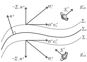
Figure 1: The spin basis vector field $\sigma^{A}$ in the neighborhood of the brane $\Sigma_{0}$. $\sigma^{A}_{\pm}$ are mirror images of one another, which is what one might expect of an ordinary vector under the $\mathbb{Z}_{2}$ symmetry. For reference, we show how an axial spin vector $S^{A}$ would transform under $\mathbb{Z}_{2}$, with its tangential components reversed.

This continuation of $\sigma^{A}$ across the brane can be viewed as a way out of our dilemma because the observationally accessible part of $\sigma^{A}$ has a well defined limiting value as $\ell\rightarrow 0$. In this case, the dynamics of $\sigma^{\alpha}$ and $\varSigma$ can be worked out using equations (70) on either the $+$ or $-$ side with the assurance that the answer for $\sigma^{\alpha}$ will be the same. Whether or not this mathematical trick has any physical relevance is an open question; the skeptical reader may conclude that the discontinuity in the geometry precludes sensible descriptions of 5D spin tensors on the brane, which could be viewed as an indictment of the thin-brane picture. At any rate, our formalism can be freely applied to smooth manifolds, which include thick-brane solutions. In the next section, we will look at a specific example of gyroscope motion from 5D non-compactified Kaluza-Klein theory.

V.4 Variation of 4D spin in a cosmological setting

We now turn our attention to a specific metric which has been used to embed standard $k=0$ Friedmann-Lemaître-Robertson-Walker (FLRW) cosmologies in a 5D flat space. The line element, which was first given by Ponce de Leon Ponce de Leon (1988), is

$$d\mathcal{S}^{2}=\ell^{2}\,dt^{2}-a^{2}(t,\ell)d\roarrow{x}\cdot d\roarrow{x}-\frac{\alpha^{2}t^{2}}{(1-\alpha)^{2}}\,d\ell^{2},$$ (79)

where $\roarrow{x}=(x,y,z)$, $\alpha$ is a parameter, and

$$a(t,\ell)=t^{1/\alpha}\ell^{1/(1-\alpha)}.$$ (80)

This metric is a solution of $R_{ABCD}=0$; i.e. it is 5D Minkowski space written in complicated coordinates. The $\ell=$ constant hypersurfaces of this metric share the same geometry as a $k=0$ FLRW solution with a scale factor equal to $a(t,\ell)$, which in turn corresponds to matter with an equation of state $p=(2\alpha/3-1)\rho$. The way in which the 4D big bang is embedded by metrics of the form (79) has been discussed in detail elsewhere Wesson and Seahra (2001); Seahra and Wesson (2002).

In this section, we will consider a pointlike gyroscope confined to move on one of the $\Sigma_{\ell}$ hypersurfaces by a non-gravitational centripetal force as discussed in Section IV. Our goal will be to solve equations (70) for the orbits of the spin basis vectors $\{\sigma^{\alpha}_{a},\varSigma_{a}\}$. We make the simplest possible choice for coordinates on $\Sigma_{\ell}$, namely $y^{\alpha}=(t,x,y,z)$ so that $e^{A}_{\alpha}=\delta^{A}_{\alpha}$. Let us introduce a set of basis vectors on $\Sigma_{\ell}$:

$$\lambda^{\alpha}_{(0)} = u^{\alpha}=[\ell^{-1}f(t,\ell),\beta a^{-2}(t,\ell),0,0],$$ (81a)

$$\lambda^{\alpha}_{(1)} = \bar{u}^{\alpha}=a^{-1}(t,\ell)[\beta\ell^{-1},f(t,\ell),0,0],$$ (81b)

$$\lambda^{\alpha}_{(2)} = \hat{y}^{\alpha}=a^{-1}(t,\ell)[0,0,1,0],$$ (81c)

$$\lambda^{\alpha}_{(3)} = \hat{z}^{\alpha}=a^{-1}(t,\ell)[0,0,0,1].$$ (81d)

Here, $\beta$ is a parameter and the function $f(t,\ell)$ is given by

$$f(t,\ell)=\sqrt{1+\beta^{2}a^{-2}(t,\ell)}.$$ (82)

It is not difficult to verify that this basis is orthonormal:

$$\eta_{(\mu)(\nu)}=h_{\alpha\beta}\lambda^{\alpha}_{(\mu)}\lambda^{\beta}_{(\nu)},$$ (83)

where $\eta_{(\mu)(\nu)}=\mathrm{diag}(1,-1,-1,-1)$. Also, one can verify that the basis is parallelly-propagated along the integral curves of $u^{\alpha}$:

$$u^{\alpha}\nabla_{\alpha}\lambda^{\beta}_{(\mu)}=0.$$ (84)

Hence, $u^{\alpha}$ is tangent to geodesics on $\Sigma_{\ell}$ and the other members of $\{\lambda^{\alpha}_{(\mu)}\}$ are 4D FW transported along those geodesics. These geodesics represent a particle moving in the $x$-direction with a proper speed of $\beta/a^{2}(t,\ell)$. As demonstrated in Section IV, when test particles are confined to a given $\Sigma_{\ell}$ hypersurface they will travel on geodesics of that hypersurface. Therefore, we can take our gyroscope to be traveling on one of the $u^{\alpha}$ integral curves. Also notice that if the spin basis were 4D FW transported along the integral curves of $u^{\alpha}$, the projections of $\sigma_{a}^{\alpha}$ onto $\{\lambda^{\alpha}_{(\mu)}\}$ basis would be constant. We shall see that this is not the case for 5D FW transport.

Having specified the form of the trajectory, we turn our attention to equations (70). By calculating the extrinsic curvature of the $\Sigma_{\ell}$ hypersurfaces and substituting in the expression (81a) for $u^{\alpha}$, we can determine the anomalous torque defined by equation (71):

$$\tau^{\alpha}=\frac{\beta\varSigma}{t\ell}\left[\frac{f(t,\ell)}{a(t,\ell)}\right]\bar{u}^{\alpha}.$$ (85)

Interestingly enough, the anomalous torque vanishes if the gyroscope is comoving with $\beta=0$. This is demanded by isotropy; a nonzero $\tau^{\alpha}$ for comoving paths would pick out a preferred spatial direction.

Continuing, we suppress the Latin index on $\sigma^{\alpha}_{a}$ and $\varSigma_{a}$. Now, equation (73) gives that $\sigma^{\alpha}$ is orthogonal to $u^{\alpha}$. We can therefore expand any spin basis vector as follows

$$\sigma^{\alpha}=\sigma\hat{\sigma}^{\alpha},\quad-1=\hat{\sigma}_{\alpha}\hat{\sigma}^{\alpha},\quad 0=u_{\alpha}\hat{\sigma}^{\alpha},$$ (86)

with

$$\hat{\sigma}^{\alpha}=\bar{u}^{\alpha}\cos\theta+\sin\theta(\hat{y}^{\alpha}\cos\phi+\hat{z}^{\alpha}\sin\phi).$$ (87)

Here, $(\sigma,\theta,\phi)$ are considered to be functions of $t$ and $\ell$ and can be thought of as the spherical polar components of $\sigma^{\alpha}$. Equation (70c) gives

$$1=\sigma^{2}+\varSigma^{2},$$ (88)

which motivates the ansatz

$$\sigma=\sin\gamma(t,\ell),\quad\varSigma=\cos\gamma(t,\ell).$$ (89)

Figure 2 depicts the decomposition of $\sigma^{A}$ in the $\{\lambda^{\alpha}_{(i)},n^{A}\}$ basis. (Recall that since $u^{A}\sigma_{A}=0$, $\sigma^{\alpha}$ will have no projection on $\lambda^{\alpha}_{(0)}=u^{\alpha}$.)

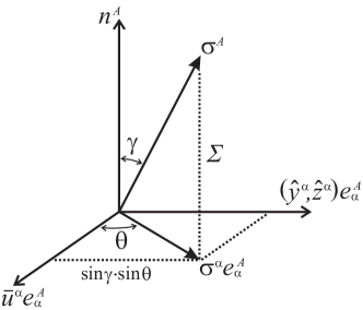
Figure 2: The decomposition of $\sigma^{A}$ in the $\{\lambda^{\alpha}_{(i)},n^{A}\}$ basis.

Substituting equations (85) – (89) into equation (70a) and taking scalar products with each of $\{\lambda^{\alpha}_{(\mu)}\}$ basis vectors yields an integrable set of first order differential equations for $(\gamma,\theta,\phi)$. We omit the details and quote the results:

$$\cos\gamma = \cos\varphi_{1}\cos[\varphi_{2}+\alpha\beta a^{-1}(t,\ell)],$$ (90a)

$$\sin\varphi_{1} = \sin\gamma\sin\theta,$$ (90b)

$$\phi = \varphi_{3},$$ (90c)

where we require

$$-\tfrac{\pi}{2}\leq\varphi_{1}\leq\tfrac{\pi}{2},\quad\sin\gamma\neq 0.$$ (91)

Here, the angles $\{\varphi_{i}\}$ are constants of integration. Equation (90a) governs the evolution of $\sigma^{\alpha}\sigma_{\alpha}$ and $\varSigma$, while equations (90b) and (90c) state that the projection of $\sigma^{\alpha}$ onto the plane spanned by $\hat{y}^{\alpha}$ and $\hat{z}^{\alpha}$ is of constant magnitude. In the late epoch limit we have that $a(t,\ell)\rightarrow\infty$, which implies that $\cos\gamma$ and $\sin\theta$ approach constant values. In other words, the spin basis vectors become static for late times. As mentioned above, they are also static for comoving gyros with $\beta=0$. For early times, the variation of the $\gamma$ and $\theta$ angles implies that the spin basis vector precess with respect to a 4D non-rotating frame.

To make contact with 4D physics, we must now specify a set of four linearly independent spin basis vectors by choosing four different sets of the constant angles $\{\varphi_{i}\}$. We can then construct a 4D spin tensor from equation (74), with $\sigma^{ab}$ arbitrary. We will not do that explicitly here, we rather content ourselves with the observation that equations (74), (76), (89) and (90a) imply that the magnitude of the 4D spin $\sigma^{\alpha\beta}\sigma_{\alpha\beta}$ is not conserved. In fact, it is not difficult to show that in the $a\rightarrow\infty$ limit the derivative of the spin magnitude obeys

$$\left|\frac{d}{da}\sigma^{\alpha\beta}\sigma_{\alpha\beta}\right|\propto a^{-2}.$$ (92)

Because this variation takes place on cosmic timescales, it is not likely to be observed by an experiment like Gravity Probe B. However, the example in this section was intended to be illustrative of the method rather than an experimental suggestion. Application of the formalism to other higher dimensional scenarios may lead to experimentally or observationally testable effects. We hope to report on such matters in the future.

VI Summary and Conclusions

In this paper, we have used the $(3+1)+1$ dimensional foliation of a non-compact 5D manifold described in Section II to analyze various aspects of test particle and pointlike gyroscope motion in higher dimensions.

In Section III.1, we split the 5D affinely-parameterized geodesic equation into a 4D equation of motion (26a), an equation governing the motion perpendicular to $\Sigma_{\ell}$ (26b), and an equation describing the evolution of the norm of the 4-velocity (26c). We also demonstrated that these three equations were not independent. In Section III.2, we described how equations (26) behave under a general change of parameter (equations 32). We then gave their form in the 4D proper time parameterization (equations 35 and 38). In the latter case, we saw that the 4-velocity was properly orthogonal to the 4-acceleration. In Section III.3, we showed that the projected 4-velocity $u^{\alpha}=e^{\alpha}_{A}u^{A}$ does not equal $dy^{\alpha}/d\lambda$, but rather corresponds to the velocity in canonical coordinates. We also saw that the fifth force $f^{\alpha}$ defined by equation (41) is not equal to the 4-acceleration and does not transform as a 4-vector under $y^{\alpha}\rightarrow\tilde{y}^{\alpha}(y^{\beta})$.

In Section IV, we derived the form of the force required to confine a particle to a single $\Sigma_{\ell}$ hypersurface and showed that it reduced to the ordinary centripetal force in Minkowski space. We also demonstrated that particles travel on geodesics of $\Sigma_{\ell}$ under these conditions.

In Section V.1, we showed how the problem of determining the 5D orbit of a pointlike gyroscope can be reduced to the solution of the Fermi-Walker transport equation, just as in 4D, but relation to the spin tensor is different than in the spacetime case. In Section V.2, we performed a $(3+1)+1$ split of the 5D FW equation for the case of freely falling gyroscopes (equation 66) and confined gyroscopes (equation 70). We demonstrated that in both cases, the magnitude of the 4D spin is not conserved due to the existence of an anomalous torque. In Section V.3, we discussed how our results should be interpreted in the thin brane world scenario. In Section V.4, we applied our formulae to a specific 5D cosmological example and derived how the 4D spin of a gyroscope varies when confined to a $\Sigma_{\ell}$ hypersurface.

In conclusion, we mention a few possible directions for future work. Equations (26) can be used to study the motion of observers in the thick brane world and non-compact Kaluza-Klein theories, apparent violations of 4D causality due to the existence of 5D “short-cuts”, and the effect of 5D dynamics on astrophysical systems. Equation (26b) can be used to study the issue of whether a given 3-brane attracts or repels test particles. On the theoretical side, an interesting exercise involves determining how the extra acceleration $a^{\alpha}(u)$ encodes the electromagnetic force previously observed in the fifth force $f^{\alpha}(u)$ derived from the 5D geodesic equation. The discrepancy between the 5D affine parameter and the 4D proper time seen in Section III.2 raises the question of which one is the correct “clock” to use, which certainly merits close attention. Our formalism concerning pointlike gyroscopes should be applied to 5D static and spherically-symmetric metrics in order to make predictions testable by Gravity Probe B. The issue of the cosmological variation of spin can be applied to the evolution of the angular momentum of galaxies, pulsars and high-energy primordial objects. These ideas do not comprise an exhaustive list of potential avenues of exploration, which underlines the generality and wide applicability of formulae derived in this paper.