Circular orbits of corotating binary black holes: comparison between analytical and numerical results

Abstract

We compare recent numerical results, obtained within a“helical Killing vector” (HKV) approach, on circular orbits of corotating binary black holes to the analytical predictions made by the effective one body (EOB) method (which has been recently extended to the case of spinning bodies). On the scale of the differences between the results obtained by different numerical methods, we find good agreement between numerical data and analytical predictions for several invariant functions describing the dynamical properties of circular orbits. This agreement is robust against the post-Newtonian accuracy used for the analytical estimates, as well as under choices of resummation method for the EOB “effective potential”, and gets better as one uses a higher post-Newtonian accuracy. These findings open the way to a significant “merging” of analytical and numerical methods, i.e. to matching an EOB-based analytical description of the (early and late) inspiral, up to the beginning of the plunge, to a numerical description of the plunge and merger. We illustrate also the “flexibility” of the EOB approach, i.e. the possibility of determining some “best fit” values for the analytical parameters by comparison with numerical data.

I Introduction

Binary black holes are the most promising candidate sources for the LIGO / VIRGO / GEO600 / TAMA $\ldots$ network of ground based gravitational wave (GW) interferometric detectors LPP97 ; FH98 ; BCT98 ; PZM ; DIS00 . Signal to noise ratio estimates suggest that the first detections will concern black hole binaries of total mass $\gtrsim 25\,M_{\odot}$, and show that the most “useful” part of the gravitational waveform is emitted in the last $\sim 5$ orbits of the inspiral, and during the plunge taking place after crossing the last stable (circular) orbit (LSO) DIS00 . This makes it urgent to have reliable methods allowing one to model the last orbits of binary black holes.

Recently, Ref. BD00 has suggested a new method to tackle the dynamics and GW emission from the last orbits of binary black holes. The basic idea of BD00 was to extend, by using suitable resummation methods, the validity of the perturbative (“post-Newtonian”) analytical calculations of the equations of motion DD ; JS98 ; DJS01 ; BF00 and GW radiation BDIWW ; B so as to be able to describe not only the last orbits before the LSO, but also the transition to the plunge. The main philosophy of BD00 was to push analytical methods to their limits so as to use numerical methods only to describe the plunge, which was estimated (when the masses are comparable) to last about 60% of one orbit. To implement this philosophy, one needs to be able to construct numerical initial data that match the dynamical initial data given by the method of BD00 at the start of the plunge. This is a non trivial task because, up to very recently, there was a significant discrepancy between analytical DIS98 ; BD00 ; DJS00 ; B02 and numerical cook ; PfeifTC00 ; baumgarte estimates of the dynamical characteristics of the orbits near the LSO. For instance, the binding energy at the LSO, $e_{\rm LSO}=E_{\rm LSO}/(m_{1}+m_{2})-1$, is analytically estimated to be around $e_{\rm LSO}^{\rm ana}\simeq-1.67$% DJS00 (third post-Newtonian effective-one-body estimate with $\omega_{s}=0$ DJS01 ), while two different numerical estimates cook ; baumgarte gave $e_{\rm LSO}^{\rm num}\simeq-2.3$%, i.e. a significantly more bound (by 38%) LSO. The discrepancy is even more striking if one considers the LSO orbital period: the analytical estimate is $T_{\rm LSO}^{\rm ana}\simeq 71.2\,(m_{1}+m_{2})$ DJS00 , which is twice longer than the numerical one $T_{\rm LSO}^{\rm num}\simeq 35\,(m_{1}+m_{2})$ baumgarte . [By contrast, the dispersion among analytical estimates DIS98 ; BD00 ; DJS00 ; B02 , as well as the dispersion among numerical ones cook ; PfeifTC00 ; baumgarte is significantly smaller than the difference between analytical and numerical results. See Buona02 for a review of analytical methods, and see below for a brief discussion of our choice of analytical estimates.] This discrepancy diminishes the physical relevance of a recent attempt baker at fulfilling the proposal of Ref. BD00 , i.e. to start a full numerical calculation of the plunge just after the crossing of the LSO.

Very recently, a new numerical approach to the circular orbits of binary black holes has been set up GGB1 and implemented GGB2 (see also Ref. Cook02 for a discussion and an extension to any black hole rotation state). Contrary to the previous numerical approaches cook ; PfeifTC00 ; baumgarte , which were formulated in terms of the initial value problem of general relativity and dealt therefore only with the four constraint equations on a 3-dimensional spacelike hypersurface, the new approach GGB1 deals with a full 4-dimensional spacetime (see Ref. Cook02 for the link with York’s conformal thin-sandwich formalism York99 ; Cook00 ). The basic assumption is that this spacetime is endowed with a helical Killing vector Detwe89 , which amounts to neglecting the gravitational radiation reaction, i.e. to considering that the orbits are exactly circular. In addition, Refs. GGB1 ; GGB2 assume, as a simplifying approximation, that the spatial 3-metric is conformally flat (see Sec. IV.C of Ref. FriedUS02 for a discussion). The slicing is also chosen to be maximal (i.e. $K=0$). The spacetime manifold is chosen to have the topology of the real line times the two-sheeted Misner-Lindquist manifold. The two sheets are assumed to be isometric (with respect to the full 4-metric). Under the above assumptions, the problem amounts to solving five of the ten Einstein equations. This is one more that the previous numerical approaches cook ; PfeifTC00 ; baumgarte . Hereafter we call the new method GGB1 ; GGB2 the helical Killing vector (HKV) approach, and previous methods cook ; PfeifTC00 ; baumgarte IVP ones (for Initial Value Problem). Note that the HKV approach has also been employed for binary neutron stars (see e.g. GourgGTMB01 and references therein).

The first numerical results obtained by the HKV method GGB2 for the characteristics of the LSO indicate a much better agreement with analytical estimates than those obtained with the IVP method cook ; PfeifTC00 ; baumgarte . However, the comparison, done in GGB2 , used analytical results valid only for non spinning black holes, while the numerical approach of GGB1 concerns corotating binary black holes. Moreover, the comparison made in GGB2 was limited to the sole LSO, without looking at the behavior of the other circular orbits. It is known that the presence of even small additional interactions (especially repulsive ones) can have an important effect on the dynamical characteristics of the orbits around the LSO. It is therefore a priori necessary to include spin-orbit effects (which are repulsive in the corotating case) when doing the analytical/numerical comparison. Fortunately, a recent analytical work D01 has shown how to generalize the effective one body (EOB) approach of BD00 by including, to lowest order, spin-orbit and spin-spin effects. The purpose of the present work is to take into account in detail the effect of the spin interactions in corotating binary black holes. Another important feature of this work is that we shall compare the predictions of the EOB method BD00 ; DJS00 ; D01 and the results of the new numerical approach of GGB1 ; GGB2 , not only for the characteristics of the LSO (to which most authors limit their considerations), but also for all other circular orbits. We shall do that by comparing several physically important (and coordinate-invariant) functions, such as the binding energy as a function of angular velocity. Note that, in this work, we loosely call “LSO”, for a corotating system, the maximal binding configuration along a corotating sequence. For HKV sequences, it has been shown that this minimal energy configuration marks the onset of an orbital instability FriedUS02 . The fact that such corotating sequences are (probably) not realized in actual coalescing systems, and that the corotating “LSO” signals only a secular instability, is not important for the present work whose main aim is to show how one can relate the numerical and analytical descriptions of the same configuration involving spinning black holes.

This paper is organized as follows. Section II discusses the arguments selecting the EOB method as the current best analytical method for tackling the last orbits of binary black holes and summarizes the EOB approach to spinning black holes. Section III applies the EOB formalism to corotating black holes on circular orbits and shows how to compare the analytical results to the recent numerical computation of a sequence of corotating binary black holes. Section IV discusses the meaning of our results.

II Effective one-body approach to spinning binary black holes

II.1 Formulation

Before summarizing the effective one-body (EOB) formalism, let us recall why we consider it as the best current analytical formalism for tackling the dynamics of the last orbits of binary black holes. The first point is that the second work in Ref. DIS00 has shown that it is crucial, if one wishes to keep a good overlap with the expected real signals, to generate GW templates which go beyond the “adiabatic approximation” and which use accurate equations of motion, including radiation reaction, to describe the smooth transition (taking place around the LSO) between inspiral motion and plunge. However, the most accurate equations of motion DD ; JS98 ; DJS01 ; BF00 are a priori given as very complicated expressions, containing hundreds of terms. These equations of motion are essentially power series in a formal “small parameter” $\epsilon\sim GM/c^{2}r\sim v^{2}/c^{2}$ [“post-Newtonian” (PN) expansion]. The problem is that the “small” PN expansion parameter $\epsilon$ is not numerically very small near the LSO. It was found quite early that the use of straightforward PN-expanded equations of motion (as in LW90 ) is unsatisfactory because the PN-expanded equations of motion converge so slowly that, at low orders, they can lead to a behavior which is qualitatively different from what one expects. In particular, it was shown in KWW93 that the PN-expanded (harmonic-coordinates) equations of motion admit an LSO at the second post-Newtonian (2PN) level, but admit no LSO at both the first post-Newtonian (1PN) and the third post-Newtonian (3PN) levels. [ “LSO” is taken here in the sense of a critical point in the dynamical analysis of circular orbits.] By contrast, a study of the LSO in terms of the PN-expanded Hamiltonian WS has found that the PN-expanded Hamiltonian (in various coordinates) admits no LSO at the 2PN level, but admit LSO’s at the 1PN and 3PN levels. This unstable behavior is a sign of the unreliability of non-resummed PN approaches.

As the recent work JS98 ; DJS01 ; BF00 has succeeded in deriving complete 3PN equations of motion, it would be unacceptable to “spoil” the precious information they contain by using them in such an inappropriate way. This led Ref. KWW93 to propose to improve the situation by using a partial resummation approach. Specifically, they introduced an “hybrid” approach in which one resums exactly the “Schwarzschild” terms in the (relative) equations of motion, while continuing to treat the $\nu$-dependent terms (where $\nu\equiv m_{1}\,m_{2}/(m_{1}+m_{2})^{2}$) as straightforward PN expansions. This “hybrid” approach did improve the situation to some extent (at least at the 2PN accuracy). However, later work showed that the hybrid approach was neither robust, nor consistent. Ref. WS showed that the predictions of the hybrid approach were robust neither under using Hamiltonian equations of motion instead of Newtonian-like ones, nor under a change of coordinate system. Ref. DIS98 pointed out the inconsistency of the hybrid method by showing that the formal (un-resummed) “$\nu$-corrections” represent, in several cases, a very large (larger than 100%) modification of the corresponding resummed $\nu$-independent terms. This led to a quest for new resummation approaches providing full dynamical equations of motion for binary systems, and being robust and consistent. The only such method we are aware of is the EOB approach BD00 . We do not consider here methods such as the $E$- or $e$-methods of DIS98 and the $j$-method of DJS00 which were devised to investigate the location of the LSO. These methods cannot be used beyond the “adiabatic approximation” because they do not provide full dynamical equations of motion able to model the transition between inspiral and plunge. Let us note in this respect that the work of BD00 has shown that, in the case of comparable masses, the transition between inspiral and plunge is a gradual process in which the precise location of the “adiabatic” LSO is less important than a precise evaluation of radiation damping effects. Therefore it is finally not very important to focus on the “exact” location of the LSO. What is really important is to have a good description of the dynamics of the last ten orbits before the plunge. Moreover, even if we were to consider only the determination of the LSO, the comparisons made in DJS00 have shown that the EOB method is the most robust in that it is the least sensitive to changes in the 3PN coefficients (see Fig. 2 in DJS00 ). We also note in passing that DIS98 had shown that the $e$-method was more robust (both in its dependence on $\nu$ and under changes in higher PN coefficients), and more convergent, than the straightforward non resummed $E$-method (recently used at 3PN in B02 ); see Table I, Table VII and Fig. 5 in DIS98 . The robustness of the EOB method is discussed in Refs. BD00 ; DJS00 ; D01 . We shall give below further examples of the robustness of the EOB approach.

The basic idea of the EOB method is to map the (complicated) relative dynamics (in the center of mass) of a two-body system onto the (drastically simpler) dynamics of an “effective” one-body system. Most of the (physically irrelevant) gauge-related complications of the two-body equations of motion get absorbed into the mapping between the two problems. The mapping is defined so as to preserve the adiabatic invariants (which, at the quantum level, are quantized in units of $\hbar$). The energy mapping $E_{\rm eff}=f(E_{\rm real})$ between the real two-body (center of mass) energy $E_{\rm real}$ and the effective one-body energy $E_{\rm eff}$ is determined by the matching between the two problems. It is remarkably found that the energy map $f$ is extremely simple, and independent of the PN accuracy considered (we set $c=1$):

$$\frac{E_{\rm eff}}{\mu}=\frac{E_{\rm real}^{2}-m_{1}^{2}-m_{2}^{2}}{2\,m_{1}\,m_{2}}\,.$$ (1)

Here, $m_{1}$ and $m_{2}$ denote the masses of the two bodies, while $\mu$ denotes the reduced mass $\mu=m_{1}\,m_{2}/M$, with $M=m_{1}+m_{2}$ denoting the total mass. Let us note also the definition of the symmetric mass ratio $\nu\equiv\mu/M=m_{1}\,m_{2}/(m_{1}+m_{2})^{2}$ ($0<\nu\leq\frac{1}{4}$). The inverse of the energy map (1) is

$$E_{\rm real}=M\,\sqrt{1+2\nu\left(\frac{E_{\rm eff}-\mu}{\mu}\right)}\,.$$ (2)

The effective energy $E_{\rm eff}$ is given by the effective Hamiltonian $H_{\rm eff}(\mbox{\boldmath$x$},\mbox{\boldmath$p$},\mbox{\boldmath$S$}_{1},\mbox{\boldmath$S$}_{2})$. Here, $x$ and $p$ are the positions and momenta of the effective one-body (describing the relative motion) and $\mbox{\boldmath$S$}_{1}$ and $\mbox{\boldmath$S$}_{2}$ are the two independent spin vectors of the two bodies. Ref. BD00 considered only the 2PN approximation and the spin-independent case. The 3PN, spin-independent effective Hamiltonian was determined in DJS00 . Ref. D01 recently showed how to add the spin interactions in the EOB framework. The most complete version of the 3PN spin-dependent effective Hamiltonian is given by Eq. (2.56) of D01 . For simplicity, and because spin-spin effects will turn out to be quite small, we shall consider the less complete, but simpler, effective Hamiltonian defined by Eq. (2.26) of D01 with the effective metric defined by the “deformed Kerr metric” of Section IIC there. This Hamiltonian takes into account (at the lowest PN approximation) the full spin-orbit interaction, and incorporates most of the spin-spin interaction. [In the case of parallel spins the ratio between the spin-spin interaction included in the simplified $H_{\rm eff}$ and the more complete one $H^{\prime}_{\rm eff}$ is $\left(\frac{7}{8}\right)^{2}$.] The Kerr parameter of the effective Kerr metric describing spin-orbit and spin-spin interactions is given by

$$M\mbox{\boldmath$a$}\equiv\mbox{\boldmath$S$}_{\rm eff}\equiv\sigma_{1}\,\mbox{\boldmath$S$}_{1}+\sigma_{2}\,\mbox{\boldmath$S$}_{2}\,,$$ (3)

where $\sigma_{1}\equiv 1+3\,m_{2}/(4\,m_{1})$, $\sigma_{2}\equiv 1+3\,m_{1}/(4\,m_{2})$.

The EOB approach can deal with the most general case where the spin vectors $\mbox{\boldmath$S$}_{1}$, $\mbox{\boldmath$S$}_{2}$ are arbitrarily oriented. In fact, one of the great advantages of the EOB approach is that, being Hamiltonian-based, it provides a full set of evolution equations for all the dynamical variables: $x$, $p$, $\mbox{\boldmath$S$}_{1}$ and $\mbox{\boldmath$S$}_{2}$. See Eqs. (3.1)–(3.4) of D01 . Here, we are interested in comparing the EOB predictions with the numerical results of GGB1 ; GGB2 which are restricted to the simple case where $\mbox{\boldmath$S$}_{1}$ and $\mbox{\boldmath$S$}_{2}$ are aligned with the orbital angular momentum $L$. In this case, it was shown in D01 that, for a given effective energy $E_{\rm eff}$, and a given angular momentum $L$, the (effective) radius $r=|\mbox{\boldmath$x$}|$ of the circular orbits is obtained by solving the two equations, $R(r,E_{\rm eff},L)=\frac{\partial}{\partial r}\,R(r,E_{\rm eff},L)=0$, where $R$ is a certain effective radial potential. [We use the fact that the Carter-like constant ${\cal Q}$ vanishes for the “equatorial” orbits that we are considering.] Actually, it is more convenient to work with the inverse radial variable $u\equiv M/r$ (we set $G=1$) and with the corresponding $u$-potential $U(u)=\mu^{-2}\,r^{-4}\,R(r)$. Let us also introduce the following dimensionless variables (note that $L\equiv L_{z}$ for the orbits we consider and that, by definition, $L=L_{\rm eff}=L_{\rm real}$)

$$\widehat{E}\equiv\frac{E_{\rm real}}{\mu}\ ,\quad\widehat{L}\equiv\frac{L}{\mu M}\ ,\quad\widehat{a}\equiv\frac{a}{M}\,,$$ (4)

and

$$\overline{E}\equiv\frac{E_{\rm eff}}{\mu}\ ,\quad\overline{L}\equiv\frac{L-a\,E_{\rm eff}}{\mu M}\equiv\widehat{L}-\widehat{a}\,\overline{E}\,.$$ (5)

The quantity $a$ entering these equations is the modulus of the effective Kerr parameter defined by Eq. (3).

In terms of these quantities the (scaled) $u$-potential reads

$$U(u)=(\overline{E}-\widehat{a}\,\overline{L}\,u^{2})^{2}-\overline{A}(u)\,(1+\overline{L}^{2}\,u^{2})\,,$$ (6)

where the function $\overline{A}(u)\equiv A(u)+\widehat{a}^{2}\,u^{2}$ will be discussed below.

The sequence of circular orbits is defined by the solutions of the two equations

$$U(u,\overline{E},\overline{L})=0=\frac{\partial}{\partial u}\,U(u,\overline{E},\overline{L})\,.$$ (7)

The effective Hamiltonian $\overline{E}=\overline{H}_{\rm eff}(u,\widehat{L})$ would be obtained by solving $U(u,\overline{E},\widehat{L}-\widehat{a}\,\overline{E})=0$ which is a quadratic equation in $\overline{E}$. However, the intrinsic simplicity of the EOB approach is more visible if we use the variable $\overline{L}\equiv\widehat{L}-\widehat{a}\,\overline{E}$ instead of $\widehat{L}\equiv L/\mu M$. Indeed, the solution of $U(u,\overline{E},\overline{L})=0$ reads

$$\overline{E}=\widehat{a}\,\overline{L}\,u^{2}+\sqrt{\overline{A}(u)(1+\overline{L}^{2}\,u^{2})}\,.$$ (8)

This result can be viewed as a simple modification by spin-orbit $(\widehat{a}\,\overline{L}\,u^{2}$ term) and spin-spin effects $(\widehat{a}^{2}\,u^{2}$ contribution to $\overline{A}(u)=A(u)+\widehat{a}^{2}\,u^{2}$) of the radial potential for circular orbits in a spherically symmetric gravitational potential (such as a Schwarzschild metric, or the effective metric in absence of spins): $\overline{E}_{0}(u,\widehat{L})=\sqrt{A(u)(1+\widehat{L}^{2}\,u^{2})}$. In such a situation $A(u)$ would simply be (minus) the time-time component of the (effective) metric ($1-2u$ in the Schwarzschild case). A nice feature of the EOB approach is that, in the spin-independent case, the dynamics of circular orbits is fully encoded in only one function: the function $A(u)=-g_{00}^{\rm eff}(u)$, with $u=M/r$. [As discussed in BD00 ; DJS00 ; D01 , the dynamics of non circular orbits involves two more functions: $D(u)$ and $Q_{4}(u,p)$.] It is truly remarkable that the hundreds of complicated contributions entering the PN-expanded two-body equations of motion get drastically compactified in so few functions. In particular, for circular orbits, the essential physical information of the PN-expanded dynamics is contained in the effective metric coefficient

$$A(u)=1-2u+2\nu\,u^{3}+a_{4}(\nu)\,u^{4}+{\cal O}(u^{5})\,.$$ (9)

Note that there are no 1PN ($\propto u^{2}$) contribution in $A(u)$, and that the 2PN effects amount to the very simple term $+\,2\nu\,u^{3}$ BD00 . The 3PN contribution $\propto u^{4}$ was found DJS00 to have the coefficient

$$a_{4}(\nu)=\left(\frac{94}{3}-\frac{41}{32}\,\pi^{2}+2\,\omega_{s}\right)\,\nu\,.$$ (10)

Again, remarkable simplifications happened in the calculation of the 3PN effective metric. The 3PN coefficient $a_{4}(\nu)$ could, a priori, have involved contributions proportional to $\nu^{2}$ and $\nu^{3}$. All such contributions canceled to leave a simple final result $a_{4}(\nu)\propto\nu$. The parameter $\omega_{s}$ entering Eq. (10) (which had been left ambiguous by the first 3PN calculations) has been recently determined to be simply $\omega_{s}=0$ DJS01 . This yields a numerical value for the general relativistic prediction for the 3PN coefficient equal to:

$$a_{4}^{\rm GR}(\nu)\simeq 18.688\,\nu\simeq 4.672\,(4\nu)\,.$$ (11)

II.2 Representation of the basic EOB function $A(u)$

The EOB method a priori determines (from the original, fully PN-expanded dynamics) only the PN-expansion of the basic function $A(u)$, or of the combination

$$\overline{A}(u)\equiv A(u)+\widehat{a}^{2}\,u^{2}=1-2\,u+\widehat{a}^{2}\,u^{2}+2\nu\,u^{3}+a_{4}(\nu)\,u^{4}+{\cal O}(u^{5})\,,$$ (12)

entering the effective radial potential (6).

In this respect let us emphasize the various senses in which the EOB approach is a “resummation” of the original, fully PN-expanded equations of motion. A first, crucial “resummation” feature of the EOB approach is the mapping of the original dynamical variables $\mbox{\boldmath$q$}_{1}$, $\mbox{\boldmath$p$}_{1}$, $\mbox{\boldmath$q$}_{2}$, $\mbox{\boldmath$p$}_{2}$ onto the effective variables $x$, $p$. This mapping BD00 ; DJS00 is given as a complicated PN expansion, and provides a first level of simplification and compactification of the dynamics. A second feature consists in the fact that the real Hamiltonian is given by an iterated square-root. For instance, in the spin-independent case ($\widehat{\mbox{\boldmath$p$}}\equiv\mbox{\boldmath$p$}/\mu$)

$$H_{\rm real}(\mbox{\boldmath$x$},\widehat{\mbox{\boldmath$p$}})=M\sqrt{1+2\nu\left(-1+\sqrt{A(r)\left(1+\widehat{\mbox{\boldmath$p$}}^{2}+\left(\frac{A(r)}{D(r)}-1\right)(\mbox{\boldmath$n$}\cdot\widehat{\mbox{\boldmath$p$}})^{2}+\widehat{Q}_{4}(\widehat{\mbox{\boldmath$p$}})\right)}\right)}\,.$$ (13)

This iterated square-root structure is, by itself, a partial resummation because the fully PN-expanded Hamiltonian, which has the form $H_{\rm real}(\widehat{p})=$ $M[1+\nu\left(\frac{1}{2}\,\widehat{\mbox{\boldmath$p$}}^{2}+\frac{M}{r}\right)+\cdots+$ $c_{8}\,\widehat{\mbox{\boldmath$p$}}^{8}+\cdots+{\cal O}(\widehat{\mbox{\boldmath$p$}}^{10})]$, would be obtained by re-expanding all this square-root structure in powers of $\widehat{\mbox{\boldmath$p$}}^{2}$ and $M/r$. Finally, on top of these two partial resummations, it is very natural, within the EOB approach, to further resum $H_{\rm real}$ by replacing the PN-expanded results for $A(u)$, Eq. (9), and/or $\overline{A}(u)$, Eq. (12), by some better behaved expressions. Indeed, as we recalled above, in the spin-independent case $A(u)$ plays the basic role of replacing $-\,g_{00}^{\rm Schwarz}=1-2M/r$ in the radial potential determining the circular orbits.

It is then natural to require that the “exact” effective $A(u)$ should have the same qualitative behavior as $1-2u$, i.e. a simple zero at a finite value of $u$. More generally, in the spin-dependent case $\overline{A}(u)$ is a $\nu$-deformation of the Kerr function $r^{-2}\,\Delta_{t}(r)=r^{-2}(r^{2}-2\,Mr+a^{2})$ which determines the location of the horizon. It is therefore natural to require that the effective $\overline{A}(u)$ have, like $1-2u+\widehat{a}^{2}\,u^{2}$, a simple zero at a finite value of $u$. To ensure such a qualitative behavior it is natural to replace the straightforward Taylor expansion giving $\overline{A}(u)$ by a suitable Padé approximant (chosen so as to robustly imply the presence of a simple zero), namely D01

$$\overline{A}(u,\widehat{a}^{2})=P_{3}^{1}\,[1-2u+\widehat{a}^{2}\,u^{2}+2\nu\,u^{3}+a_{4}(\nu)\,u^{4}]\,,$$ (14)

where $P_{m}^{n}$ denotes a Padé of the $N_{n}/D_{m}$ type (where the indices denote the degrees of the numerator and denominator).

As a test of the robustness of the EOB predictions we shall also consider a more brutal way of ensuring that $A(u)$ has a simple zero at a finite value of $u$: it consists in defining

$$\overline{A}^{\prime}(u,\widehat{a}^{2})=(1-2u)(1+2\nu\,u^{3}+(a_{4}(\nu)+4\nu)\,u^{4})+\widehat{a}^{2}\,u^{2}\,.$$ (15)

Fig. 1 compares the various representations of the function $\overline{A}(u)$: the straightforward Taylor series approximant (12) (truncated after the 3PN term $\propto u^{4}$), the Padé approximant (14) and the “factorized Taylor” approximant (15). They are represented both in the limit $\widehat{a}=0$, and for the value $\widehat{a}=0.15$ which roughly corresponds to the value of $\widehat{a}$, at the LSO, in the effective one-body formalism discussed in the next Section. Note that the various representations start differing significantly from each other only for $u\simeq 0.4$, i.e. for values about twice larger than the value of $u$ corresponding to the LSO, i.e. $u_{\rm LSO}\simeq 0.22$. However, this does not mean that the resuming of $\overline{A}(u)$ and/or the addition of the spin-dependent interactions has no significant effect on the characteristics of the LSO. Indeed, as the usual (non corotating) LSO corresponds to an inflection point in the effective radial potential $H_{\rm eff}(r,L,S_{a})$, any modification of the radial dependence of the Hamiltonian (e.g. by a change in $\overline{A}(u)$ or the addition of the linear spin-orbit term $\widehat{a}\,\overline{L}\,u^{2}$ in Eq. (8)) has a strong effect on the location of the LSO.

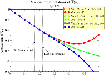
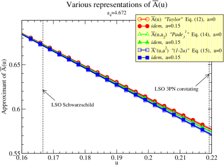
Figure 1: Various representations of the function $\overline{A}(u,\widehat{a}^{2})$. The right figure is a enlargement of the LSO region.

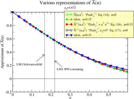
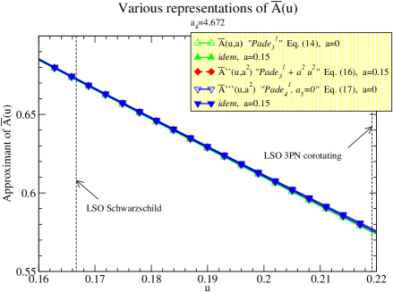
Figure 2: Various Padé approximants of the function $\overline{A}(u,\widehat{a}^{2})$. The right figure is a enlargement of the LSO region.

On the other hand, Fig. 2 compares different variants of the Padé approximants that one could use. In the text, we have followed Ref. D01 in focusing on the specific definition (14) of the function $\overline{A}(u)$. However, one could have considered

$$\overline{A}^{\prime\prime}(u,\widehat{a}^{2})=P_{3}^{1}[1-2u+2\nu\,u^{3}+a_{4}(\nu)\,u^{4}]+\widehat{a}^{2}\,u^{2}\,.$$ (16)

Another possibility arises when one uses the great “flexibility” of the EOB approach. As discussed in BD00 ; D01 one can think of the EOB formalism as a multi-parameter analytical formalism, where only a fraction of the parameters is currently known. For instance, there are further terms in the expansions (9) and (12), say $+\,a_{5}(\nu)\,u^{5}+a_{6}(\nu)\,u^{6}+\cdots$. The parameters $a_{5}(\nu),a_{6}(\nu),\ldots$ are not known at present. However, they can be introduced as fitting parameters and adjusted so as to reproduce other information one has about the exact results. For instance, if we had reason to trust some numerical results, one could search for the optimal values of $a_{4}(\nu),a_{5}(\nu),\ldots$ that best fit the numerical data. We shall give an example of this below. A minimal requirement is to test the “robustness” of the EOB formalism under adding some reasonable values for $a_{5}(\nu),\ldots$. See Ref. DIJS for a study of this robustness. Here, we just wish to illustrate a minimal aspect of this robustness: when adding the next term $a_{5}(\nu)\,u^{5}$ to $A(u)$, the natural Padé approximant to use becomes

$$\overline{A}^{\prime\prime\prime}(u,\widehat{a}^{2})=P_{4}^{1}[1-2u+\widehat{a}^{2}\,u^{2}+2\nu\,u^{3}+a_{4}(\nu)\,u^{4}+a_{5}(\nu)\,u^{5}]\,.$$ (17)

If we take the $a_{5}\rightarrow 0$ limit of the Padé approximant (17) we do not recover (14). Indeed, the $P_{3}^{1}$ approximant (14) is uniquely defined by the requirement of being $\propto N_{1}/D_{3}$ and of matching (12) up to $a_{4}\,u^{4}$. This means that $P_{3}^{1}$ effectively makes an “educated guess” about an infinite number of additional contributions $a_{5}\,u^{5}+a_{6}\,u^{6}+\cdots$, which are plausible continuations of the known terms $1-2u+\cdots+a_{4}\,u^{4}$. In particular, the Taylor expansion of $P_{3}^{1}$ must contain a non-zero contribution $a_{5}\,u^{5}$. This explains why it does not agree with the $a_{5}=0$ limit of (17). It is therefore interesting to compare (17) to (14) to measure the robustness of Padé approximants against knowledge or lack of knowledge of $a_{5}$. In fact, Fig. 2 shows that the various ways we have just described of defining some Padé approximants of $\overline{A}(u)$ give extremely close results. Much closer than the variants represented in Fig. 1. This is an illustration of the generic robustness of Padé resummation.

III Comparing analytical and numerical results for corotating binary black holes

III.1 Corotating configurations in the EOB framework

Let us now tackle the central problems of this paper: (i) to compute the coordinate-invariant functions characterizing the dynamics of adiabatic sequences of corotating binary black holes on circular orbits, and (ii) to compare the (EOB) analytical predictions with the numerical results of Refs. GGB1 ; GGB2 . The main subtlety in this study comes from the corotation assumption. This assumption means that the spins of the black holes vary along the sequence, and in fact increase as the radial distance $r$ decreases. However, any point in the sequence, i.e. any circular orbit, must be determined (in the EOB approach) by imposing that

$$0=\dot{r}=\frac{\partial H_{\rm real}(r,p_{r},L,S_{1},S_{2})}{\partial r}\,,$$ (18)

$$0=\dot{p}_{r}=-\frac{\partial H_{\rm real}(r,p_{r},L,S_{1},S_{2})}{\partial p_{r}}\,,$$ (19)

and $p_{r}=0$, where the derivatives are all considered for fixed values of $L$, $S_{1}$ and $S_{2}$. Eq. (19) is automatically satisfied by $p_{r}=0$, and Eq. (18) (with $p_{r}=0$) then leads to Eqs. (7) above. Eq. (18) determines $r$ as a function of $L$, $S_{1}$ and $S_{2}$, or $L$ as a function of $r$, $S_{1}$ and $S_{2}$. It then remains to determine how $S_{1}$ and $S_{2}$ vary as functions of $L$ and $r$. Let us also note beforehand that, in view of Eq. (18), the usual (irrotational) LSO corresponds to an inflection point (in $r$) of $H_{\rm real}(r,L,S_{a})$ considered for fixed values of $L$ and $S_{a}$ (corresponding to the LSO), and to a minimum of $H_{\rm real}$ (i.e. a maximum binding configuration) along a sequence of fixed values of $S_{a}$. In the corotating case, we define the LSO as the maximum binding configuration along a corotating sequence. The variation of $S_{a}$ with $r$ along a corotating sequence changes the location of the minimum of $H_{\rm real}$ with respect to the irrotational case. The variation of $S_{a}$ with $r$ prevents this minimum to correspond to an inflection point of the function $H_{\rm real}(r,L,S_{a})$ considered for the fixed LSO values of $L$ and $S_{a}$.

The variation of the magnitudes of the spin vectors along a sequence obliges us to complete the formalism of D01 by giving a prescription for the variation of the black hole masses $m_{1}$ or $m_{2}$ with $\mbox{\boldmath$S$}_{1}^{2}$ or $\mbox{\boldmath$S$}_{2}^{2}$. [This issue did not show up in D01 because the EOB formalism guaranteed the conservation of $\mbox{\boldmath$S$}_{1}^{2}$ and $\mbox{\boldmath$S$}_{2}^{2}$.] Though, in principle, there are subtleties linked to the exact physical meaning of the EOB spin vectors, at the level of approximation of Ref. D01 it is clear that we can simply require that each gravitational (and inertial) mass $m_{a}$ (with $a=1,2$) depends on $\mbox{\boldmath$S$}_{a}^{2}$ essentially as in the Christodoulou mass formula X

$$m_{a}[m_{a}^{\rm irr},\mbox{\boldmath$S$}_{a}]=\sqrt{(m_{a}^{\rm irr})^{2}+\frac{\mbox{\boldmath$S$}_{a}^{2}}{4(m_{a}^{\rm irr})^{2}}}\,.$$ (20)

Here, the irreducible mass $m_{a}^{\rm irr}$ is an adiabatic invariant (constant along a corotating sequence), which should be related to the area of the horizon via $A_{a}=16\pi(m_{a}^{\rm irr})^{2}$.

The simplest definition of a corotating sequence is that the spin angular velocities of the black holes $\Omega_{a}$ stay equal to the orbital angular velocity $\Omega_{0}$:

$$\Omega_{1}=\Omega_{2}=\Omega_{0}\,.$$ (21)

The universal relations of (Hamiltonian) dynamics (such as $\Omega_{0}=d\varphi/dt=+\,\partial H_{\rm real}/\partial p_{\varphi}$ with $p_{\varphi}=L_{z}=L$) tell us that the angular velocities are obtained (for circular orbits with aligned spins) as

$$\Omega_{0}=\frac{\partial H_{\rm real}(r,L,S_{1},S_{2})}{\partial L}\,,\ \Omega_{a}=\frac{\partial H_{\rm real}(r,L,S_{1},S_{2})}{\partial S_{a}}\,,$$ (22)

where $H_{\rm real}(r,L,S_{a})$ is the full (real) Hamiltonian,

$$H_{\rm real}=H_{\rm real}(m_{a}^{\rm irr},r,p_{r},p_{\varphi},S_{a})\,,$$ (23)

considered for fixed values of the irreducible masses $m_{a}^{\rm irr}$, and for $p_{r}=0$ (and $p_{\varphi}=L_{z}=L$). Note that this means, in particular, that in expressions such as Eq. (2) the masses $m_{1},m_{2}$, as well as $M=m_{1}+m_{2}$ and $\nu=m_{1}\,m_{2}/(m_{1}+m_{2})^{2}$, must be considered as functions of $m_{a}^{\rm irr}$ and $S_{a}$. The dependence of the masses on $S_{a}$ is crucial in the computation of the spin angular velocities $\Omega_{a}=\partial H_{\rm real}/\partial S_{a}$. In fact, one can see that $\Omega_{a}$ is the sum of two contributions: a “bare” contribution $\Omega_{a}^{\rm bare}=\partial m_{a}/\partial S_{a}$ which is the angular velocity of an isolated Kerr hole, and a contribution linked to the presence of the other hole, which represents a frame-dragging effect, which is automatically included in the EOB approach. [Note the consistency of the EOB approach under the replacement (20): this yields a new (numerically dominant) contribution to ${\bf\Omega}_{a}=\frac{\partial H_{\rm real}}{\partial{\bf S}_{a}}$ which drops out of the spin-evolution equation (3.5) of Ref. D01 . Note also that one would need to introduce extra (dissipative) terms in the spin evolution equation to enforce a realization of a corotating sequence in the EOB formalism.]

Along any continuous sequence of circular orbits (not necessarily a corotating one) one has $\partial H_{\rm real}/\partial r=0=\partial H_{\rm real}/\partial p_{r}$ (see Eqs. (18), (19)), so that we can write the variation of the energy as

$$dE_{\rm real}=\Omega_{0}\,dL+\Omega_{1}\,dS_{1}+\Omega_{2}\,dS_{2}\,.$$ (24)

Note that, in the special case of a corotating sequence we have

$$dE_{\rm real}=\Omega\,dJ$$ (25)

where $J=L+S_{1}+S_{2}$ is the conserved total angular momentum of the EOB approach (see Eq. (3.7) of D01 ), and where $\Omega$ is the common value of the angular velocities (21).

Let us, for a moment, shift from the analytical side to the numerical side. One of the nice advantages of the numerical approach of GGB1 ; GGB2 is that it determines not only the global (Arnowitt-Deser-Misner; ADM) conserved quantities $M_{\rm ADM}$ and $J_{\rm ADM}$, but also the common angular velocity $\Omega_{K}$ (which appears in the asymptotic boundary condition for the helical Killing vector $\ell^{\mu}\partial_{\mu}$). A corotating sequence is then numerically defined by imposing the satisfaction of $dM_{\rm ADM}=\Omega_{K}\,dJ_{\rm ADM}$. In view of Eq. (25), it is then fully consistent to identify the numerical and analytical quantities according to $M_{\rm ADM}=E_{\rm real}$, $\Omega_{K}=\Omega$, $J_{\rm ADM}=J$. Ref. GGB2 has also defined a total (numerical) irreducible mass $M_{\rm irr}$ as the sum $\sqrt{A_{1}/16\pi}+\sqrt{A_{2}/16\pi}$, and has checked that it remains constant along a corotating sequence. It is therefore fully consistent to identify $M_{\rm irr}$ with the analytical quantity $m_{1}^{\rm irr}+m_{2}^{\rm irr}$. [Once the constancy of $M_{\rm irr}$ is numerically verified, the consideration of $M_{\rm irr}$ for infinitely separated configurations, for which the areas $A_{a}$ unambiguously tend to their Kerr values in both formalisms, forces the identification $M_{\rm irr}=m_{1}^{\rm irr}+m_{2}^{\rm irr}$.]

The numerical results of GGB2 give access to several invariant functions, such as $M_{\rm ADM}/M_{\rm irr}$ as a function of $\Omega_{K}M_{\rm irr}$, and $J_{\rm ADM}/M_{\rm irr}^{2}$ as a function of $\Omega_{K}M_{\rm irr}$. However, let us mention that this normalization with respect to $M_{\rm irr}$ is different from the one used in GGB2 , where the global quantities are chosen so that $M_{\rm ADM}=1$ at the LSO (normalization with $M_{0}$ in the language of GGB2 ). Now that we have shown that these quantities have unambiguous correspondents in the (EOB) analytical framework, it remains to complete the analytical determination of the corotating sequence.

To do this we need to write explicitly the equations (7) and (21). Let us first consider (7), i.e. the conditions defining circular orbits. It is convenient to divide the radial potential $U(u)$ by $\overline{A}(u)$ before differentiating with respect to $u$. Let us introduce the short-hand notation

$$\alpha(u,\widehat{a}) \equiv \frac{1}{\overline{A}(u,\widehat{a})}\,,$$

$$\beta(u,\widehat{a}) \equiv \frac{\widehat{a}\,u^{2}}{\overline{A}(u,\widehat{a})}\,,$$

$$\gamma(u,\widehat{a}) \equiv u^{2}-\frac{\widehat{a}^{2}\,u^{4}}{\overline{A}(u,\widehat{a})}\,.$$ (26)

Eqs. (7) are then equivalent to the two equations

$$\alpha\,\overline{E}^{2}-2\,\beta\,\overline{E}\,\overline{L} = \gamma\,\overline{L}^{2}+1\,,$$ (27a)

$$\alpha^{\prime}\,\overline{E}^{2}-2\,\beta^{\prime}\,\overline{E}\,\overline{L} = \gamma^{\prime}\,\overline{L}^{2}\,,$$ (27b)

where the prime denote a derivative with respect to $u$. Eq. (27b) is homogeneous (of second degree) in $\overline{E}$ and $\overline{L}$. We can therefore get a second degree equation for the ratio $\lambda\equiv\overline{L}/\overline{E}$. With sign conventions such that $L=L_{z}>0$, one finds that $\lambda$ is determined as

$$\lambda=\lambda_{2}(u,\widehat{a})\equiv\frac{-\beta^{\prime}+\sqrt{{\beta^{\prime}}^{2}+\alpha^{\prime}\gamma^{\prime}}}{\gamma^{\prime}}\,.$$ (28)

Inserting this solution in Eq. (27a) then determines $\overline{E}^{2}$. Finally, we can write $\overline{E}$ and $\overline{L}$ as the following explicit functions of $u$ and $\widehat{a}$:

$$\overline{E}=\overline{E}_{2}(u,\widehat{a}) \equiv (\alpha-2\,\beta\,\lambda-\gamma\,\lambda^{2})^{-1/2}\,,$$ (29a)

$$\overline{L}=\overline{L}_{2}(u,\widehat{a}) \equiv \lambda(\alpha-2\,\beta\,\lambda-\gamma\,\lambda^{2})^{-1/2}\,,$$ (29b)

where $\lambda$ must be replaced by Eq. (28). In the equations above we have added the index 2 to various functions to indicate that they are functions of the two variables $u$ and $\widehat{a}$. At this stage, the results are valid for any circular orbit, not necessarily a member of a (specific) corotating sequence. Below, we shall determine how the spins, and thereby $\widehat{a}$, vary along a corotating sequence, i.e. vary as functions of $u$. This will give rise to functions of only one variable: $u$.

From the results (29) one can determine the (scaled) real orbital angular momentum $\widehat{L}$, and the (scaled) real energy $\widehat{E}$ [see Eqs. (2), (4) and (5)]. Explicitly

$$\widehat{E}=\widehat{E}_{2}(u,\widehat{a}) \equiv \frac{1}{\nu}\sqrt{1+2\nu(\overline{E}_{2}(u,\widehat{a})-1)}\,,$$ (30a)

$$\widehat{L}=\widehat{L}_{2}(u,\widehat{a}) \equiv \overline{L}_{2}(u,\widehat{a})+\widehat{a}\,\overline{E}_{2}(u,\widehat{a})\,.$$ (30b)

To write explicitly the condition (21) let us introduce the scaled orbital angular velocity

$$\widehat{\Omega}_{0}\equiv M\,\Omega_{0}\,.$$ (31)

When $\widehat{a}$, and the spins, are fixed, Eq. (24) gives $d\,\widehat{E}_{\rm real}=\widehat{\Omega}_{0}\,d\,\widehat{L}$ so that we can compute $\widehat{\Omega}_{0}$ as follows from Eqs. (30):

$$\widehat{\Omega}_{0}(u,\widehat{a})=\frac{\partial\,\widehat{E}_{2}(u,\widehat{a})/\partial u}{\partial\,\widehat{L}_{2}(u,\widehat{a})/\partial u}\,.$$ (32)

Note that, at the LSO (corresponding to any fixed value of $\widehat{a}$), both the denominator and the numerator of Eq. (32) have a simple zero, so that $\widehat{\Omega}_{0}$ has a well defined limit.

The most complicated calculation is that of the spin angular velocities $\Omega_{1}$ and $\Omega_{2}$. Indeed, the dependence of $E_{\rm real}$ on $S_{a}$ is quite involved as, besides the explicit dependence on the spins, one must also consider the implicit spin dependence (via Eq. (20)) of all the mass-dependent quantities: $M$, $\mu$, $\nu$, $\sigma_{1}$, $\sigma_{2},\ldots$ The simplest way to do the calculation is to use the general identity (24). A simplification comes from the fact that, following GGB2 , we can restrict ourselves to the symmetric case: $m_{1}=m_{2}$, and $S_{1}=S_{2}$. For such a case, it is easily seen that, when differentiating functions which are $1\leftrightarrow 2$ symmetric (such as $E_{\rm real}$) it is correct to consider quantities such as $\nu=m_{1}\,m_{2}/M^{2}$, $\sigma_{1}=1+3\,m_{2}/(4\,m_{1})$, $\sigma_{2}=1+3\,m_{1}/(4\,m_{2})$ as fixed when varying the spins. Setting

$$\widehat{\Omega}_{1}\equiv M\,\Omega_{1}\,,\ \widehat{a}_{1}\equiv\frac{S_{1}}{m_{1}^{2}}=\frac{8}{7}\,\widehat{a}\,,$$ (33)

a long, but straightforward, calculation leads to the following expression for $\widehat{\Omega}_{1}$:

$$\widehat{\Omega}_{1}=\frac{\widehat{a}_{1}}{1+\sqrt{1-\widehat{a}_{1}^{2}}}\left(\frac{1}{4}\,\widehat{E}_{2}-\frac{1}{2}\,\widehat{\Omega}_{0}\,\widehat{L}_{2}\right)+\frac{7}{16}\,\sqrt{1-\widehat{a}_{1}^{2}}\left(\frac{\partial\,\widehat{E}_{2}}{\partial\,\widehat{a}}-\widehat{\Omega}_{0}\,\frac{\partial\,\widehat{L}_{2}}{\partial\,\widehat{a}}\right)\,.$$ (34)

The functions $\widehat{E}_{2}$ and $\widehat{L}_{2}$ are that defined in Eqs. (30) above. Let us recall that Eq. (34) is valid in the symmetric case where $\widehat{a}_{1}=\widehat{a}_{2}=(8/7)\,\widehat{a}$, $\sigma_{1}=\sigma_{2}=7/4$, $\nu=1/4$, $\widehat{\Omega}_{1}=\widehat{\Omega}_{2}$, etc$\ldots$

When we impose the corotating condition $\widehat{\Omega}_{1}=\widehat{\Omega}_{0}$, Eq. (34), yields an equation to determine $\widehat{a}_{1}\equiv(8/7)\,\widehat{a}$ as a function of $u$. For instance, one can rewrite Eq. (34) in the form $\widehat{a}=f(u,\widehat{a})$. As $\widehat{a}$ is a rather small quantity, we can solve for $\widehat{a}$ by iteration: e.g., with sufficient accuracy, $\widehat{a}\simeq f(u,f(u,f(u,0)))$. Having so obtained $\widehat{a}$ as a function of $u$, say $\widehat{a}=\widehat{a}_{u}(u)$, we can then insert this result in the previous expressions to derive a “basis” of independent (dimensionless) quantities, say:

$$\widehat{E} = \widehat{E}_{1}(u)\equiv\widehat{E}_{2}(u,\widehat{a}_{u}(u))\,,$$

$$\widehat{L} = \widehat{L}_{1}(u)\equiv\widehat{L}_{2}(u,\widehat{a}_{u}(u))\,,$$

$$\widehat{\Omega}_{0} = \widehat{\Omega}_{0}(u,\widehat{a}_{u}(u))\,,$$

$$\widehat{a}_{1} = \frac{8}{7}\,\widehat{a}_{u}(u)\,,$$

$$\frac{m_{1}}{m_{1}^{\rm irr}} = \sqrt{\frac{2}{1+\sqrt{1-\widehat{a}_{1}^{2}}}}\,.$$ (35)

From this “basis” we can then compute, as functions of $u$, all the quantities we might need, and, in particular, the dimensionless quantities which are most directly derived from the numerical calculations, namely

$$\frac{M_{\rm ADM}}{M_{\rm irr}} = \frac{E_{\rm real}}{m_{1}^{\rm irr}+m_{2}^{\rm irr}}=\frac{1}{4}\,\frac{m_{1}}{m_{1}^{\rm irr}}\,\widehat{E}\,,$$

$$\frac{J_{\rm ADM}}{M_{\rm irr}^{2}} = \frac{L+S_{1}+S_{2}}{(m_{1}^{\rm irr}+m_{2}^{\rm irr})^{2}}=\frac{1}{4}\left(\frac{m_{1}}{m_{1}^{\rm irr}}\right)^{2}\,[\widehat{L}+2\,\widehat{a}_{1}]\,,$$

$$M_{\rm irr}\,\Omega_{K} = \frac{m_{1}^{\rm irr}}{m_{1}}\,\widehat{\Omega}_{0}\,.$$ (36)

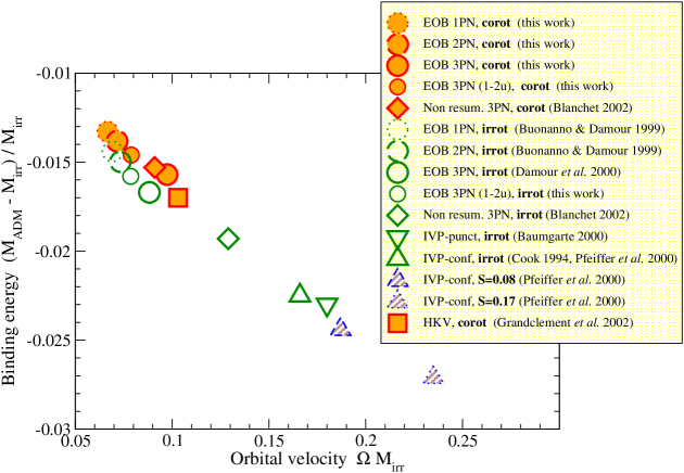
Figure 3: Maximum binding energy configurations (LSO) obtained with various analytical and numerical methods. Empty (resp. filled) symbols denote irrotational (resp. corotating) systems. ‘EOB 3PN’ denotes the computation performed with the Padé approximant $\overline{A}(u,{\hat{a}}^{2})$ given by Eq. (14), whereas ‘EOB 3PN (1-2u)’ corresponds to the $\overline{A}^{\prime}(u,{\hat{a}}^{2})$ form given by Eq. (15). References are as follows: Blanchet 2002 B02 ; Buonanno & Damour 1999 BD00 ; Damour et al. 2000 DJS00 ; Baumgarte 2000 baumgarte ; Cook 1994 cook ; Pfeiffer et al. 2000 PfeifTC00 ; Grandclément et al. GGB2 .

III.2 Characteristics of the LSO

Figure 3 compares various analytical and numerical estimates of the maximum binding energy $(E_{\rm real}/M_{\rm irr})-1$, together with the corresponding dimensionless angular velocity $M_{\rm irr}\,\Omega$, along sequences of circular orbits of equal-mass black holes. Note that some sequences are corotating while others are irrotational. Several interesting lessons can be drawn from Fig. 3. The first one is that the analytical (EOB) results show that the effect of the corotation is quite small. [The reason for this smallness is discussed in detail below.] In fact, the corotation effects are smaller or comparable to the differences induced by making other changes in the treatment of the problem (like using a different resummation method for the basic EOB potential $A(u)$, or working at the 2PN approximation instead of the 3PN one).

Another important lesson drawn from Fig. 3 concerns the PN robustness of the EOB estimates (i.e. their stability under a change of PN accuracy): Indeed, we have compared the results corresponding to the 1PN approximation of the EOB potential $\overline{A}(u)$, namely

$$\overline{A}^{\rm 1PN}(u)=1-2u+\widehat{a}^{2}\,u^{2}\,,$$ (37)

to its 2PN approximation

$$\overline{A}^{\rm 2PN}(u)=P_{2}^{1}[1-2u+\widehat{a}^{2}\,u^{2}+2\,\nu\,u^{3}]\,,$$ (38)

and to its 3PN approximation (14) (with $a_{4}(\nu)$ given by Eq.(11)).

We see that, on the scale of the differences between the various estimates, and in particular, on the scale of the differences of the various numerical results among themselves, the EOB method yields rather close results at all PN approximations. This is one of the signs of the good resummation properties of the EOB method, and is to be contrasted with the much poorer behavior (under a change of PN accuracy) of the other analytical methods of estimating LSO characteristics such as: the direct use of PN-expanded equations of motion LW90 (as discussed in Table II of KWW93 ), the use of PN-expanded Hamiltonians (as discussed in WS and Buona02 ; see, e.g., Fig. 3 of Buona02 ), the $E$-method (discussed in Table I, Table VII and Fig. 5 of DIS98 , and in Fig. 3 of B02 ), the $e$-method (discussed in DIS98 and DJS00 ) or the $j$-method DJS00 .

For comparison purposes, we have included in Fig. 3 the (irrotational and corotating) analytical predictions recently derived by using the the non-resummed $E$-method at the 3PN level B02 . We note that the prediction of the non-resummed $E$-method for the irrotational LSO angular velocity is $46$% larger than the corresponding EOB prediction. The fact that the $E$-method yields, at 3PN, significantly larger values of $({\Omega M_{\rm irr}})_{\rm LSO}$ than the EOB one, in the equal-mass case, is not surprising in view of the fact that it already did so in the “test mass limit” ($\nu\to 0$), i.e. when one mass is much smaller than the other one. Let us introduce the dimensionless ratios, $a=(\Omega M_{\rm irr})/{(\Omega M_{\rm irr})}^{\rm exact},b=(E_{\rm real}/M_{\rm irr}-1)/{(E_{\rm real}/M_{\rm irr}-1)}^{\rm exact}$, for LSO characteristics. In the test-mass limit (where the exact answers are known), the EOB method yields exact results, i.e. $(a,b)=(1,1)$ at all PN levels. By contrast, the $E$-method yields DIS98 ; DJS00 : $(8,2.914)$ at 1PN, $(1.824,1.315)$ at 2PN, and $(1.275,1.103)$ at 3PN. This monotone approach, from upwards, towards the exact answer is linked to the signs of the expansion coefficients of the function $E(x)$. As these signs remain the same for all values of $\nu$ one also expects the $E$-method to yield overestimates of $\Omega$ and $E_{\rm real}$ in the equal-mass case. It is, in our opinion, an important feature of the EOB method (which is shared by none of the non-resummed PN approaches) that it yields exact results when $\nu\to 0$, and “robust” results (not depending very much on the PN accuracy used) when $\nu$ is not zero, and notably when $\nu=1/4$ (equal-mass case). On the other hand, in the equal-mass corotating case, the 3PN-level $E$-method predicts a maximal binding configuration which is within 10 % (both for $\Omega$ and $E_{\rm real}$) of the 3PN EOB prediction, as well as of the HKV numerical results B02 . In view of the test-mass-limit behavior, and of the rather large difference in the estimates of the effects linked to corotation (see the distance between the diamonds in Fig. 3, and the discussion in the next subsection), we view this 10 % agreement as accidental.

Though the 1PN, 2PN and 3PN results are much closer in the EOB approach than in other (less resummed) PN approaches (compare, e.g., the results here with Fig. 3 of Ref. B02 whose 1PN predictions would not fit on our Figure 3 above), one, however, notices that there is somewhat of a jump between the 1PN and 2PN results on one hand, and the 3PN ones on the other hand. This is due to the largish positive numerical value of $a_{4}^{\rm GR}$, Eq. (11). Indeed, a positive $a_{4}$ means a repulsive term in the radial Hamiltonian. This (relative) “repulsion” allows the LSO to move inwards, towards more binding. The largish positive value of $a_{4}^{\rm GR}$ (when $\nu=1/4$) has thereby a somewhat significant effect on the maximal binding (towards more binding). One should, however, remember that Ref. BD00 has shown that the location of the LSO was blurred by radiation damping effects. The difference between 2PN and 3PN predictions is probably barely observable in the GW signal emitted by coalescing black holes. [See DIJS for a discussion of the observability of the various parameters entering the EOB framework, and for an estimate of the plausible value of the 4PN term $a_{5}^{\rm GR}$ and its effect on the LSO.]

But the most striking feature of Fig. 3 is, on the one hand, the closeness between the EOB results and the numerical results of GGB2 , and on the other hand, the huge difference between the latter results, and the numerical results of the conformal imaging cook ; PfeifTC00 or puncture baumgarte IVP methods.

To complete the information displayed in Fig. 3 we give in Table 1 the corresponding numerical data. Table 1 gives also data corresponding to several possible alternative versions of the basic function $\overline{A}(u)$ used in the EOB approach (see Eqs.(15)-(17)). In particular, note that all the Padé alternatives ($\overline{A},\overline{A}^{\prime\prime},\overline{A}^{\prime\prime\prime}$) yield very close results. This is further illustrated in Fig. 4. Even the “factorized Taylor” version ($\overline{A}^{\prime}$) (which incorporates a rather brutal way of forcing $\overline{A}(u)$ to have a simple zero) gives (as is clear from Fig. 3) results which are in good agreement both with other 3PN EOB results and with the HKV ones. Though we believe that such a “factorized Taylor” version of $\overline{A}(u)$ is, a priori, not as good as the various Padé versions, we included it because we think that its difference with the Padé results gives a plausible upper limit of the “error bar” on the 3PN EOB predictions. For instance, we think that a plausible range for the correct maximal binding energy is $E^{\rm corot}_{\rm real}/M_{\rm irr}-1=-0.0157\pm 0.0011$, in the corotating case, and $E^{\rm irrot}_{\rm real}/M_{\rm irr}-1=-0.0167\pm 0.0009$ in the irrotational one. Note also that Table 1 (and Fig. 3) include no data corresponding to the straightforward Taylor version (12) [truncated at ${\cal O}(u^{5})$]. Indeed, the qualitatively different behavior of $A^{\rm Taylor}(u)$ (without simple zero, see Fig. 1 above) prevents the presence of a minimum along the curve $E(\Omega)$, as shown in Fig. 4. The latter Figure illustrates the fact that, even within the EOB approach, there is a contrast between the closeness of the Padé-type predictions and the dispersion of the Taylor-type ones (straightforward Taylor and factorized Taylor). Again, we can use the distance (visually displayed in Fig. 4) between Padé results and Taylor ones to define a (two-sided) “error bar” on the EOB Padé predictions.

Table 1: Parameters of the LSO configuration according to various methods. Unless otherwise noticed, PN computations correspond to the EOB approach with $\overline{A}(u)$ functions given in the text and with the 3PN parameter $a_{4}$ set to $4.672$, see Eq. (11). For $\overline{A}^{\prime\prime\prime}(u,\widehat{a}^{2})$, we have used $a_{5}=-3$. The relative “orbital” binding energy $e$ is defined by Eq. (42).

Method	$\Omega M_{\rm ir}$	$M_{\rm ADM}/M_{\rm irr}-1$	$J/M_{\rm irr}^{2}$	$L/M_{\rm irr}^{2}$	$u$	$\hat{a}$	$m_{1}/m_{1}^{\rm irr}$	$e$
1PN corot	0.0667	-0.0133	0.907	0.846	0.164	0.108	1.0019	-0.0152
2PN corot	0.0715	-0.0138	0.893	0.828	0.173	0.115	1.0022	-0.0160
3PN corot $\overline{A}(u,\widehat{a}^{2})$	0.0979	-0.0157	0.860	0.774	0.220	0.149	1.0037	-0.0193
3PN corot $\overline{A}^{\prime}(u,\widehat{a}^{2})$	0.0789	-0.0146	0.876	0.805	0.186	0.125	1.0026	-0.0172
3PN corot $\overline{A}^{\prime\prime}(u,\widehat{a}^{2})$	0.0999	-0.0157	0.859	0.773	0.223	0.151	1.0037	-0.0193
3PN corot $\overline{A}^{\prime\prime\prime}(u,\widehat{a}^{2})$	0.1055	-0.0160	0.856	0.766	0.233	0.157	1.0041	-0.0200
3PN corot non resum. B02	0.091	-0.0153
HKV corot GGB2	0.103	-0.017	0.839
1PN irrot BD00	0.0692	-0.0144	0.866	0.866	0.167	0	1	-0.0144
2PN irrot BD00	0.0732	-0.0150	0.852	0.852	0.174	0	1	-0.0150
3PN irrot $\overline{A}(u,0)=\overline{A}^{\prime\prime}(u,0)$ DJS00	0.0882	-0.0167	0.820	0.820	0.202	0	1	-0.0167
3PN irrot $\overline{A}^{\prime}(u,0)$	0.0786	-0.0158	0.834	0.834	0.185	0	1	-0.0158
3PN irrot $\overline{A}^{\prime\prime\prime}(u,0)$	0.0898	-0.0168	0.817	0.817	0.205	0	1	-0.0168
3PN irrot non resum. B02	0.129	-0.0193	0.786
IVP-punct irrot baumgarte	0.18	-0.023	0.737
IVP-conf irrot PfeifTC00	0.166	-0.0225	0.744

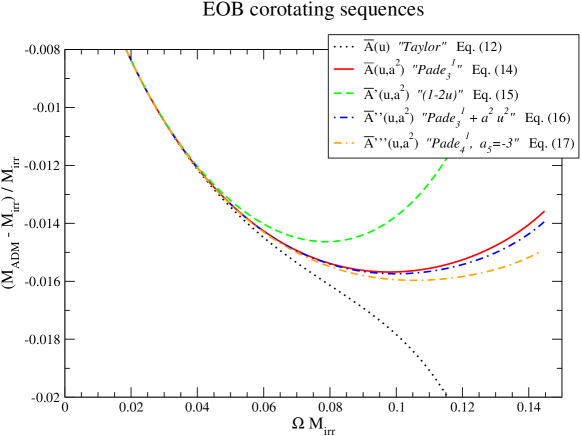
Figure 4: Binding energy as a function of the orbital velocity, for the various alternatives to the $\overline{A}(u,{\hat{a}}^{2})$ function.

III.3 Spin effects in the determination of the LSO

Before considering in more detail the characteristics of the circular orbits around the LSO, it is interesting to discuss the reason why there is such little difference between the irrotational and corotating cases. Indeed, if we consider, say, our preferred EOB potential $\overline{A}(u,{\hat{a}}^{2})$, at the 3PN approximation, Table 1 shows that the maximum corotating binding energy is $-0.0157$, while the irrotational value is $-0.0167$. The difference is only $1\times 10^{-3}$. This difference is about 4 times smaller than the difference obtained in B02 which used a non-resummed PN approach. We are going to see that the relatively large difference obtained in this non-resummed PN approach is rooted in the (truncated) perturbative nature of this approach.

One can distinguish two leading contributions to the difference in binding energy: (i) a contribution linked to the (kinetic) rotational energies of the spinning black holes, and (ii) a contribution linked to the spin-orbit interaction. [There are also mixed terms involving, e.g., products of the spin kinetic energy with orbital effects, but one can check that they are numerically smaller.] In the language of the present paper, the first contribution is essentially embodied in the factor $m_{1}/m_{1}^{\rm irr}$ in the first Eq.(III.1) above. For corotating configurations, Eq.(34) above approximately yields $\widehat{a}_{1}=\widehat{a}_{2}=2\omega$ where $\omega\equiv M_{\rm irr}\Omega\approx M\Omega$. This yields $m_{1}/m_{1}^{\rm irr}-1\approx\omega^{2}/2$. Numerically, we have (for the irrotational 3PN case; see Table 1), $\omega\approx 0.09$, so that $m_{1}/m_{1}^{\rm irr}-1\approx 4\times 10^{-3}$. This is essentially the difference “corotating - irrotational” in binding energy obtained in B02 , because, within the non-resummed PN approach of B02 , the kinetic-spin contribution largely dominates over the spin-orbit interaction energy. We wish, however, to point out that there are consistency problems in the application of straightforward (truncated) PN-expanded methods to the determination of the effect of the spin-orbit interaction on the maximum binding energy. By contrast, we shall see that the EOB estimate of the same quantity has no consistency problems, and happens to be much larger and to nearly cancel the kinetic-spin contribution.

To have a common language between the two approaches (straightforward PN approach and EOB approach), let us write the Hamiltonian of a binary system as $H=H_{0}(r,L)+H_{1}(r,L,S)$, where $H_{1}=2\,LS/r^{3}$ is the spin-orbit interaction to linearized order BOC . Here, $S=\sigma_{1}S_{1}+\sigma_{2}S_{2}$ denotes the effective spin (with the same notation as above for $\sigma_{1},S_{1}$,etc.). We only consider the aligned case where the spins are parallel to the orbital angular momentum $L$. [Here, we consider the masses as given parameters, because we treat separately the effects linked to the kinetic energies of the spins.] To first order in $H_{1}$, the energy along sequences of circular orbits, as a function of the radial coordinate $r$, (obtained by solving $\partial H/\partial r=0$ so as to get $L=L(r)$), can be written as $H^{(r)}[r]=H_{0}^{(r)}[r]+H_{1}^{(r)}[r]$, where $H_{0}^{(r)}[r]$ is the answer corresponding to $H_{0}(r,L)$ and where the first-order correction linked to $H_{1}(r,L)$ ( we consider $S$ as a spectator variable which will be, at the end, replaced by a function of $r$ obtained from the corotation condition) reads:

$$H_{1}^{(r)}[r]=\left[H_{1}(r,L)-\frac{\partial_{L}\,H_{0}(r,L)}{\partial_{rL}^{2}\,H_{0}(r,L)}\,\partial_{r}\,H_{1}(r,L)\right]_{L=L_{0}(r)}\ .$$ (39)

Here, $L_{0}(r)$ is the angular momentum along the radial sequences of circular orbits defined by $H_{0}(r,L)$. If one then asks (as in KWWR ; B02 ) for the variation of the energy as a function of the orbital frequency $\Omega(r)=[\partial\,H(r,L)/\partial\,L]_{L=L(r)}$, one finds $H^{(\Omega)}[\Omega]=H_{0}^{(\Omega)}[\Omega]+H_{1}^{(\Omega)}[\Omega]$, where $H_{0}^{(\Omega)}[\Omega]$ is the answer corresponding to $H_{0}$ and where the $H_{1}$-related correction reads:

$$H_{1}^{(\Omega)}[\Omega]=\left[H_{1}^{(r)}-\frac{d\,H_{0}^{(r)}/dr}{d\,\Omega_{0}(r)/dr}\left(\partial_{L}\,H_{1}-\frac{\partial_{L}^{2}\,H_{0}}{\partial_{rL}^{2}\,H_{0}}\,\partial_{r}\,H_{1}\right)\right]\ .$$ (40)

Here, the brackets mean that one evaluates a quantity for $L=L_{0}(r)$ and then changes variables via: $r=r_{0}(\Omega)$. Having these results in hand, we can now compare the straightforward (non-resummed) PN approach to the EOB one. The non-resummed PN approach considers that $H_{1}$ is already of high-PN order, so that, in all the $H_{1}$-related corrections above one can replace the zeroth-order Hamiltonian $H_{0}$ by its Newtonian approximation. Applying then the formulas above to the spin-orbit Hamiltonian ($H_{1}\propto Lr^{-3}$) yields the simple results: $H_{1}^{(r)}=-\frac{1}{2}\,[H_{1}]$ and $H_{1}^{(\Omega)}=-\frac{2}{3}\,[H_{1}]$, where the brackets indicate that $H_{1}$ should be evaluated along the considered sequence (and expressed in terms of the corresponding variable). [One easily checks that the result for $H_{1}^{(\Omega)}$ is equivalent to the formula derived in KWWR and used in B02 .]

It is interesting to note that the results are numerically different. To have such a difference is fine far from the LSO (and the PN calculations are both valid there), but it is problematic near the LSO. Let us first recall the standard approximate estimate (valid to linear order in the perturbation) of the minimum of a function of the type $f(x)=f_{0}(x)+f_{1}(x)$ where $f_{0}(x)$ has a local minimum at $x_{\min}$: when working to first order in $f_{1}$ one easily gets $f_{\min}\approx f_{0}(x_{\min})+f_{1}(x_{\min})$. Applying this general result to the case at hand, we simply get the spin-orbit (SO) contributions at maximum binding by evaluating the corrections $H_{1}^{(r)}$ or $H_{1}^{(\Omega)}$ at the zeroth-order (irrotational) LSO. We thereby get different values (by a factor $4/3$). However, it is physically (and mathematically) inconsistent to get different estimates of the SO-induced change in maximum binding energy. Indeed, one is considering the same quantity (the energy) expressed in terms of different (gauge-invariant, monotonically varying) independent variables: $r$ or $\Omega$. The numerical value of the minimum of this quantity should be the same (even if is reached at a different value of the independent variable). This consistency problem is linked to the perturbative nature of the (non-resummed) PN approach which (self-consistently) treats the spin-orbit effects as being of higher PN order, and truncates away (most of) the “mixed” terms involving products of the PN contributions to $H_{0}$ with SO effects. Note, a contrario, that the consistency of the non-resummed PN treatment would be recovered if one were to keep all those mixed terms.

By contrast, the EOB approach is immune to such consistency problems. Indeed, the EOB approach does not approximate $H_{0}$ in the correction terms by its Newtonian expression. It, instead, uses the full (non-perturbative) expression Eq.(13). This value of $H_{0}$ consistently contains an LSO, i.e. a value of $r$ (and $\Omega$) where $dH_{0}^{(r)}/dr$ vanishes. One then sees that, when evaluating (in the approximate way indicated above) the change in the maximum binding induced by $H_{1}$, the last correction term in $H_{1}^{(\Omega)}$ vanishes, so that we get (whatever be the independent variable used) $\delta E_{\rm LSO}^{\rm EOB}={H_{1}^{(r)}}_{\rm LSO}={H_{1}^{(\Omega)}}_{\rm LSO}$. Moreover, using the full expression Eq.(13) for $H_{0}$ one gets the explicit expression (where $u=M/r$):

$$\delta\,E_{\rm LSO}^{\rm EOB}=\{1-3\,A/(2\,A+u\,\partial_{u}\,A)\}\,[H_{1}]\ .$$ (41)

This value depends on the expression used for the EOB potential $A(u)$, and, thereby, on the corresponding location of the LSO. If we consider, for simplicity, the limit $\nu\to 0$, we can use the simple form $A(u)=1-2u$, and the corresponding LSO location: $u_{\rm LSO}=1/6$. This then yields $\delta E_{\rm LSO}^{\rm EOB}=-[H_{1}]$. We see that the EOB approach gives a larger contribution than both the straightforward PN methods discussed above. This larger value is due to the fact that the EOB approach is non perturbative in that it treats the effective potential $A(u)$ exactly near the LSO.

Let us introduce the dimensionless “orbital” binding energy

$$e\equiv\frac{E-M}{M}=\frac{1}{4}\widehat{E}-1=\frac{1}{4}\frac{E_{\rm real}}{\mu}-1=\frac{m_{1}^{\rm irr}}{m_{1}}\frac{M_{\rm ADM}}{M_{\rm irr}}-1\ .$$ (42)

Inserting the explicit value of the spin-orbit Hamiltonian (and consistently using $r_{\rm LSO}=6M$) finally gives the following estimate for the spin-orbit modification of $e$, in the “test-mass” limit $\nu\to 0$:

$$\delta^{\rm SO}\,e_{\rm LSO}=-\sqrt{3}\ 6^{-3}\,\nu_{4}\,\widehat{a}=-0.802\times 10^{-2}\,\nu_{4}\,\widehat{a}\ .$$ (43)

Here, $\nu_{4}\equiv 4\nu$ and $\widehat{a}$ denotes the effective dimensionless spin parameter $S/M^{2}$. The numerical coefficient $0.802$ is about twice larger than the corresponding result obtained in B02 . Note that this coefficient is consistent with the small $\nu$ limit of the result written in Eq.(4.1) of D01 . The latter equation then shows that, in the equal-mass case (of interest here), $\nu=1/4$, i.e. $\nu_{4}=1$, the numerical coefficient giving the SO-induced change of $e_{\rm LSO}$ is further enhanced (by a factor 1.888) to the value $\delta^{\rm SO}\,e_{\rm LSO}=-1.52\times 10^{-2}\widehat{a}$. Actually, the data in Table II of D01 show that the latter result is valid only for values of $\widehat{a}$ smaller than $0.1$. For the value $\widehat{a}\approx 0.15$ relevant to us (see Table 1 above), nonlinear effects in $\widehat{a}$ further enhance the change in binding energy. Interpolating between the numerical data given in Table II of D01 one can see that a better estimate of $e$ for $\widehat{a}\approx 0.15$ is $e_{\rm LSO}\approx-0.0197$. Compared to the value without spin-orbit contribution, $e_{\rm LSO}=-0.0167$, this yields a SO-related modification equal to $\delta^{\rm SO}\,e\simeq-0.30\times 10^{-2}$.

Finally, we conclude that the EOB approach gives (at 3PN): (i) an increase of $E_{\rm LSO}/M_{\rm irr}$ due to the kinetic energy of the spinning black holes of order $+4\times 10^{-3}$, and a decrease linked to spin-orbit effects (as estimated within the EOB framework) of order $-3\times 10^{-3}$. The net result is that $E_{\rm LSO}/M_{\rm irr}$ increases only by $+1\times 10^{-3}$. This analysis has clarified why and how the EOB approach yields a rather small final effect for the difference between the irrotational case and the corotating one. We view this result as a confirmation of the generic robustness of the EOB approach. By contrast, we view the significantly larger change predicted by non-resummed PN approaches as further confirmations of the generic lack of robustness of non-resummed PN methods. An interesting lesson of this comparison is that the larger SO-related changes predicted by the EOB approach are crucially linked to its non perturbative nature.

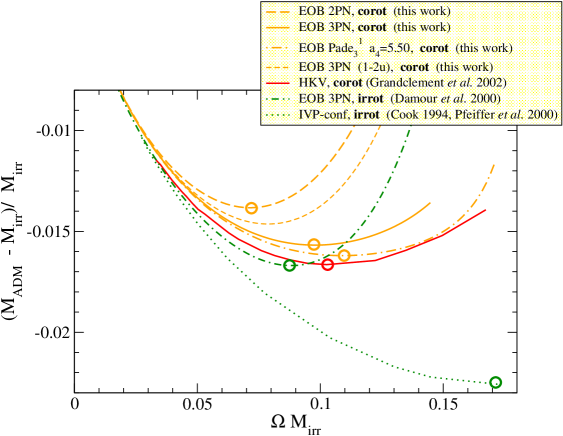
Figure 5: Binding energy as a function of the orbital angular velocity, according to various analytical and numerical methods.

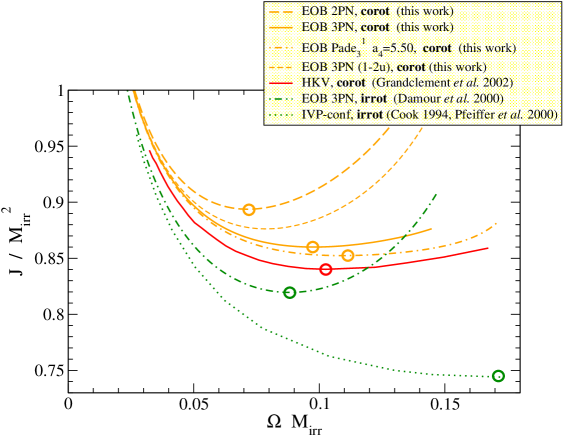
Figure 6: Total angular momentum as a function of the orbital angular velocity, according to various analytical and numerical methods.

III.4 Evolutionary sequences

As we said above, the LSO characteristics do not embody the really useful information contained in the various approximations to binary black holes dynamics. To have a complete hold on the two-body dynamics one would need to compare the Hamiltonians, $H(r,p_{r},L,S_{a})$. The EOB method provides such a complete description (which allows it to describe not only the adiabatic inspiral but also the crucial transition to the plunge). However, numerical methods do not give access to such a multi-variable function. As a makeshift we can at least compare various functions of one variable linked to the two-body dynamics. In Fig. 5 we plot various analytical and numerical estimates of the binding energy of circular orbits versus the orbital frequency, while Fig. 6 plots the total angular momentum $J$. These figures show that the methods that led to good agreement for LSO characteristics in Fig. 3, also lead to good agreement for all circular orbits, and all available dynamical quantities. We have also included in these figures the results coming out of the straightforward truncation of the $A$-function, Eq. (12). We see that it agrees rather well (compared, say, with the conformal-imaging or puncture data) with the helical Killing vector (HKV) data nearly up to the LSO.

If we remember that Ref. BD00 has shown that, a little bit above the normal (adiabatic) LSO, radiation damping effects dominate over the “restoring” radial potential, it is very plausible that even the pure Taylor EOB function $\overline{A}(u)$ would lead to a GW signal essentially indistinguishable from the one obtained from a Padé-resummed function $\overline{A}(u)$. Note that Figs. 5 and 6 confirm the messages of Fig. 3: the main feature is a nice agreement of all versions of EOB and HKV results versus a significant difference with the conformal-imaging or puncture results. When looking at the finer structure of the EOB predictions one sees that the 3PN predictions are much closer to the HKV data than the 2PN ones.

As we said above, the multi-parameter “flexibility” of the EOB approach $(a_{4}(\nu),a_{5}(\nu),a_{6}(\nu),\ldots)$ can be exploited, to further improve, if deemed necessary, the agreement with numerical data. For instance, we have played with the addition of $a_{5}(\nu)$ and found that, with the Padé resummation (17), a value $a_{5}\left(\frac{1}{4}\right)\simeq\,-3$ further improves the agreement with HKV data. However, we do not consider such a best fit value of $a_{5}(\nu)$ as significant at this stage. Another interesting “robustness” exercise consists in modifying the general relativistic (GR) prediction (10) for the 3PN coefficient (10). We recall that, from the recent dimensional continuation calculation of DJS01 , the GR value should be, when $\nu=\frac{1}{4}$, $a_{4}^{\rm GR}=4.672$ (see Eq. (11)). By varying $a_{4}$ (without adding any further terms $a_{5}(\nu),a_{6}(\nu),\ldots$) we found that a value which provides a slightly better fit is $a_{4}\left(\frac{1}{4}\right)=5.50$. The corresponding curves are plotted in Figs. 5 and 6. On the other hand, note that the value $a_{4}=0$, corresponding to the 2PN approximation only, noticeably worsens the agreement with the HKV data. In all cases, the reader should notice that the binding energy differences linked to these different choices for the 3PN contribution $a_{4}$ remain small compared with the dispersion among all numerical results.

IV Conclusions

IV.1 Robustness of the EOB method

The main conclusions of this work are the following. We have confirmed the robustness of the effective one-body (EOB) approach to binary black hole dynamics. The various ways of resumming the crucial EOB radial function $\overline{A}(u)$ exhibited in Figs. 1 and 2 lead to predictions for the binding energy and the angular momentum as functions of orbital frequency, which are very close to each other, see Figs. 3, 5 and 6, and Table 1. Even the “non resummed” function $\overline{A}(u)$ (upper curve in Fig. 1) leads to dynamical predictions which are quantitatively close to the “resummed” predictions up to the last orbits before the Last Stable (circular) Orbit (LSO) (see Figs. 5 and 6). We have argued that it would probably yield indistinguishable waveforms if used, as in BD00 , to study the transition between inspiral and plunge. [However, if one wishes, as in BD00 , to continue the description of the plunge nearly down to coalescence we expect that a non resummed $\overline{A}(u)$ will quickly lead to problems and to strong deviations from the results obtained from various resummed $\overline{A}(u)$.] Another robustness feature of the EOB approach is its good post-Newtonian (PN) convergence properties. This was illustrated in Figs. 3, 5 and 6 where the 1PN, 2PN and 3PN predictions are seen to be all much closer to the helical Killing vector (HKV) data than to the other numerical data. Note, however, that the best agreement with HKV data is obtained for the 3PN prediction. We emphasized also the consistency (and robustness) of the EOB approach in the treatment of the changes induced by spin effects. This contrasts with non-resummed PN approaches which predict different changes when one uses different parameters to run along a corotating sequence.

IV.2 Extension of the EOB method to corotating systems

The most novel aspect of the present work is that we have shown how to apply to corotating sequences the recently defined D01 extension of the EOB approach to spinning black holes. The effects linked to the spins turn out, finally, to be rather small. For instance, they are significantly smaller than the effect of using the 3PN-accurate EOB Hamiltonian instead of a 2PN-accurate one, see Fig. 3. We discussed the reasons behind this behavior (essentially a near cancellation between an energy increase linked to the spin kinetic energy and an energy decrease linked to the rather strong spin-orbit interaction predicted by the EOB method).

IV.3 Good agreement between EOB and HKV results

Our findings fully confirm what was announced in GGB2 : the new HKV numerical data are much closer to analytical results than previous numerical data. At face value, this is a very encouraging fact which suggests that one can now implement the philosophy which was at the basis of the EOB approach BD00 : to use a (resummed) analytical approach to describe binary black holes not only during early inspiral (which was previously thought to be the only possible domain of validity for an analytical approach), but also during late inspiral and, most importantly, during the transition between inspiral and plunge. Numerical relativity techniques can then be used only for describing the rest of the plunge and the coalescence. [As noted in baker one might also simplify matters by describing the end of the coalescence by the “close limit approximation”.] A crucial requirement for successfully merging together analytical and numerical results is to be able to match the analytical description just after the last stable orbit (LSO) with suitable numerical initial data. This paper is an encouraging step in this direction, in view of the robust and close agreement between EOB results and HKV ones.

However, this agreement raises many questions. A first question is linked to the “approximations” used in the present implementation of the HKV philosophy. Indeed, though this method is not, in principle, limited to conformally flat data, its present implementation has, for simplicity, imposed conformal flatness of the spatial metric, and has reduced the ten equations (for ten unknowns) to solve to a subset of five equations (for five unknowns). The reason why this restriction is problematic is that, from the analytical side, the values of the successive coefficients in the various functions entering the EOB formalism depend quite sensitively on the exact form of the metric, and, in particular, on the fact that it is not conformally flat. For instance, it was shown in DJS00 that both the “effective potential” $A(u)$, and the energy map (1), are modified, at the 2PN approximation, if one truncates Einstein equations to impose conformal flatness. The corresponding modification at the 3PN approximation is currently not known. However, these modifications might turn out not to be critical in view of the robustness of the EOB predictions. Fig. 3 shows that even if we use the EOB Hamiltonian at the 1PN approximation (which, in fact, essentially coincides with the “Newtonian” approximation, i.e. the EOB reformulation of the “test-mass approximation”), one is much closer to HKV data than to the other numerical data.

IV.4 Plausible explanation of the disagreement with IVP results

The most important question posed by the agreement analytical/HKV is to understand why the IVP approaches give (consistently among themselves) drastically different results. After all, both types of numerical approaches use (at present) the same simplification of spatial conformal flatness $(\gamma_{ij}=\psi^{4}\,\delta_{ij})$, and they both numerically construct solutions to the Hamiltonian and momentum constraints (approximate solution to the momentum constraint for HKV). Seen from this technical point of view, the difference between the two schemes lies in the way of solving the momentum constraint. In the IVP method cook ; PfeifTC00 ; baumgarte , it is solved by means of a simple ansatz (Bowen-York extrinsic curvature BowenY80 or its isometric version KulkaSY83 ) for the second fundamental form $K_{ij}$ whose weak-field limit is reasonable, while in the HKV method GGB1 ; GGB2 one determines an essentially unique solution for $K_{ij}$ by the requirement that it be induced by restricting a helically-symmetric spacetime to a Cauchy hypersurface (see also Cook02 for a discussion). We think that the basic physical difference between the two approaches, which underlies their drastically different predictions, is the following. Though it must be admitted that the imposition of a helical symmetry can only be an approximation, it is a physically well motivated approximation which has the great virtue of selecting a specific solution of the constraints. This is very similar to what happens in the post-Newtonian schemes, especially in their ADM version. Indeed, in the Hamiltonian ADM approach one uses (when dealing with the near-zone field) the post-Newtonian ansatz $(c^{-1}\,\partial_{t}\,h\ll\partial_{x}\,h)$ to derive and solve an iterative set of coupled elliptic equations for $\gamma_{ij}$ and $K_{ij}$. This selects a specific solution of the constraints. Intuitively, one can think of this (essentially) unique solution selected by the PN method as the only solution of the constraints which contains the “right” amount of free gravitational wave (GW) data $(h_{ij}^{TT},\pi_{TT}^{ij})$ which has been generated by the many previous orbits of the system, and which has therefore reached a quasi-stationary state. Any other amount of GW data would be a priori allowed at a specific moment of time but would not correspond to a quasi-stationary state, and would therefore be expected to “fly away” with the velocity of light, i.e. to evolve in a violently non quasi-stationary way, with $c^{-1}\,\partial_{t}\,h\sim\partial_{x}\,h$ instead of $c^{-1}\,\partial_{t}\,h\ll\partial_{x}\,h$. We think that this PN understanding of the selection, by reduction to elliptic equations, of a specific “quasi-stationary” solution applies, mutatis mutandis, to the HKV approach. The imposition of a helical Killing vector selects the only “quasi-stationary” solution corresponding to a steady situation generated by a slow inspiral, while the arbitrary choice, in the other methods, of a technically simple solution of the momentum constraint corresponds to a drastically non-steady state, containing a wrong amount of free GW data, which is expected to “fly away” as soon as one tries to evolve the system in time. If this view is correct, it diminishes the signification of the “effective potential” approach applied to the initial data of cook ; PfeifTC00 ; baumgarte . Indeed, these data correspond to a non-steady state to which it is incorrect to apply any energy minimization principle.

IV.5 Fitting the EOB Hamiltonian to numerical data

We have started to exploit the “flexibility” of the EOB approach (already emphasized in D01 ), i.e. the use of the expansion coefficients appearing in the EOB approach as parameters to be fitted. For instance, Figs. 5 and 6 exhibit the dynamical predictions obtained from a modified 3PN coefficient, $a_{4}^{\rm best\,fit}\left(\frac{1}{4}\right)\simeq 5.50$ instead of $a_{4}^{\rm GR}\left(\frac{1}{4}\right)\simeq 4.67$. The modified value of $a_{4}$ leads to a better agreement with the HKV data. As we are not adding any higher PN contributions, $a_{5}(\nu)u^{5}+a_{6}(\nu)u^{6}+\ldots$, such a best fit value for $a_{4}$ can be viewed as a way of mimicking the effect of such (missing) higher PN terms.

We resisted the temptation to (introduce and) vary more $a_{n}(\nu)$ parameters up to getting a really close agreement with HKV data, because, at this stage, such a formal exercise would not be justified. It is, however, important to keep in mind the suggestion made in D01 that a suitable “numerically fitted” EOB Hamiltonian may be a very useful tool for combining the advantages of analytical and numerical methods. If we look ahead to the problem of exploring the dynamics of two arbitrarily spinning black holes, one will have to face an extremely large parameter space. It seems clear that numerical relativity will not be able (before many years) to cover densely this parameter space. On the other hand, one can use some sparse numerical data to determine free parameters introduced in a generalized EOB Hamiltonian. Then this “numerically fitted” EOB Hamiltonian can be used to interpolate between the sparse numerical data.

References

- (1) V.M. Lipunov, K.A. Postnov and M.E. Prokhorov, New Astron. 2, 43 (1997).
- (2) E.E. Flanagan and S.A. Hughes, Phys. Rev. D 57, 4535 (1998).
- (3) P.R. Brady, J.D.E. Creighton and K.S. Thorne, Phys. Rev. D 58, 061501 (1998).
- (4) S.F. Portegies Zwart and S.L. McMillan, Astrophys. J. 528, L17 (2000).
- (5) T. Damour, B.R. Iyer and B.S. Sathyaprakash, Phys. Rev. D 62, 084036 (2000); and Phys. Rev. D 63, 044023 (2001).
- (6) A. Buonanno and T. Damour, Phys. Rev. D 59, 084006 (1999); and Phys. Rev. D 62, 064015 (2000).
- (7) T. Damour and N. Deruelle, Phys. Lett. A 87, 81 (1981); T. Damour, C.R. Séances Acad. Sci. Ser. 2, 294, 1355 (1982)
- (8) P. Jaranowski and G. Schäfer, Phys. Rev. D 57, 7274 (1998); and Phys. Rev. D 60, 124003 (1999).
- (9) T. Damour, P. Jaranowski and G. Schäfer, Phys. Rev. D 62, 021501 (R) (2000); Phys. Rev. D 63, 044021 (2001); and Phys. Lett. B 513, 147 (2001).
- (10) L. Blanchet and G. Faye, Phys. Lett. A271, 58 (2000); and Phys. Rev. D 63, 062005 (2001); V.C. de Andrade, L. Blanchet and G. Faye, Class. Quant. Grav. 18, 753 (2001).
- (11) L. Blanchet, T. Damour, B.R. Iyer, C.M. Will and A.G. Wiseman, Phys. Rev. Lett. 74, 3515 (1995); L. Blanchet, T. Damour and B.R. Iyer, Phys. Rev. D 51, 5360 (1995); C.M. Will and A.G. Wiseman, Phys. Rev. D 54, 4813 (1996); L. Blanchet, Phys. Rev. D 54, 1417 (1996).
- (12) L. Blanchet, Class. Quantum Grav. 15, 113 (1998); L. Blanchet, B.R. Iyer, and B. Joguet, Phys. Rev. D 65, 064005 (2002).
- (13) T. Damour, B.R. Iyer and B.S. Sathyaprakash, Phys. Rev. D 57, 885 (1998).
- (14) T. Damour, P. Jaranowski and G. Schäfer, Phys. Rev. D 62, 084011 (2000); and Phys. Rev. D 62, 044024 (2000).
- (15) L. Blanchet, Phys. Rev. D, in press (gr-qc/0112056).
- (16) G.B. Cook, Phys. Rev. D 50, 5025 (1994).
- (17) H.P. Pfeiffer, S.A. Teukolsky, and G.B. Cook, Phys. Rev. D 62, 104018 (2000).
- (18) T.W. Baumgarte, Phys. Rev. D 62, 024018 (2000).
- (19) A. Buonanno, to appear in the Proceedings of 4th Edoardo Amaldi Conference on Gravitational Waves, Perth, Australia, 8-13 July 2001 (preprint gr-qc/0203030).
- (20) J. Baker, B. Brügmann, M. Campanelli, C.O. Lousto, and R. Takahashi, Phys. Rev. Lett. 87, 121103 (2001).
- (21) E. Gourgoulhon, P. Grandclément, and S. Bonazzola, Phys. Rev. D 65, 044020 (2002).
- (22) P. Grandclément, E. Gourgoulhon, and S. Bonazzola, Phys. Rev. D 65, 044021 (2002).
- (23) G.B. Cook, Phys. Rev. D 65, 084003 (2002).
- (24) J.W. York, Phys. Rev. Lett. 82, 1350 (1999).
- (25) G.B. Cook, Living Rev. Relativity 3, 5 (2000), http://www.livingreviews.org/Articles/Volume3/2000-5cook/.
- (26) S. Detweiler, in Frontiers in Numerical Relativity, edited by C.R. Evans, L.S. Finn, and D.W. Hobill (Cambridge University Press, Cambridge, 1989), p. 43.
- (27) J.L. Friedman, K.Uryu and M. Shibata, Phys. Rev. D 65, 064035 (2002).
- (28) E. Gourgoulhon, P. Grandclément, K. Taniguchi, J.-A. Marck, and S. Bonazzola, Phys. Rev. D 63, 064029 (2001).
- (29) T. Damour, Phys. Rev. D 64, 124013 (2001).
- (30) R.H. Price and J.T. Whelan, Phys. Rev. Lett. 87, 231101 (2001).
- (31) C.W. Lincoln and C.M. Will, Phys. Rev. D 42, 1123 (1990).
- (32) L.E. Kidder, C.M. Will and A.G. Wiseman, Phys. Rev. D 47, 3281 (1993).
- (33) N. Wex and G. Schäfer, Class. Quantum Grav. 10, 2729 (1993); G. Schäfer and N. Wex, in XIIIth Moriond Workshop: Perspectives in neutrinos, atomic physics and gravitation (ed. by J. Trân Thanh Vân, T. Damour, E. Hinds and J. Wilkerson, Editions Frontières, Gif-sur-Yvette, 1993), pp. 513-517.
- (34) D. Christodoulou, Phys. Rev. Lett. 25, 1596 (1970).
- (35) T. Damour, B.R. Iyer, P. Jaranowski and B.S. Sathyaprakash, in preparation.
- (36) B.M. Barker and R.F. O’Connell, Phys. Rev. D 12, 329 (1975).
- (37) L.E. Kidder, C.M. Will and A.G. Wiseman, Phys. Rev. D 47, R4183 (1993).
- (38) J.M. Bowen and J.W. York, Phys. Rev. D 21, 2047 (1980).
- (39) A.D. Kulkarni, L.C. Shepley, and J.W. York, Phys. Lett. 96A, 228 (1983).
- (40) H.P. Pfeiffer, G.B. Cook and S.A. Teukolsky, preprint gr-qc/0203085.