Physical Processes in Naked Singularity Formation

Contents

toc

1 Introduction: Review of naked singularity formation

1.1 Introduction

According to the general theory of relativity, which is a classical gravity theory, after undergoing supernova explosion in the last stage of its evolution, a star with a mass dozens of times larger than the solar mass will contract without limit, due to its strong gravity, and form a “domain” called a “spacetime singularity.” Spacetime singularity formation is a very general phenomenon, not only in the gravitational collapse of stars of very large but also in physical processes in which the general theory of relativity plays an important role. In fact, it was proved by Hawking and Penrose [1, 2, 3] that the appearance of spacetime singularity is generic, i.e., spacetime singularities appear for any spacetime symmetry. However, the singularity theorems of Hawking and Penrose only prove the causally geodesic incompleteness of spacetime and say nothing about the detailed features of the singularities themselves. For example, we cannot obtain information about how the spacetime curvature and the energy density diverge in a spacetime singularity from these theorems.

Spacetime singularities can be classified into two kinds, according to whether or not they can be observed. A spacetime singularity that can be observed is called a “naked singularity”, while a typical example of a spacetime singularity that cannot be observed is a black hole. A singularity is a boundary of spacetime. Hence, in order to obtain solutions of hyperbolic field equations for matter, gauge fields and spacetimes themselves in the causal future of a naked singularity, we need to impose boundary conditions on it. However, we do not yet know any law of physics that determines reasonable boundary conditions on singularities. Therefore, the existence of a naked singularity implies behavior that cannot be predicted with our present knowledge.

Is such a naked singularity formed in our universe? With regard to this question, Penrose proposed the so-called cosmic censorship conjecture. [4, 5] This conjecture represents one of the most important unsolved problems in general relativity. Its truth is often assumed in the analysis of physical phenomena in strong gravitational fields. There are two versions of this conjecture. The weak conjecture states that all singularities in gravitational collapse are hidden within black holes. This conjecture implies the future predictability of the spacetime outside the event horizon. The strong conjecture asserts that no singularity visible to any observer can exist. It states that all physically reasonable spacetimes are globally hyperbolic. Unfortunately, no one has succeeded in giving a mathematically rigorous and provable formulation of either versions of the cosmic censorship conjecture.

If naked singularities are formed frequently in our universe, then they have a very important meaning in the experimental study of physics in high-energy, high-density regimes. Solutions of theoretical models exhibiting naked singularity formation may be nothing more than unrealistic behavior of toy models and cannot be considered as providing proof of the existence of naked singularities in our universe. However, some such solutions are likely to become important footholds from which we can advance research of spacetime singularities. In fact, the possibility of naked singularity formation in a large linear collider has recently been suggested in the context of the scenario of large extra dimensions. [6] In this paper we review recent progress in theoretical research on naked singularity formation and physical processes contained therein. In the remaining of this section, we outline examples of naked singularities in the case of spherically symmetric gravitational collapse. We also outline the hoop conjecture and research on axisymmetric and cylindrical collapse. In §2 we review recent works on nonspherical perturbations of spherical collapse and the gravitational radiation from a forming naked singularity. In §3 we review quantum particle creation from a forming naked singularity. We use units in which $G=c=\hbar=1$.

1.2 Spherical dust collapse

In order to examine the validity of the cosmic censorship conjecture, it is clear that we have to deal with dynamical spacetimes. In this context, we often assume some kind of symmetries for the spacetime, because the introduction of symmetry makes the analysis much easier. Among such symmetric spacetime, spherically symmetric spacetimes have been the most widely studied partly because for them the analysis becomes much simpler due to the absence of gravitational waves, and partly because we can expect that some class of realistic gravitational collapse can be treated as spherically symmetric with small deviations from it. Here we review spherically symmetric gravitational collapse and the appearance of naked singularities in spherically symmetric spacetimes.

1.2.1 Spherically symmetric spacetime

Before restricting matter fields, we present the Einstein equation for a general spherically symmetric spacetime. In spherically symmetric spacetime, without loss of generality, the line element can be written in diagonal form as

$$ds^{2}=-e^{2\nu(t,r)}dt^{2}+e^{2\lambda(t,r)}dr^{2}+R^{2}(t,r)(d\theta^{2}+\sin^{2}\theta d\phi^{2}).$$ (1.1)

Here we adopt a comoving coordinate system, which is possible for matter fields of type I. (See Ref. ? for classification of matter fields.) In this coordinate system, the stress-energy tensor $T^{\mu}_{~{}\nu}$ that is the source of a spherically symmetric gravitational field must be of the form

$$T^{\mu}_{~{}\nu} = \left(\begin{array}[]{cccc}-\rho&0&0&0\\ 0&\mathchar 28934\relax&0&0\\ 0&0&\mathchar 28933\relax&0\\ 0&0&0&\mathchar 28933\relax\end{array}\right),$$ (1.6)

where $\rho(t,r)$, $\mathchar 28934\relax(t,r)$ and $\mathchar 28933\relax(t,r)$ are the energy density, radial stress and tangential stress, respectively. If we consider a perfect fluid, which is described by

$$T^{\mu\nu}=(\rho+P)u^{\mu}u^{\nu}+Pg^{\mu\nu},$$ (1.7)

then the stress is isotropic, i.e.,

$$\mathchar 28934\relax=\mathchar 28933\relax=P.$$ (1.8)

¿From the Einstein equation and the equation of motion for the matter fields, we obtain

$$m^{\prime} = 4\pi\rho R^{2}R^{\prime},$$ (1.9)

$$\dot{m} = -4\pi\mathchar 28934\relax R^{2}\dot{R},$$ (1.10)

$$\dot{R}^{\prime} = \dot{R}\nu^{\prime}+R^{\prime}\dot{\lambda},$$ (1.11)

$$\mathchar 28934\relax^{\prime} = -(\rho+\mathchar 28934\relax)\nu^{\prime}-2(\mathchar 28934\relax-\mathchar 28933\relax)\frac{R^{\prime}}{R},$$ (1.12)

$$m = \frac{R}{2}\left(1-R^{\prime 2}e^{-2\lambda}+\dot{R}^{2}e^{-2\nu}\right),$$ (1.13)

where $m=m(t,r)$ is the Misner-Sharp mass, [8] and the prime and dot denote partial derivatives with respect to $t$ and $r$, respectively.

Here we stipulate the existence of an apparent horizon, which is defined as the outer boundary of a connected component of the trapped region. The important feature of the apparent horizon is that, if the spacetime is strongly asymptotically predictable and the null convergence condition holds, the presence of the apparent horizon implies the existence of an event horizon outside or coinciding with it. If the connected component of the trapped region has the structure of a manifold with boundaries, then the apparent horizon is an outer marginally trapped surface with vanishing expansion. (See Ref. ? for the definitions and proofs.) Along a future-directed outgoing null geodesic, the relation

$$\frac{dR}{dt}=\dot{R}+R^{\prime}\frac{dr}{dt}=e^{\nu}\left(\pm\sqrt{-1+\frac{2m}{R}+R^{\prime 2}e^{-2\lambda}}+R^{\prime}e^{-\lambda}\right)$$ (1.14)

is satisfied, where the upper and lower signs correspond to expanding and collapsing phases, respectively, and we assume $R^{\prime}>0$. Therefore, in the expanding phase, there is no apparent horizon. In the collapsing phase, on a hypersurface of constant $t$, the two-sphere $R=2m$ is an apparent horizon. The region $R<2m$ is trapped ($dR/dt<0$), while the region $R>2m$ is not trapped ($dR/dt>0$).

Here we should describe singularities that may appear in spherically symmetric collapse. A shell-crossing singularity is one characterized by $R^{\prime}=0$ and $R>0$, while a shell-focusing singularity is one characterized by $R=0$. Also a central singularity is one characterized by $r=0$, while a non-central singularity is one characterized by $r>0$, where $r=0$ is chosen as the symmetric center. It is noted that, since

$$R^{\mu}_{~{}~{}\mu} = 8\pi(\rho-\mathchar 28934\relax-2\mathchar 28933\relax)$$ (1.15)

$$R^{\mu\nu}R_{\mu\nu} = 64\pi^{2}(\rho^{2}+\mathchar 28934\relax^{2}+2\mathchar 28933\relax^{2})$$ (1.16)

are satisfied, the divergence of the energy density or stress directly implies a scalar curvature singularity. As for strength of singularities, two conditions are often used; one is the strong curvature condition proposed by Tipler, [9] and the other is the limiting focusing condition proposed by Królak. [10] The former condition is stronger than the latter. (See also Ref. ?.) These conditions are defined in terms of the speed of growth of the spacetime curvature along a geodesic that terminates at the singularity. A shell-crossing naked singularity is known to be weak in terms of both conditions. It is expected that a spacetime with weak singularity can be extended further in a distributional sense, although it is not known how this is possible in general situations.

1.2.2 Dust collapse

First we consider a dust fluid, which is defined as a pressureless fluid. This model has been most widely studied, partly because of the existence of an exact solution, which is called the Lemaître-Tolman-Bondi (LTB) solution, [12, 13, 14] and partly because it provides a nontrivial interesting example of naked singularity formation. For this reason, we describe this model in some detail here.

We restrict the matter content of the model to a dust fluid. Therefore

$$\mathchar 28934\relax = 0,$$ (1.17)

$$\mathchar 28933\relax = 0.$$ (1.18)

Then, Eqs. (1.9)–(1.13) can be integrated as

$$m = \frac{F}{2},$$ (1.19)

$$\rho = \frac{F^{\prime}}{8\pi R^{2}R^{\prime}},$$ (1.20)

$$e^{2\lambda} = \frac{R^{\prime 2}}{1+f},$$ (1.21)

$$\nu = 0,$$ (1.22)

$$\dot{R}^{2} = f+\frac{F}{R},$$ (1.23)

where the arbitrary functions $F=F(r)$ and $1+f=1+f(r)>0$ are twice the conserved Misner-Sharp mass and the specific energy, respectively. In Eq. (1.22), we have used the rescaling freedom of the time coordinate. This means that a synchronous comoving coordinate system is possible. Equation (1.23) can be integrated to yield

$$t=\pm\left[\frac{R^{3/2}}{\sqrt{F}}G\left(-\frac{fR}{F}\right)\right]^{R}_{R^{0}},$$ (1.24)

where $R^{0}(r)$ and $G(y)$ are defined as

$$R^{0}(r) \equiv R(0,r),$$ (1.25)

$$G(y) \equiv \left\{\begin{array}[]{rl}\displaystyle{\frac{\mbox{Arcsin}\sqrt{y}}{y^{3/2}}}-\displaystyle{\frac{\sqrt{1-y}}{y}},&\quad\mbox{for $0<y\leq 1$}\\ \displaystyle{\frac{2}{3}},&\quad\mbox{for $y=0$}\\ \displaystyle{\frac{-\mbox{Arcsinh}\sqrt{-y}}{(-y)^{3/2}}}-\displaystyle{\frac{\sqrt{1-y}}{y}},&\quad\mbox{for $y<0$},\end{array}\right.,$$ (1.29)

the quantity $[Q(R)]^{R}_{R^{0}}$ is defined as

$$\left[Q(R)\right]^{R}_{R^{0}}\equiv Q(R)-Q(R^{0}),$$ (1.31)

and the upper and lower signs in Eq. (1.24) correspond to expanding and collapsing phases, respectively. Hereafter, our main concern is with the collapsing phase.

Assuming that $R$ is initially a monotonically increasing function of $r$, and rescaling the radial coordinate $r$, we identify $r$ with the circumferential radius $R$ on the initial space-like hypersurface $t=0$. Then, regularity of the center requires

$$f(0) = 0,$$ (1.32)

$$R(t,0) = 0,$$ (1.33)

$$\frac{F(r)}{r^{3}} < \infty~{}~{}\mbox{at}~{}~{}r\to 0.$$ (1.34)

The solution can be matched with the Schwarzschild spacetime at an arbitrary radius $r=r_{b}$ if we identify the Schwarzschild mass parameter with $F(r_{b})/2$.

It is helpful for later use to write down the solution for marginally bound collapse, i.e., the case of $f(r)=0$. This solution is

$$R=\left(\frac{9F}{4}\right)^{1/3}(t_{s}-t)^{2/3},$$ (1.35)

where $t_{s}=t_{s}(r)$ is given by

$$t_{s}(r)=\frac{2}{3\sqrt{F}}r^{3/2}.$$ (1.36)

Then, $R$ can also be written as

$$R=r\left(1-\frac{3}{2}\sqrt{\frac{F}{r^{3}}}t\right)^{2/3}.$$ (1.37)

The matching condition with the Schwarzschild spacetime yields the relation between the Schwarzschild time coordinate $T$ and the synchronous comoving time coordinate $t$ at $r=r_{b}$ as

$$T=t-2\sqrt{2MR}+2M\ln\frac{\sqrt{R}+\sqrt{2M}}{\sqrt{R}-\sqrt{2M}},$$ (1.38)

where an integral constant has been absorbed through the redefinition of $T$.

Again we go back to general LTB solutions. These solutions allow shell-crossing singularities which may be naked. [15] Hereafter, we concentrate on shell-focusing singularities. Equation (1.23) implies that every mass shell labelled by $r$ that is initially collapsing inevitably results in shell-focusing singularity. It is easily found that the time at which the shell-focusing singularity appears, $t_{s}(r)$, and the time of the apparent horizon, $t_{AH}(r)$, are given by

$$t_{s}(r) = \frac{r^{3/2}}{\sqrt{F}}G\left(-\frac{fr}{F}\right),$$ (1.39)

$$t_{AH}(r) = t_{s}(r)-FG(-f).$$ (1.40)

Therefore, a shell-focusing singularity that appears at $r>0$ is in the future of the apparent horizon.

A non-central shell-focusing singularity is not naked. Indeed, suppose that a light ray emanates from a shell-focusing singularity at some $r_{1}>0$, which is given by $t=t(r)$. Then, by continuity there must exist an $\epsilon>0$ such that for $r_{1}<r<r_{1}+\epsilon$ a light ray with positive expansion is later than the apparent horizon and earlier than the shell-focusing singularities, since the apparent horizon is earlier than the shell-focusing singularities everywhere but at the center. This implies that $0<R(t(r),r)<F(r)$ and $dR/dt(t(r),r)>0$. By Eq. (1.14) these relations lead to a contradiction. We thus conclude that shell-focusing singularities (except possibly for central shell-focusing singularities) are not visible to an observer. Therefore it is sufficient to consider central shell-focusing singularities in order to examine whether or not strong naked singularities exist. By the above argument, a light ray that emanates from a singularity must lie in the past of the apparent horizon.

The LTB solution from generic regular initial data results in a shell-focusing naked singularity at the center, $r=0$. In order to show the existence of a naked singularity, we investigate the geodesic equation for an outgoing radial null geodesic that emanates from the singularity. For this purpose, we derive the root equation that probes the naked singularity, following Joshi and Dwivedi. [16] An outgoing radial null geodesic is given as

$$\frac{dr}{dt}=e^{\nu-\lambda}.$$ (1.41)

Here we define

$$x\equiv\frac{R}{r^{\alpha}},$$ (1.42)

where $\alpha>1$ is determined by requiring $x$ to have a positive finite limit $x_{0}$ as $r\to 0$. Note that the regular center corresponds to $\alpha=1$. Then, from l’Hospital’s rule, we obtain

$$x_{0} = \lim_{r\to 0}\frac{R}{r^{\alpha}}$$ (1.43)

$$= \left.\lim_{r\to 0}\frac{1}{\alpha r^{\alpha-1}}\frac{dR}{dr}\right|_{R=x_{0}r^{\alpha}}$$

$$= \left.\lim_{r\to 0}\frac{1}{\alpha r^{\alpha-1}}\left(R^{\prime}+e^{\lambda-\nu}\dot{R}\right)\right|_{R=x_{0}r^{\alpha}}.$$

Substituting the LTB solution, we obtain

$$x_{0}=\lim_{r\to 0}\left.\frac{R^{\prime}}{\alpha r^{\alpha-1}}\left(1-\frac{\sqrt{f+\frac{F}{R}}}{\sqrt{1+f}}\right)\right|_{R=x_{0}r^{\alpha}}.$$ (1.44)

In order to obtain the root equation for the LTB solution, we must have an explicit expression for $R^{\prime}$. By differentiating both sides of Eq. (1.24) with respect to $r$, we obtain such an expression of $R^{\prime}$, after a straightforward but rather lengthy calculation, as

$$R^{\prime}=N(x,r)r^{\alpha-1},$$ (1.45)

where $N(x,r)$ is given by

$$N(x,r)\equiv(\eta-\beta)x+\left[\mathchar 28930\relax-\left(\eta-\frac{3}{2}\beta\right)x^{3/2}G(-Px)\right]\sqrt{P+\frac{1}{x}},$$ (1.46)

with

$$\eta(r) \equiv \frac{rF^{\prime}}{F},$$ (1.47)

$$\beta(r) \equiv \left\{\begin{array}[]{cc}\displaystyle\frac{rf^{\prime}}{f},&{\mathrm{f}or}~{}~{}f\neq 0,\\ 0,&{\mathrm{f}or}~{}~{}f=0,\end{array}\right.$$ (1.50)

$$p(r) \equiv \frac{rf}{F},$$ (1.51)

$$P(r) \equiv pr^{\alpha-1},$$ (1.52)

$$\mathchar 28931\relax(r) \equiv \frac{F}{r^{\alpha}},$$ (1.53)

$$\mathchar 28930\relax(r) \equiv \frac{1+\beta-\eta}{(1+p)^{1/2}r^{3(\alpha-1)/2}}+\frac{\left(\eta-\frac{3}{2}\beta\right)G(-p)}{r^{3(\alpha-1)/2}}.$$ (1.54)

Therefore, the desired equation is

$$x_{0}=\frac{N(x_{0},0)}{\alpha}\lim_{r\to 0}\left(1-\frac{\sqrt{f+\frac{\mathchar 28931\relax}{x_{0}}}}{\sqrt{1+f}}\right).$$ (1.55)

Note that $\alpha$ should be determined by the requirement that $\mathchar 28930\relax(r)$ have a finite limit as $r\to 0$.

For simplicity, we assume that $F(r)$ and $f(r)$ are of the forms

$$F(r) = F_{3}r^{3}+F_{5}r^{5}+F_{7}r^{7}+\cdots,$$ (1.56)

$$f(r) = f_{2}r^{2}+f_{4}r^{4}+f_{6}r^{6}+\cdots.$$ (1.57)

This implies that the density and specific energy fields are initially not only finite but also analytic at the symmetric center. That is, the initial density and specific energy profiles are analytic functions with respect to the locally Cartesian coordinates. Hereafter we assume $F_{3}>0$, which ensures the positiveness of the central energy density at $t=0$. For marginally bound collapse, which is defined by $f=0$, a positive finite root of Eq. (1.55) is obtained for $F_{5}<0$ as

$$x_{0}=\left(-\frac{F_{5}}{2F_{3}}\right)^{2/3},$$ (1.58)

with $\alpha=7/3$. $F_{5}<0$ means $\rho^{\prime\prime}(0,0)<0$. Therefore, there exists a naked singularity in marginally bound collapse with $\rho^{\prime\prime}(0,0)<0$ initially. The nakedness of the singularity in this spacetime was found numerically by Eardley and Smarr [17] and proved by Christodoulou. [18] For marginally bound collapse with $F_{5}=0$, it is easily found that the root equation (1.55) has no positive finite root for any $\alpha>1$. Therefore, in this case, the singularity is not naked. For homogeneous marginally bound collapse, the singularity is not naked, because $F_{5}=0$. For the non-marginally bound case $f\neq 0$, a similar but more complicated condition for the appearance of a naked singularity is obtained, and it was shown that the appearance of a naked singularity is generic in the space of this class of functions. [18, 19, 20]

We can also consider a more general class of $F(r)$ and $f(r)$ of the forms

$$F(r) = F_{3}r^{3}+F_{4}r^{4}+F_{5}r^{5}+F_{6}r^{6}+F_{7}r^{7}+\cdots,$$ (1.59)

$$f(r) = f_{2}r^{2}+f_{3}r^{3}+f_{4}r^{4}+f_{5}r^{5}+f_{6}r^{6}+\cdots.$$ (1.60)

This class of the functions corresponds to initial density and specific energy distributions that are finite but not analytic in general with respect to locally Cartesian coordinates. It was shown that a naked singularity also appears from a generic data set in this extended space of functions. [19, 20] For marginally bound collapse with $F_{3}>0$, $F_{4}=F_{5}=0$ and $F_{6}<-(26+15\sqrt{3})F_{3}^{5/2}/2$, Eq. (1.55) has a finite positive root $x_{0}$ with $\alpha=3$, and hence the singularity is naked, where $x_{0}$ is given by the root of some quadratic equation.

We can also consider self-similar dust collapse. Self-similarity requires all dimensionless quantities to be functions of $\bar{r}/t$ for some comoving coordinates $(t,\bar{r})$, where $\bar{r}$ is different from $r$ in general. This requirement implies the functional forms $F(\bar{r})=\lambda\bar{r}$ and $f(\bar{r})=0$, where $\lambda$ is constant. It is found that the singularity is naked for $0<\lambda\leq 6(26-15\sqrt{3})$ and not naked for larger values of $\lambda$. In fact, through some manipulation, it is found that the self-similar case can be classified into the marginally bound case with $F_{3}>0$, $F_{4}=F_{5}=0$ and $F_{6}<0$, which implies that an analytic initial density profile is not allowed for the self-similar case.

With regard to the global visibility of a naked singularity, we can give a simple answer. If the Taylor expansions of $F(r)$ and $f(r)$ around the center are such that a naked singularity appears, we can immediately construct not only spacetimes with globally naked singularities but also those with locally naked singularities by choosing the functions $F(r)$ and $f(r)$. In other words, local visibility is determined only by the central expansions of the two arbitrary functions, while global visibility depends on their functional forms in the whole range $0<r<\infty$. In self-similar dust collapse, if a singularity is naked, then it is globally naked.

In contrast to shell-crossing singularities, shell-focusing naked singularities satisfy the limiting focusing condition for $\alpha=7/3$, [21] and even both the limiting focusing and strong curvature conditions for $\alpha=3$ along the first radial null geodesic from the singularity. [19, 20] Irrespective of the value of $\alpha$, the shell-focusing singularity satisfies both conditions for time-like geodesics. [22] For the marginally bound case, the redshift of the first light is finite for $\alpha=7/3$ [18] but infinite for $\alpha=3$. [23]

The LTB spacetime with a shell-focusing singularity is inextendible. [17] Detailed analysis shows that a naked singularity which may appear in spherical dust collapse is ingoing null. [18, 21] This means that there exists a one-parameter family of outgoing radial null geodesics that emanate from the singularity, while there exists only one ingoing radial null geodesic that terminates at the singularity. Very recently, it was shown that nonradial null geodesics, which have nonzero angular momentum, can emanate from a singularity if and only if a radial null geodesic emanates from the singularity. [24] The appearance of the naked singularity to a distant observer through these nonradial null geodesics has been discussed. [25]

As we have seen above, the collapse of an inhomogeneous dust ball, which is given by the LTB solution, results in a shell-focusing naked singularity from generic regular initial data. The collapse of a homogeneous dust ball, which is called the Oppenheimer-Snyder solution, [26] results in a covered singularity. Though the Oppenheimer-Snyder solution was thought to be a typical example of complete gravitational collapse, the absence of a naked singularity in this solution turns out to be atypical in general spherically symmetric dust collapse.

1.3 Spherical collapse of realistic matter fields

It is clear that a dust fluid is not a good matter model, because the effects of pressure would not be negligible in actual singularity formation. Here we briefly review several examples of gravitational collapse in the presence of the effects of some kind of pressure, in the context of singularity formation. We do not describe the details of each example, because this is not the aim of this paper.

1.3.1 Perfect fluid collapse

The perfect fluid matter model is one of the most natural ways of introducing matter pressure. If the pressure is bounded from above, there can appear a shell-crossing naked singularity, [27] which is gravitationally weak. We will see below that there can appear a strong curvature naked singularity even with unbounded pressure.

Ori and Piran [28, 29, 30] investigated the self-similar, spherically symmetric and adiabatic gravitational collapse of a perfect fluid with a barotropic equation of state. Employing a self-similarity assumption, the equation of state can be restricted to the form $P=k\rho$, and the Einstein field equations are reduced to a system of ordinary differential equations. For $0<k\leq 0.4$, Ori and Piran found numerically that there is a discrete set of self-similar solutions that allow analytic initial data beyond a sonic point. These solutions can be labelled by the number of zeroes in the velocity field of world lines of constant circumferential radius relative to the fluid element. There exists a pure collapse solution among these self-similar solutions, which they call the general relativistic Larson-Penston solution. They showed that a central naked singularity forms in this Larson-Penston solution for $0<k\mathrel{\mathchoice{\lower 3.0pt\vbox{\halign{$\m@th\displaystyle\hfill#\hfil$\cr<\crcr\sim\crcr}}}{\lower 3.0pt\vbox{\halign{$\m@th\textstyle\hfill#\hfil$\cr<\crcr\sim\crcr}}}{\lower 3.0pt\vbox{\halign{$\m@th\scriptstyle\hfill#\hfil$\cr<\crcr\sim\crcr}}}{\lower 3.0pt\vbox{\halign{$\m@th\scriptscriptstyle\hfill#\hfil$\cr<\crcr\sim\crcr}}}}0.0105$. They also showed that there are naked-singular solutions with oscillations in the velocity field for $0<k\leq 0.4$. The results of this work were confirmed and extended to $0<k\leq 9/16$. [31] This naked singularity is ingoing null. It was shown that this naked singularity satisfies both the limiting focusing condition and the strong curvature condition for the first null ray. [32, 33]

However, it is obvious that all initial data sets from which self-similar spacetimes develop occupy zero measure in the space of all spherically symmetric regular initial data sets. Taking this fact into consideration, there have been discussions that the emergence of the naked singularity may be an artifact of the assumption of self-similarity. In order to judge the necessity of self-similarity assumption, Harada [34] numerically simulated the spherically symmetric and adiabatic gravitational collapse of a perfect fluid with the same equation of state $P=k\rho$ without this assumption. Since null coordinates were used in these simulations, he could detect naked singularities, not relying upon the absence of an apparent horizon. The result was that naked singularities develop from rather generic initial data sets for $0<k\mathrel{\mathchoice{\lower 3.0pt\vbox{\halign{$\m@th\displaystyle\hfill#\hfil$\cr<\crcr\sim\crcr}}}{\lower 3.0pt\vbox{\halign{$\m@th\textstyle\hfill#\hfil$\cr<\crcr\sim\crcr}}}{\lower 3.0pt\vbox{\halign{$\m@th\scriptstyle\hfill#\hfil$\cr<\crcr\sim\crcr}}}{\lower 3.0pt\vbox{\halign{$\m@th\scriptscriptstyle\hfill#\hfil$\cr<\crcr\sim\crcr}}}}0.01$, which is consistent with the result of Ori and Piran obtained using the self-similarity assumption. In fact, through further numerical simulations by Harada and Maeda, [35] it was found that generic spherical collapse approaches the Larson-Penston self-similar solution in the region around the center, at least for $0<k\leq 0.03$. This finding is supported by a linear stability analysis of self-similar solutions. In other words, the Larson-Penston self-similar solution is an attractor solution in the spherical gravitational collapse of a perfect fluid with the equation of state $P=k\rho$, at least for $0<k\leq 0.03$. This work provided the first evidence of the generic nature of the appearance of naked singularities in spherically symmetric spacetimes with perfect fluids. This work also provided the first nontrivial evidence of the attractive nature of a self-similarity solution in gravitational collapse. Although the final fate of the generic spherical collapse of a perfect fluid with larger values of $k$ is not known, Harada [36] analytically showed that the Larson-Penston self-similar solution is no longer stable, because of the so-called kink instability, for $k\mathrel{\mathchoice{\lower 3.0pt\vbox{\halign{$\m@th\displaystyle\hfill#\hfil$\cr>\crcr\sim\crcr}}}{\lower 3.0pt\vbox{\halign{$\m@th\textstyle\hfill#\hfil$\cr>\crcr\sim\crcr}}}{\lower 3.0pt\vbox{\halign{$\m@th\scriptstyle\hfill#\hfil$\cr>\crcr\sim\crcr}}}{\lower 3.0pt\vbox{\halign{$\m@th\scriptscriptstyle\hfill#\hfil$\cr>\crcr\sim\crcr}}}}0.036$.

Undoubtedly, self-similarity plays an important role in certain circumstances of gravitational collapse in this attractive case and also in the critical case described below. In particular, the former is direct evidence supporting the self-similarity hypothesis that spherically symmetric spacetime might naturally evolve from complicated initial conditions into a self-similar form, which was originally proposed in the context of cosmological evolution. [37] (For a recent review of a spherically symmetric self-similar systems with perfect fluids, see Ref. ?.)

1.3.2 Critical collapse

Critical behavior in gravitational collapse was discovered by Choptuik. [39] He investigated the threshold between collapse to a black hole and dispersion to infinity in a spherically symmetric self-gravitating system of a massless scalar field, i.e., an Einstein-Klein-Gordon system. He found so-called critical behavior, such as a scaling law for the formed black hole mass, which is analogous to that in statistical physics. He also found that there is a discrete self-similar solution that sits at the threshold of black hole formation, which is called a “critical solution.” Similar phenomena have been observed in the collapse of various kinds of matter fields, for example, axisymmetric gravitational waves, [40] radiation fluid [41] and more general perfect fluids. [42, 43] A renormalization group approach applied by Koike et al. [44] gives a simple physical explanation of the critical phenomena and showed that the critical solution is characterized by a single unstable mode. Recently, critical behavior was found to possibly exist even in the Newtonian collapse of an isothermal gas. [45] (For a recent review of critical phenomena in gravitational collapse, see Ref. ?.)

A consequence of the mass scaling law for a black hole is the appearance of a “zero-mass black hole.” A zero-mass black hole can be regarded as a naked singularity, because the curvature strength on the black hole horizon is proportional to the inverse square of the black hole mass. It is obvious that zero-mass black hole formation is unstable, because it is a result of exact fine-tuning. On the other hand, if we take the limitation of general relativity into consideration, the future predictability of classical theory breaks down for a finite-measure set of parameter values in this model. The critical collapse of a scalar field provides a very important example of naked singularity because it is the first example of a naked singularity that develops from regular initial data in the collapse of elementary fields.

Several theorems regarding the appearance and instability (non-generic nature) of naked singularities in a spherically symmetric Einstein-Klein-Gordon system have been proved by Christodoulou. [47, 48, 49, 50, 51]

1.3.3 Collapse of collisionless particles

One interesting example of spherical collapse is a spherical self-gravitating system of counterrotating particles, i.e., an Einstein cluster. The static system was considered by Einstein, [52] and the corresponding dynamical system was considered by Datta, [53] Bondi, [54] and Evans. [55] This system can be constructed by putting infinitely many collisionless particles orbiting around the symmetric center with a single radial velocity at any given radius, so that the system is spherically symmetric. Although each particle has conserved angular momentum, the total angular momentum vanishes, due to the spherical symmetry. This system is an example of a matter field with vanishing radial stress. [56, 57, 58] The metric functions for a dynamical cluster of counterrotating particles are written in terms of an elliptic integral. [57, 59] This system has three arbitrary functions, which determine the initial mass distribution $m(r)$, the energy distribution $f(r)$, and the angular momentum distribution $L(r)$. These three are all conserved in this system. It was shown that there appears a naked singularity for some class of these arbitrary functions that corresponds to regular initial data, [59, 60] although this appearance is not generic in the space of all regular initial data sets. In particular, for marginally bound collapse with some specific angular momentum distribution $m(r)=4L(r)$, the metric functions can be expressed in terms of elementary functions alone, and this collapse results in naked singularity formation, irrespective of the initial density profile. Detailed analysis shows that this naked singularity is time-like, unlike naked singularities in spherical dust collapse. [61] In fact, this spacetime dynamically asymptotically approaches the static model with a central time-like naked singularity. This naked singularity satisfies the limiting focusing condition for the first null ray, and even the strong curvature condition for a time-like geodesic. [58, 61]

The above described model is a special realization of a self-gravitating system of collisionless particles, i.e., an Einstein-Vlasov system. This system can be described by a distribution function, which obeys the Vlasov equation. (See Ref. ? for a recent review of this system.) The global existence theorem of regular solutions with $C^{1}$ initial data for the distribution function in the Newtonian counterpart of this system, the Poisson-Vlasov system, has been proved. [63] This implies that the singularity which may form for $C^{1}$ initial data in the Einstein-Vlasov system is not “matter-generated.” [64] For a spherically symmetric Einstein-Vlasov system with $C^{1}$ initial data, the global existence theorem of regular solutions with small initial data [65] and the regularity theorem away from the symmetric center [66] have been proved.

1.3.4 Other examples

We should mention several additional examples of naked singularities. Although we have restricted our attention to type I matter, there exists a spherical example of a naked singularity with type II matter. If we consider imploding “null dust” into the center, the spacetime is given by the Vaidya metric. [67, 68, 69] For this spacetime, it has been shown that naked singularity formation is possible from regular initial data. [70]

There exists a spherical “quasi-spherical” solution in the case of a dust fluid, which is called the Szekeres solution. [71] This solution can be regarded as a deformation of spherical dust collapse. It has been shown that shell-focusing singularities are possible in this solution, and the conditions necessary for the appearance of naked singularities are very similar to those in the case of spherical dust collapse. [72] The global visibility of this singularity was also examined. [73]

There have been many analyses with a set of assumptions and the conditions for the appearance of a naked singularity are written down in terms of the energy density, radial stress and tangential stress. In these analyses, in general the conclusion is that naked singularities are possible for generic matter fields that satisfy some energy conditions. In this approach, this conclusion is very natural, because there remains great freedom in the choice of matter fields, even if some energy condition is imposed.

Finally, we should mention locally naked singularities in black hole spacetimes. It is well known that a Reissner-Nordström black hole has a time-like naked singularity in the interior of the event horizon. There also exist locally naked singularities in the general Kerr-Newmann-de Sitter family of black hole spacetimes. Although these singularities do not violate the weaker version of the cosmic censorship conjecture, they are inconsistent with the stronger version. For these locally naked singularities, there has been a great amount of evidence suggesting that the Cauchy horizon is unstable and that it might be replaced by covered null singularities in the presence of perturbations. [74, 75, 76, 77, 78, 79, 80]

1.4 Hoop conjecture: axisymmetric and cylindrical collapse

An important conjecture concerning black hole formation following gravitational collapse was made by Thorne.[81] This so-called hoop conjecture states that black holes with horizons form when and only when a mass $M$ gets compacted into a region whose circumference in every direction in $C\mathrel{\mathchoice{\lower 3.0pt\vbox{\halign{$\m@th\displaystyle\hfill#\hfil$\cr<\crcr\sim\crcr}}}{\lower 3.0pt\vbox{\halign{$\m@th\textstyle\hfill#\hfil$\cr<\crcr\sim\crcr}}}{\lower 3.0pt\vbox{\halign{$\m@th\scriptstyle\hfill#\hfil$\cr<\crcr\sim\crcr}}}{\lower 3.0pt\vbox{\halign{$\m@th\scriptscriptstyle\hfill#\hfil$\cr<\crcr\sim\crcr}}}}4\pi M$. He analyzed the causal structure of cylindrically symmetric spacetimes and found remarkably different nature from spherically symmetric spacetimes. The event horizon cannot exist in cylindrically symmetric spacetime. Therefore, if an infinitely long cylindrical object gravitationally collapses to a singularity, it becomes a naked singularity, not a black hole covered by an event horizon. Then, it is natural to ask what happens if a very long but finite object collapses. The hoop conjecture was derived from such a thought experiment. It should be noted that the hoop conjecture itself does not assert that a naked singularity will not appear. It is a conjecture regarding the necessary and sufficient condition for black hole formation.

As we have reviewed above, many examples of naked singularity formation are obtained from the analysis of spherically symmetric spacetime. These examples are consistent with the hoop conjecture. The circumference $C$ corresponding to a radius $R$ centered at the symmetric center is $2\pi R$. For a central naked singularity of a spherically symmetric spacetime, the ratio of $C$ to the gravitational mass $M$ within $R$ can be estimated as

$$\lim_{r\rightarrow 0}\frac{2\pi R}{4\pi M}=\lim_{r\rightarrow 0}\frac{R}{2M}=\lim_{r\rightarrow 0}\frac{r^{\alpha}}{2M_{c}r^{3}}>1,$$ (1.61)

where $M_{c}$ is a constant and $1<\alpha\leq 3$. In this case the condition $C>4\pi M$ coincides with the condition that the center is not trapped. Therefore the appearance of a central naked singularity in spherical gravitational collapse does not constitute a counterexample to the hoop conjecture.

As for the nonspherically symmetric case, several studies support the hoop conjecture. A pioneering investigation is the numerical simulation of the general relativistic collapse of axially symmetric stars. [82, 83] From initial conditions that correspond to a very elongated prolate fluid with sufficiently low thermal energy, the fluid collapses with this elongated form maintained. In the numerical simulation, evidence of black hole formation was not found. This result suggests that such an elongated object might collapse to a naked singularity, and in this case it would provide evidence supporting the hoop conjecture.

Shapiro and Teukolsky numerically studied the evolution of a collisionless gas spheroid with fully general relativistic simulations. [84, 85] In their calculations, spacetimes describing collapsing gas spheroid were foliated by using the maximal time slicing. They found some evidence that a prolate spheroid with a sufficiently elongated initial configuration and even with a small angular momentum, might form naked singularities. More precisely, they found that when a spheroid is highly prolate, a spindle singularity forms at the pole, where the numerical evolution cannot be continued. They also found that the singular region extends outside the matter region by showing that the Riemann invariant grows there. Then, they searched for trapped surfaces, but found that they do not exist. They considered these results as indicating that the spindle might be a naked singularity. However, the absence of a trapped surface on their maximal time slicing does not necessarily mean that the singularity is indeed naked. To be established whether it is naked or not, we would need to investigate the region of the spacetime future of the singularity.

Wald and Iyer [86] proved that even in Schwarzschild spacetime, it is possible to choose a time slice that comes arbitrarily close to the singularity, yet for which no trapped surfaces exists in its past. A simple analytical counterpart of the model of the prolate collapse studied numerically by Shapiro and Teukolsky is provided by the Gibbons-Penrose construction. [87] This construction considers a thin shell of null dust collapsing inward from a past null infinity. Pelath, Tod, and Wald [88] gave an explicit example in which trapped surfaces are present on the shell, but none exist prior to the last flat slice, thereby explicitly showing that the absence of trapped surfaces on a particular, natural slicing does not imply the absence of trapped surfaces in spacetime.

It should be noted that there are problems in the hoop conjecture to prove it as a mathematically unambiguous theorem, such as how we should define the mass of the object and the length of the hoop. Although we have not found a counterexample to the hoop conjecture, it is necessary to obtain a complete solution to these problems.

2 Naked singularity formation beyond spherical symmetry

Many of the examples of naked singularity formation have been obtained by the analyses under the assumption of spherical symmetry. Investigation of the nonspherical systems have great significance in regard to gravitational wave radiation emitted from a forming naked singularity, the stability of the ‘nakedness’ of a naked singularity, and the hoop conjecture. In this section we describe the efforts made to go beyond the case of spherical symmetry.

2.1 Linear perturbation analyses of the Lemaître-Tolman-Bondi spacetime

As mentioned in the previous section, central shell-focusing naked singularities should appear from ‘generic’ initial data in the LTB spacetime. However, there are some unrealistic assumptions in this model, e.g., pressureless dust matter, spherical symmetry, and so on. Here we consider whether spherical symmetry is essential to the appearance of a shell-focusing naked singularity in the LTB spacetime. At the same time, we investigate whether a naked singularity can be a strong source of gravitational wave bursts. For this purpose, we introduce asphericity into the LTB spacetime using a linear perturbation method. The angular dependence of perturbations is decomposed into series of tensorial spherical harmonics. Spherical harmonics are called even parity if they have parity $(-1)^{l}$ under spatial inversion and odd parity if they have parity $(-1)^{l+1}$. Even and odd perturbations are decoupled from each other in the linear perturbation analysis.

We consider both the odd- and even-parity modes of these perturbations in the marginally bound LTB spacetime and examine the stability of the nakedness of that naked singularity with respect to those linear perturbations. We also attempt to investigate whether the naked singularity is a strong source of gravitational radiation. [89, 90]

2.1.1 Odd-parity perturbations

Here we consider a marginally bound collapse background for simplicity. (See §1.2.1 and 1.2.2 for the background solution.) We use gauge invariant perturbation formalism for a general spherically symmetric spacetime established by Gerlach and Sengupta. [91, 92] Their formalism is described in Appendix A. Hereafter we follow the notation and conventions given there. The linearized Einstein equations (A.21) and (A.22) can be rewritten as

$$\ddot{\psi_{s}}-\frac{1}{R^{\prime 2}}{\psi_{s}^{\prime\prime}} = \frac{1}{R^{\prime 2}}\left(6\frac{R^{\prime}}{R}-\frac{R^{\prime\prime}}{R^{\prime}}\right){\psi_{s}^{\prime}}-\left(6\frac{\dot{R}}{R}+\frac{\dot{R^{\prime}}}{R^{\prime}}\right)\dot{\psi_{s}}-4\left[\frac{\dot{R^{\prime}}}{R^{\prime}}\frac{\dot{R}}{R}+\frac{1}{2}\left(\frac{\dot{R}}{R}\right)^{2}\right]\psi_{s}$$ (2.1)

$$-\frac{16\pi}{R^{\prime}R^{2}}\partial_{r}\left(\frac{r^{2}\rho(r)U(r)}{R^{\prime}R^{2}}\right),$$

where $\rho(r)=\bar{\rho}(0,r)$ is the background density profile at $t=0$, and $U(r)$ characterizes the perturbation of the four-velocity as

$$\delta u_{\mu}=(0,0,U(r)S_{A}),$$ (2.2)

where $S_{A}$ is the odd-parity vector harmonic function. Here the dot and prime denote partial derivatives with respect to $t$ and $r$, respectively. We introduce the gauge invariant variable

$$\psi_{s}\equiv\frac{1}{A}\left[{\left(\frac{k_{1}}{R^{2}}\right)^{\cdot}}-\left(\frac{k_{0}}{R^{2}}\right)^{\prime}\right],$$ (2.3)

where $A\equiv e^{\lambda}=R^{\prime}$ in the line element (1.1). We solve this partially differential equation numerically.

Let us consider the regularity conditions for the background metric functions and gauge-invariant perturbations at $r=0$. Hereafter, we restrict ourselves to the axisymmetric case, i.e., $m=0$. Note that this restriction does not lessen the generality of our analysis. Further, we consider only the case in which the spacetime is regular before the appearance of the singularity. This means that, before naked singularity formation, the metric functions $R(t,r)$ and $A(t,r)$ behave near the center according to

$$R \longrightarrow R_{c}(t)r+O(r^{3}),$$ (2.4)

$$A \longrightarrow R_{c}(t)+O(r^{2}).$$ (2.5)

To investigate the regularity conditions of the gauge-invariant variables $k_{a}$ and $L_{0}$, we follow Bardeen and Piran. [93] The results are

$$L_{0} \longrightarrow L_{c}(t)r^{l+1}+O(r^{l+3}),$$ (2.6)

$$k_{0} \longrightarrow k_{0c}(t)r^{l+1}+O(r^{l+3}),$$ (2.7)

$$k_{1} \longrightarrow k_{1c}(t)r^{l+2}+O(r^{l+4}).$$ (2.8)

From Eqs. (2.3), (2.4), (2.5), (2.7) and (2.8), we find that $\psi_{s}$ behaves near the center as

$$\psi_{s} \longrightarrow \psi_{sc}(t)r^{l-2}+O(r^{l})~{}~{}~{}~{}~{}~{}~{}~{}~{}~{}~{}~{}\mbox{for $l\geq 2$},$$ (2.9)

$$\psi_{s} \longrightarrow \psi_{sc(t)}r+O(r^{3})~{}~{}~{}~{}~{}~{}~{}~{}~{}~{}~{}~{}~{}~{}~{}~{}\mbox{for $l=1$}.$$ (2.10)

In the case $l\geq 2$, the coefficient $\psi_{sc}(t)$ is related to $R_{c}(t)$ and $k_{0c}(t)$ as

$$\psi_{sc}(t)=-(l-1)\frac{k_{0c}(t)}{R_{c}^{3}(t)}.$$ (2.11)

From the above equations, we note that only the quadrupole mode, $l=2$, of $\psi_{s}$ does not vanish at the center.

We now comment on the behavior of the matter perturbation variable $L_{0}$ around the naked singularity on the slice $t=t_{0}$. The regularity conditions for $L_{0}$ and $\bar{\rho}$ determine the behavior of $U(r)$ near the center as

$$U(r)\propto r^{l+1}.$$ (2.12)

This property does not change even if a central singularity appears. However, the $r$ dependence of $R$ and $A$ near the center changes at that time. Assuming a mass function $F(r)$ of the form

$$F(r)=F_{3}+F_{n+3}r^{n+3}+\cdots,$$ (2.13)

we obtain the relation

$$t_{s}(r)=t_{0}+t_{n}r^{n}+\cdots$$ (2.14)

from Eqs. (1.20) and (1.36), where $n$ is a positive even integer and $t_{0}$ and $t_{n}$ are constants. After substituting this relation into Eq. (1.35), we obtain the behavior of $R$ and $A$ around the central singularity as

$$R(t_{0},r)\propto r^{1+{2\over 3}n}$$ (2.15)

and

$$A(t_{0},r)\propto r^{{2\over 3}n}$$ (2.16)

on the slice $t=t_{0}$. As a result, we obtain the $r$ dependence of $L_{0}$ around the center when the naked singularity appears as

$$L_{0}(t_{0},r)\propto r^{l-2n+1}.$$ (2.17)

For example, if $l=2$ and $n=2$, then $L_{0}$ is inversely proportional to $r$ and diverges toward the central naked singularity. Therefore, the source term of the wave equation is expected to have a large magnitude around the naked singularity. Thus the metric perturbation variable $\psi_{s}$ as well as the matter variable $L_{0}$ may diverge toward the naked singularity.

In place of the $(t,r)$ coordinate system, we introduce a single-null coordinate system, $(u,\tilde{r})$, where $u$ is an outgoing null coordinate chosen so that it agrees with $t$ at the symmetric center, and we choose $\tilde{r}=r$. We perform the numerical integration along two characteristic directions. Therefore we use a double null grid in the numerical calculation. In this new coordinate system, $(u,\tilde{r})$, Eq. (2.1) is expressed in the form

$$\frac{d\phi_{s}}{du} = -\frac{\alpha}{R}\left[3R^{\prime}+{1\over 2}R\dot{R}\dot{R^{\prime}}-\frac{5}{4}\dot{R}^{2}R^{\prime}\right]\psi_{s}-\frac{\alpha}{2}\left[\frac{R^{\prime\prime}}{R^{\prime 2}}-\frac{2}{R}\left(1-\dot{R}\right)\right]\phi_{s}$$ (2.18)

$$-\frac{8\pi\alpha}{R}\left(\frac{r^{2}\rho(r)U(r)}{R^{\prime}R^{2}}\right)^{\prime},$$

$$\partial_{\tilde{r}}\psi_{s} = \frac{1}{R}\phi_{s}-3\frac{R^{\prime}}{R}\left(1+\dot{R}\right)\psi_{s},$$ (2.19)

where the ordinary derivative on the left-hand side of Eq. (2.18) and the partial derivative on the left-hand side of Eq. (2.19) are given by

$$\frac{d}{du} = \partial_{u}+\frac{d\tilde{r}}{du}\partial_{\tilde{r}}=\partial_{u}-\frac{\alpha}{2R^{\prime}}\partial_{\tilde{r}}$$ (2.20)

$$= \frac{\alpha}{2}\partial_{t}-\frac{\alpha}{2R^{\prime}}\partial_{r},$$

$$\partial_{\tilde{r}} = -\frac{(\partial_{r}u)_{t}}{(\partial_{t}u)_{r}}\partial_{t}+\partial_{r}=R^{\prime}\partial_{t}+\partial_{r}.$$ (2.21)

Also, $\phi_{s}$ is defined by Eq. (2.19) and $\alpha$ is given by

$$\alpha\equiv{1\over(\partial_{t}u)_{r}}.$$ (2.22)

We assume $\psi_{s}$ vanishes on the initial null hypersurface. Therefore, there exist initial ingoing waves that offset the waves produced by the source term on the initial null hypersurface. In Ref. ?, it is confirmed that this type of initial ingoing waves propagate through the dust cloud without net amplification, even when they pass through the cloud just before the appearance of the naked singularity. Therefore these initial ingoing waves are not significant to the results of this perturbation analysis.

We adopt the initial rest mass density profile

$$\rho(r)=\rho_{0}\frac{1+\exp\left(-\frac{1}{2}\frac{r_{1}}{r_{2}}\right)}{1+\exp\left(\frac{r^{n}-r_{1}^{n}}{2r_{1}^{n-1}r_{2}}\right)},$$ (2.23)

where $\rho_{0}$, $r_{1}$ and $r_{2}$ are positive constants and $n$ is a positive even integer. With this form, the dust fluid spreads all over the space. However, if $r\gg r_{1},r_{2}$, then $\rho(r)$ decreases exponentially, so that the dust cloud is divided into a core part and an envelope, which can be considered as essentially the vacuum region. We define a core radius as

$$r_{\mbox{core}}=r_{1}+\frac{r_{2}}{2}.$$ (2.24)

If we set $n=2$, there appears a central naked singularity. This singularity becomes locally or globally naked, depending on the parameters ($\rho_{0},r_{1},r_{2}$). However, if the integer $n$ is greater than $2$, the final state of the dust cloud is a black hole for any values of the parameters. Then, we consider three different density profiles that correspond to three types of final states of the dust cloud, globally and locally naked singularities and a black hole. The outgoing null coordinate $u$ is chosen so that it agrees with the proper time at the symmetric center. Therefore, even if a black hole background is considered, we can analyze the inside of the event horizon. The corresponding parameter values are given in Table I. Using this density profile, we numerically calculate the total gravitational mass of the dust cloud $M$. In our calculation we adopt the total mass $M$ as the unit of the variables.

Table I: Parameter values for initial density profiles, power law indices and damped oscillation frequencies.

	final state	$\rho_{0}$	$r_{1}$	$r_{2}$	$n$	power index	damped oscillation frequency
(a)	globally naked	$1\times 10^{-2}$	0.25	0.5	2	5/3	—
(b)	locally naked	$1\times 10^{-1}$	0.25	0.5	2	5/3	0.37+0.089$i$
(c)	black hole	$2\times 10^{-2}$	2	0.4	4	—	0.37+0.089$i$

The source term of Eq. (2.18),

$$S(t,r)=-\frac{8\pi\alpha}{R}\left(\frac{r^{2}\rho(r)U(r)}{R^{\prime}R^{2}}\right)^{\prime},$$ (2.25)

is determined by $U(r)$. As mentioned above, the constraints on the functional form of $U(r)$ are given by the regularity condition of $L_{0}$. From Eq. (2.12), $U(r)$ should be proportional to $r^{l+1}$ toward the center. We localize the matter perturbation near the center to diminish the effects of the initial ingoing waves. Therefore we define $U(r)$ such that

$$r^{2}\rho(r)U(r)=\left\{\begin{array}[]{ccc}U_{0}\left(\displaystyle\frac{r}{r_{b}}\right)^{5}\left(1-\left(\displaystyle\frac{r}{r_{b}}\right)^{2}\right)^{5}&{\mbox{for}}&0\leq r\leq r_{b},\\ 0&{\mbox{for}}&r>r_{b},\end{array}\right.$$ (2.26)

where $U_{0}$ and $r_{b}$ are arbitrary constants. In our numerical calculation we chose $r_{b}$ to be $r_{\mbox{core}}/2$. This choice of $r_{b}$ has no special meaning, and the results of our numerical calculations are not sensitive to it.

First we observe the behavior of $\psi_{s}$ at the center. The results are plotted in Fig. 1. The initial oscillations correspond to the initial ingoing waves. After these oscillations, $\psi_{s}$ grows proportionally to $(t_{0}-t)^{-\delta}$ for the naked singularity cases near the formation epoch of the naked singularity. For the case of black hole formation, $\psi_{s}$ exhibits power-law growth in the early part. Later, its slope gradually changes, but it grows faster than in the case of a naked singularity. For naked singularity cases, the power-law indices $\delta$ are determined by $d\ln\psi_{s}/d\ln(t_{0}-t)=(t_{0}-t)\dot{\psi_{s}}/\psi_{s}$ locally. The results are shown in Fig. 2. From this figure, we see that the final indices are 5/3 for both naked cases. Therefore, the metric perturbations diverge at the central naked singularity.

Fig. 1: Plots of $\psi_{s}$ at the center as a function of the time coordinate $t$. The solid curve represents the globally naked case (a), the dashed curve represents the locally naked case (b), and the dotted curve represents the black hole case (c).

Fig. 2: Plots of the local power indices $d\ln\psi_{s}/d\ln(t_{0}-t)=(t_{0}-t)\dot{\psi_{s}}/\psi_{s}$. The solid curve corresponds to the globally naked case (a), and the dashed curve corresponds to the locally naked case (b). The two curves approach the same value near 5/3.

We also observe the wave form of $\psi_{s}$ along the line of constant circumferential radius outside the dust cloud. The results are shown in Figs. 3–5. Figure 3 displays the wave form of the globally naked case (a), Fig. 4 displays the wave form of the locally naked case (b), and Fig. 5 displays the wave form of the black hole case (c). The initial oscillations correspond to the initial ingoing waves. In the cases of locally naked singularity and black hole formation, damped oscillations dominate the gravitational waves. We read the frequencies and damping rates of these damped oscillations from Figs. 4 and 5, and express them as the complex frequency $0.37+0.089i$ for the locally naked singularity and black hole cases. These agree well with the fundamental quasi-normal frequency of the quadrupole mode $(2M\omega=0.74734+0.17792i)$ of a Schwarzschild black hole given by Chandrasekhar and Detweiler.[94] In the globally naked singularity case (a), we did not see this damped oscillation because of the existence of the Cauchy horizon. In all cases, the gravitational waves generated by matter perturbations are at most quasi-normal modes of a black hole that is generated outside the dust cloud. Therefore intense odd-parity gravitational waves would not be produced by inhomogeneous dust cloud collapse. It is thus not expected that the central extremely high density region can be observed using this mode of gravitational waves.

Fig. 3: Plots of $\psi_{s}$ for the globally naked case (a) at $R=100$. In (a), the first oscillation originates from the initial ingoing wave. In (b), we magnify the the right-hand edge, which is just before the Cauchy horizon. The dotted lines represent the time at which the observer at $R=100$ intersects the Cauchy horizon, which is determined by numerical integration of the null geodesic equation from the naked singularity.

Fig. 4: Plots of $\psi_{s}$ for the locally naked case (b) at $R=100$. In (a), the first oscillation originates from the initial ingoing wave. After this oscillation, the damped oscillation dominates, and this part of the wave form is magnified in (b).

Fig. 5: Plots of $\psi_{s}$ for the black hole case (c) at $R=100$. In (a), the first oscillation originates from the initial ingoing wave. After this oscillation, the damped oscillation dominates, as depicted in (b).

We can calculate the radiated power of the gravitational waves and thereby gain an understanding of the physical meaning of the gauge-invariant quantities.[95, 96, 97]  The radiated power $P$ of the quadrupole mode is given by

$$P=\frac{3}{32\pi}R^{\prime 2}\left[\partial_{\tau}\left(R^{3}\psi_{s}\right)\right]^{2}.$$ (2.27)

Figure 6 displays the time evolution of the radiated power $P$. The radiated power also has a finite value at the Cauchy horizon. The total energy radiated by odd-parity quadrupole gravitational waves during the dust collapse should not diverge.

Fig. 6: Plots of the radiated power $P$ for the globally naked case (a) at $R=100$. The horizontal axis is the outgoing null coordinate $u$. At the Cauchy horizon, this coordinate has the value $u_{0}$.

2.1.2 Even-parity perturbations

The behavior of the even-parity perturbations of the LTB spacetime is investigated in Ref. ?. There are four gauge-invariant metric variables, $k_{ab}$ and $k$, and seven matter variables, $T_{ab}$, $T_{a}$, $T^{2}$, and $T^{3}$, where $a$ and $b$ run over 0 and 1. The energy density $\bar{\rho}$ is perturbed by adding the scalar term $\delta\rho Y$, while the four-velocity $\bar{u}_{\mu}$ is perturbed by adding the term

$$\delta u_{\mu}=(V_{0}(x^{d})Y,V_{1}(x^{d})Y,V_{2}(x^{d})Y_{,A}),$$ (2.28)

where $Y$ is a scalar harmonic function. The normalization for the four-velocity yields the relation $\bar{u}^{\mu}\delta u_{\mu}=0$. This relation implies that $V_{0}$ vanishes. Then, there are only three matter perturbation variables,

$$T_{00} = \delta\rho(t,r),$$ (2.29)

$$T_{01} = \bar{\rho}V_{1}(t,r),$$ (2.30)

$$T_{0} = \bar{\rho}V_{2}(t,r),$$ (2.31)

as the others vanish:

$$T_{11}=T_{1}=T^{3}=T^{2}=0.$$ (2.32)

Now we can write down the perturbed Einstein field equations for the background LTB spacetime. The resultant linearized Einstein equations are given in Appendix C.

We have derived seven differential equations, (C)–(C.7), for seven variables (four metric and three matter). The right-hand sides of four of these equations vanish. We can obtain the behavior of the metric variables through the integration of these equations alone. We transform these equations into more convenient forms. From Eq. (A.26), we have

$$k_{00}=\frac{1}{R^{\prime 2}}k_{11}.$$ (2.33)

Using this relation and the equations whose right-hand sides vanish, we obtain evolution equations for the gauge-invariant metric variables as

$$-\ddot{q}+\frac{1}{R^{\prime 2}}q^{\prime\prime} = {\frac{4}{{{R}^{2}}}}q+\left(\frac{2}{RR^{\prime}}+\frac{R^{\prime\prime}}{R^{\prime 3}}\right)q^{\prime}+3\frac{\dot{R^{\prime}}}{R^{\prime}}\dot{q}+4\left({\frac{\dot{R}}{R}}-\frac{\dot{R^{\prime}}}{R^{\prime}}\right)\dot{k}$$ (2.34)

$$+\frac{2}{R^{\prime 3}}\left(-\dot{R^{\prime\prime}}-{\frac{2{{R^{\prime}}^{2}}\dot{R}}{{{R}^{2}}}}-{\frac{R^{\prime\prime}\dot{R}}{R}}+{\frac{2R^{\prime}\dot{R^{\prime}}}{R}}+{\frac{2R^{\prime\prime}\dot{R^{\prime}}}{R^{\prime}}}\right)k_{01}$$

$$+\frac{2}{R^{\prime 3}}\left(-\dot{R^{\prime}}+{\frac{R^{\prime}\dot{R}}{R}}\right){k_{01}}^{\prime},$$

$$\ddot{k} = -{\frac{2}{R^{2}}}q-\frac{q^{\prime}}{RR^{\prime}}+\frac{\dot{R}}{R}\dot{q}-4\frac{\dot{R}}{R}\dot{k}+\frac{2}{RR^{\prime}}\left(-\frac{\dot{R^{\prime}}}{R^{\prime}}+\frac{\dot{R}}{R}\right){k_{01}},$$ (2.35)

$$\dot{k_{01}}=-\frac{\dot{R^{\prime}}}{R^{\prime}}k_{01}-q^{\prime},$$ (2.36)

where $q\equiv k-k_{00}$. If we solve these three equations with some initial data under appropriate boundary conditions, we can follow the full evolution of the metric perturbations. When we substitute these metric perturbations into Eqs. (C), (C.2) and (C.4), the matter perturbation variables $\delta\rho,V_{1}$ and $V_{2}$, respectively, are obtained.

We can also investigate the evolution of the matter perturbations from the linearized conservation equations $\delta(T^{\mu\nu}_{~{}~{};\nu})=0$. They reduce to

$$\left(\frac{\delta\rho}{\bar{\rho}}\right)^{.} = \frac{1}{\bar{\rho}R^{2}R^{\prime}}\left(\frac{R^{2}\bar{\rho}}{R^{\prime}}\left(k_{01}+V_{1}\right)\right)^{\prime}-\frac{6}{R^{2}}V_{2}-\dot{k}-\frac{3}{2}\left(\dot{k}-\dot{q}\right),$$ (2.37)

$$\dot{V_{1}} = -\frac{1}{2}\left(k^{\prime}-q^{\prime}\right),$$ (2.38)

$$\dot{V_{2}} = -\frac{1}{2}\left(k-q\right).$$ (2.39)

Integration of these equations gives us the time evolution of the matter perturbations. We can check the consistency of the numerical calculation by comparison of these variables and those obtained from Eqs. (C), (C.2) and (C.4).

To constrain the boundary conditions in our numerical calculation, we should consider the regularity conditions at the center. These conditions are obtained by requiring that all tensor quantities be expandable in nonnegative integer powers of locally Cartesian coordinates near the center.[93] We simply quote the results. The regularity conditions for the metric perturbations are

$$k\approx k_{0}(t)r^{2},~{}~{}q\approx q_{0}(t)r^{4},~{}~{}k_{01}\approx k_{0}(t)r^{3}.$$ (2.40)

For the matter perturbations, the regularity conditions at the center are

$$\delta\rho\approx\delta\rho_{0}(t)r^{2},~{}~{}V_{1}\approx V_{10}(t)r,~{}~{}V_{2}\approx V_{20}(t)r^{2}.$$ (2.41)

Therefore, all the variables we need to calculate vanish at the center.

First, we observe the behavior of the metric variables $q$, $k$ and $k_{01}$ and the Weyl scalar, which corresponds to outgoing waves

$$\mathchar 28937\relax_{4} \equiv C_{\mu\nu\rho\sigma}n^{\mu}\bar{m}^{\nu}n^{\rho}\bar{m}^{\sigma}$$ (2.42)

$$= -\frac{3}{32}\sqrt{\frac{5}{\pi}}\sin^{2}\theta\frac{k_{01}-\left(k-q\right)R^{\prime}}{R^{2}R^{\prime}},$$ (2.43)

where

$$n^{\mu} = \left(\frac{1}{2},-\frac{1}{2R^{\prime}},0,0\right),$$ (2.44)

$$\bar{m}^{\nu} = \left(0,0,\frac{1}{\sqrt{2}R},-\frac{i}{\sqrt{2}R\sin\theta}\right),$$ (2.45)

outside the dust cloud. The results are plotted in Fig. 7. We can see that the metric variables $q$ and $k_{01}$ and the Weyl scalar $\mathchar 28937\relax_{4}$ diverge when they approach the Cauchy horizon. The asymptotic power indices of these quantities are about 0.88. On the other hand the metric quantity $k$ does not diverge when the Cauchy horizon is approached. The energy flux is computed by constructing the Landau-Lifshitz pseudo-tensor. We can calculate the radiated power of gravitational waves from this. The result is given in Appendix B. For the quadrupole mode, the total radiated power becomes

$$P=\frac{3}{8\pi}k^{2}.$$ (2.46)

The radiated power of the gravitational waves is proportional to the square of $k$. Therefore it seems unlikely that a system of spherical dust collapse with linear perturbations can be a strong source of gravitational waves within the linear perturbation scheme. However, we should also note that the divergence of the linear perturbation variables $q$, $k_{01}$ and $\mathchar 28937\relax_{4}$ implies the breakdown of the linear perturbation scheme.

Fig. 7: Plots of perturbed variables $q$, $k$ and $k_{01}$ and the Weyl scalar $\mathchar 28937\relax_{4}$ at constant circumferential radius $R$. The results for $R=1$, $R=10$, $R=100$, and $R=200$ are plotted. The solid curves represent the results for $R=1$, the dotted curves for $R=10$, the dashed curves for $R=100$, and the long dashed curves for $R=200$. $u=u_{0}$ corresponds to the Cauchy horizon.

Fig. 8: Plots of perturbed variables $q,~{}k$ and $k_{01}$ near the center. The values for $\mathchar 28929\relax t=t_{0}-t=10^{-1},10^{-2},10^{-3},10^{-4},0$ are plotted. The solid curves represent the results for $\mathchar 28929\relax t=0$, the long dashed curves for $\mathchar 28929\relax t=10^{-1}$, the dashed curves for $\mathchar 28929\relax t=10^{-2}$, the dotted curves for $\mathchar 28929\relax t=10^{-3}$, and the dotted dashed curves for $\mathchar 28929\relax t=10^{-4}$.

Second, we observe the perturbations near the center. The results are plotted in Figs. 8 and 9. In these figures we plot the perturbations at $t-t_{0}=$ $-10^{-1},$ $-10^{-2},$ $-10^{-3},$ $-10^{-4},$ and $0$. Before the formation of the naked singularity, the perturbations obey the regularity conditions at the center. Each curve in these figures displays this dependence if the radial coordinate is sufficiently small. In this region, we can also see that all the variables grow according to power laws as functions of the time coordinate along the lines constant $r$. The asymptotic behavior of perturbations near the central naked singularity is summarized as follows:

$$q\propto\mathchar 28929\relax t^{-2.1}r^{4},~{}~{} k\propto\mathchar 28929\relax t^{-1.4}r^{2}, ~{}~{}k_{01}\propto\mathchar 28929\relax t^{-1.0}r^{3},$$

$$\frac{\delta\rho}{\bar{\rho}}\propto\mathchar 28929\relax t^{-1.6}r^{2},~{}~{} V_{1}\propto\mathchar 28929\relax t^{-0.4}r, ~{}~{}V_{2}\propto\mathchar 28929\relax t^{-0.4}r^{2}.$$

Here $\mathchar 28929\relax t=t_{0}-t$. On the time slice at $\mathchar 28929\relax t=0$, the perturbations behave as

$$q\propto r^{-0.09},~{}~{} k\propto r^{-0.74}, ~{}~{}k_{01}\propto r^{0.92},$$

$$\frac{\delta\rho}{\bar{\rho}}\propto r^{-1.4},~{}~{} V_{1}\propto r^{0.25}, ~{}~{}V_{2}\propto r^{1.3}.$$

On this slice $q$, $k$ and ${\delta\rho}/{\bar{\rho}}$ diverge when they approach the central singularity. On the other hand, $k_{01}$, $V_{1}$ and $V_{2}$ go to zero.

Fig. 9: Plots of perturbed variables $\delta\rho,V_{1},$ and $V_{2}$ near the center. The values for $\mathchar 28929\relax t=10^{-1},10^{-2},10^{-3},10^{-4},$ and $0$ are plotted. The solid curves represent the results for $\mathchar 28929\relax t=0$, the long dashed curves for $\mathchar 28929\relax t=10^{-1}$, the dashed curves for $\mathchar 28929\relax t=10^{-2}$, the dotted curves for $\mathchar 28929\relax t=10^{-3}$, and the dotted dashed curves for $\mathchar 28929\relax t=10^{-4}$.

In the cases of locally naked singularity and black hole formation, we expect to observe damped oscillation in the asymptotic region outside the dust cloud, as in the odd-parity case. The results are plotted in Fig. 10. These figures show that damped oscillations are dominant. We read the frequencies and damping rates of these damped oscillations from Fig. 10 and express them as the complex frequencies $0.36+0.096i$ and $0.36+0.093i$ for locally naked and black hole cases, respectively. These results agree well with the fundamental quasi-normal frequency of the quadrupole mode $(2M\omega=0.74734+0.17792i)$.[94]

Fig. 10: Plots of perturbed variables $q$ at constant circumferential radius $R=100$ in the locally naked singularity and black hole cases. $q$ is normalized with respect to its maximum value, and the origin of the time variable is adjusted to coincide with the time when $q$ is maximal.

2.1.3 Summary of relativistic perturbations of spherical dust collapse

We investigated odd-parity perturbations in §2.1.1. We concluded there that the Cauchy horizon is not destroyed by gravitational waves, while the properties of a shell-focusing naked central singularity may change, for example, the divergence of the magnetic part of the Weyl curvature tensor.

In §2.1.2, we investigated the behavior of the even-parity perturbations in the LTB spacetime. In contrast to the results for the odd-parity mode, the numerical analysis for the even-parity perturbations shows that the Cauchy horizon should be destroyed by even-parity gravitational radiation. The energy flux of this radiation, however, is finite for an observer at constant circumferential radius outside of the dust cloud. Therefore inhomogeneous aspherical dust collapse appears unlikely as a strong source of gravitational wave bursts.

The difference between odd and even modes seems to originate from the properties of matter perturbations. Odd-parity matter perturbations are produced by the rotational motion of the dust cloud, and their evolution decouples from the evolution of metric perturbations. On the other hand, the even-parity matter perturbations contain the radial motion of dust fluid and their evolution couples to the metric perturbations. These two modes of odd and even parity, couple to each other when we consider second-order perturbations.

2.2 Estimate of the gravitational radiation from a homogeneous spheroid

Intuitively, at the formation of a singularity, disturbances of spacetime with short wavelength will be created. If there is no event horizon, these disturbances may propagate as gravitational radiation, so that a naked singularity may be a strong source of short wavelength gravitational radiation. Nakamura, Shibata and Nakao[99] have suggested that a naked singularity may emit considerable gravitational wave radiation. First, they considered Newtonian prolate dust collapse and estimated the amount of the gravitational radiation using a quadrupole formula.

The shape of the homogeneous prolate spheroid is given by

$$\frac{x^{2}+y^{2}}{a^{2}}+\frac{z^{2}}{c^{2}}=1.$$ (2.47)

The quantities $a$ and $c$ obey

$$\ddot{a} = -\frac{3M}{2}\alpha(e)\frac{1}{ac},$$ (2.48)

$$\ddot{c} = -\frac{3M}{2}\gamma(e)\frac{1}{a^{2}},$$ (2.49)

$$\alpha(e) = \frac{1}{e^{2}}\left(1-\frac{1-e^{2}}{2e}\ln\frac{1+e}{1-e}\right),$$ (2.50)

$$\gamma(e) = \frac{2(1-e^{2})}{e^{2}}\left(-1+\frac{1}{2e}\ln\frac{1+e}{1-e}\right).$$ (2.51)

The luminosity of the gravitational waves in the frame of the quadrupole formula is given by

$$L=\frac{1}{45}(D^{\cdot\cdot\cdot})^{2}_{\alpha\beta}=\frac{2M^{2}}{375}((a^{\cdot\cdot\cdot})^{2}-(c^{\cdot\cdot\cdot})^{2})^{2}.$$ (2.52)

The total amount of energy $\mathchar 28929\relax E$ is proportional to

$$I=\int^{t_{c}-\epsilon}_{0}((a^{\cdot\cdot\cdot})^{2}-(c^{\cdot\cdot\cdot})^{2})^{2}dt,$$ (2.53)

where $t_{c}$ is the time at which $a$ becomes zero, and $\epsilon>0$. It is easily found that the integral $I$ diverges as $\epsilon\to 0$. Therefore, under Newtonian gravity with the quadrupole formula, an infinite amount of energy is radiated before the formation of a spindle-like singularity. Of course, the collapse of a homogeneous spheroid to a singularity cannot be properly described with Newtonian gravity, but this result is suggestive.

To extend this result to a relativistic analysis, they modeled spindle-like naked singularity formation in gravitational collapse using a sequence of general relativistic, momentarily static initial data for the prolate spheroid. It should be noted that their conclusion is the subject of debate.

2.3 Newtonian analysis on the linear perturbation of spherical dust collapse

The dynamics of perturbations of the LTB spacetime has been re-analyzed in the framework of the Newtonian approximation.[100] In order for a singularity of a spherically symmetric spacetime to be naked, “the gravitational potential” $2m/R$ must be smaller than unity in the neighborhood of the singularity, where $m$ is the Misner-Sharp mass function and $R$ is the circumferential radius. A central shell-focusing naked singularity of the LTB spacetime satisfies this condition, and further, the gravitational potential vanishes even at this singularity. The speed of the dust fluid is also much smaller than the speed of light both before and at the time of the central shell-focusing naked singularity formation. Therefore, the Newtonian approximation seems to be applicable, even though the spacetime curvature diverges near the singularity. The advantage of the Newtonian approximation scheme is that the dynamics of perturbations of the dust fluid and gravitational waves generated by the motion of the dust fluid are estimated separately; the evolution of the perturbations of the dust fluid is obtained using Newtonian dynamics, and the gravitational radiation is obtained using the quadrupole formula. Hence, it is possible to make a semi-analytic estimate of the gravitational radiation due to the matter perturbation of the LTB spacetime if we adopt the Newtonian approximation. This suggests that the Newtonian analysis may be a powerful tool in the analysis of some category of naked singularities. However, we should stress that the neighborhood of a naked singularity is not Newtonian in an ordinary sense, because there is an indefinitely strong tidal force. Thus the Newtonian approximation scheme can be used to describe the dynamics of the neighborhood of the naked singularity, but the situation as a whole is not Newtonian.

In this subsection, we consider the gravitational collapse of a spherically symmetric dust fluid in the framework of the Newtonian approximation and show that the Newtonian approximation is valid even at the moment of the formation of a central shell-focusing naked singularity if the initial conditions are appropriate, as in the case of the example in the previous subsection.

2.3.1 Eulerian coordinates

In the Newtonian approximation, the maximal time slicing condition and Eulerian coordinates (for example, the minimal distortion gauge condition) are usually adopted. The line element is expressed in the form

$$ds_{\rm E}^{2}=-\left(1+2\mathchar 28936\relax_{\rm N}\right)dT^{2}+dR^{2}+R^{2}d\mathchar 28938\relax^{2},$$ (2.54)

where $\mathchar 28936\relax_{\rm N}$ is the Newtonian gravitational potential, and we have adopted a polar coordinate system as the spatial coordinates. The equations for a spherically symmetric dust fluid and Newtonian gravitational potential $\mathchar 28936\relax_{\rm N}$ are

$$\partial_{T}{\bar{\rho}}+{1\over R^{2}}\partial_{R}(R^{2}{\bar{\rho}}V) = 0,$$ (2.55)

$$\partial_{T}V+V\partial_{R}V = -\partial_{R}\mathchar 28936\relax_{\rm N},$$ (2.56)

$${1\over R^{2}}\partial_{R}(R^{2}\partial_{R}\mathchar 28936\relax_{\rm N}) = 4\pi{\bar{\rho}},$$ (2.57)

where $V$ is the velocity of the dust fluid element. The assumptions in the Newtonian approximation are

$$|V|\ll 1~{}~{}~{}~{}{\rm and}~{}~{}~{}~{}|\mathchar 28936\relax_{\rm N}|\ll 1,$$ (2.58)

and further

$$|\partial_{T}V|\ll|\partial_{R}V|,~{}~{}~{}~{}|\partial_{T}\mathchar 28936\relax_{\rm N}|\ll|\partial_{R}\mathchar 28936\relax_{\rm N}|~{}~{}~{}~{}{\rm and}~{}~{}~{}~{}|\partial_{T}{\bar{\rho}}|\ll|\partial_{R}{\bar{\rho}}|.$$ (2.59)

2.3.2 Lagrangian coordinates

For the purpose of following the motion of a dust ball, Lagrangian coordinates are more suitable than Eulerian coordinates. The transformation matrix between Eulerian and Lagrangian coordinate systems is given by

$$dT = d\tau,$$ (2.60)

$$dR = {\dot{R}}d\tau+R^{\prime}dx,$$ (2.61)

where $\tau$ and $x$ are regarded as independent variables, the dot represents a partial derivative with respect to $\tau$, and the prime represents a partial derivative with respect to $x$. Then the line element in the Lagrangian coordinate system is obtained as

$$ds_{\rm L}^{2}=-\left(1+2\mathchar 28936\relax_{\rm N}-{\dot{R}}^{2}\right)d\tau^{2}+2{\dot{R}}R^{\prime}d\tau dx+{R^{\prime}}^{2}dx^{2}+R^{2}d\mathchar 28938\relax^{2}.$$ (2.62)

The equations for the dust fluid and Newtonian gravitational potential are

$$F(x) = 8\pi\int_{0}^{x}{\bar{\rho}}R^{\prime}R^{2}dx,$$ (2.63)

$$V^{2} = {\dot{R}}^{2}=f(x)+{F(x)\over R},$$ (2.64)

$$\mathchar 28936\relax_{\rm N}^{\prime} = {R^{\prime}\over 2R^{2}}F(x),$$ (2.65)

where $f(x)$ and $F(x)$ are regarded as arbitrary functions. Since the equation for the circumferential radius $R$ is the same as that in the LTB spacetime, its solution in the case of the marginally bound collapse, $f(x)=0$, has the same functional form as Eq. (1.35),

$$R=\left({9F\over 4}\right)^{1\over 3}[\tau_{R}(x)-\tau]^{2\over 3},$$ (2.66)

where $\tau_{R}(x)$ is an arbitrary function that determines the time of singularity formation.

Here we consider the Newtonian approximation of the example given in §2.1. Therefore we choose the time of the singularity formation as

$$\tau_{R}(x)={x^{3/2}\over 3}\sqrt{4\over F},$$ (2.67)

so that $R$ is equal to $x$ at $\tau=0$. For the initial density configuration, we adopt the same functional form as Eq. (2.23),

$${\bar{\rho}}(0,x)={F^{\prime}\over 8\pi x^{2}}={1\over 6\pi}\left\{1+\exp\left(-{x_{1}\over 2x_{2}}\right)\right\}\left\{1+\exp\left({{x^{2}-x_{1}^{2}\over 2x_{1}x_{2}}}\right)\right\}^{-1},$$ (2.68)

where $x_{1}$ and $x_{2}$ are positive constants. The above choice guarantees the regularity of all the variables before singularity formation and that a central shell-focusing singularity is formed at $\tau=1$.

Imposing the boundary condition $\mathchar 28936\relax_{\rm N}\rightarrow 0$ for $x\rightarrow\infty$, the solution of Eq. (2.65) can be formally expressed as

$$\mathchar 28936\relax_{\rm N}=\mathchar 28936\relax_{\rm N1}(\tau,x)+\mathchar 28936\relax_{\rm N2}(\tau),$$ (2.69)

where

$$\mathchar 28936\relax_{\rm N1}(\tau,x) \equiv \int_{0}^{x}{R^{\prime}\over 2R^{2}}Fdx,$$ (2.70)

$$\mathchar 28936\relax_{\rm N2}(\tau) \equiv -\int_{0}^{\infty}{R^{\prime}\over 2R^{2}}Fdx=-{1\over 2}\int_{0}^{\infty}{F^{\prime}\over R}dx.$$ (2.71)

Here it is worthwhile noting that the right hand side of Eq. (2.65) at $x=0$ diverges at the time of the central shell-focusing naked singularity formation,

$$\mathchar 28936\relax_{\rm N}^{\prime}\longrightarrow{14\over 27\tau_{R(1)}^{2/3}}~{}x^{-1/3}~{}~{}~{}~{}~{}~{}{\rm for}~{}~{}x\longrightarrow 0~{}~{}~{}~{}{\rm at}~{}~{}\tau=1,$$ (2.72)

where

$$\tau_{R(1)}\equiv{1\over 2}{d^{2}\tau_{R}(x)\over dx^{2}}\biggr{|}_{x=0}.$$ (2.73)

However, since the power index of $x$ is larger than $-1$, $\mathchar 28936\relax_{\rm N}$ itself is finite at $x=0$, even at the time of the central shell-focusing singularity formation, $\tau=1$.

In order for the Newtonian approximation to be successful, temporal derivatives of all the quantities should be always smaller than their radial derivatives. Here we focus on the neighborhood of the central shell-focusing naked singularity only. For this purpose, we introduce a new variable $w$ defined by

$$w\equiv\delta\tau^{-1/2}x,$$ (2.74)

where $\delta\tau\equiv(1-\tau)/\tau_{R(1)}$. Then, we consider the limit $\tau\rightarrow 1$ as $w$ is kept constant. It should be noted that $x$ also goes to zero in this limit. The mass function $F$, rest-mass density ${\bar{\rho}}$, and circumferential radius $R$ behave as

$$F \longrightarrow {{4\over 9}}w^{3}\delta\tau^{3/2},$$ (2.75)

$${\bar{\rho}} \longrightarrow {1\over 2\pi}\tau_{R(1)}^{-2}(3+7w^{2})^{-1}(1+w^{2})^{-1}\delta\tau^{-2},$$ (2.76)

$$R \longrightarrow \tau_{R(1)}^{2/3}w(1+w^{2})^{2/3}\delta\tau^{7/6}.$$ (2.77)

All these variables are proportional to powers of $\delta\tau$, and the coefficients are functions of $w$. It is easy to see that the derivatives of these quantities with respect to $\tau$ or $x$ also have the same basic functional structure with respect to $\delta\tau$ and $w$. Thus the $x$ dependent part, $\mathchar 28936\relax_{\rm N1}$, of the Newtonian gravitational potential also behaves in the manner

$$\mathchar 28936\relax_{\rm N1}\longrightarrow\phi_{\rm N1}(w)\delta\tau^{i},$$ (2.78)

where $i$ is a constant and $\phi_{\rm N1}$ is a function of $w$. Substituting the above equation into Eq. (2.65) and using the asymptotic behavior described by Eqs.(2.75) and (2.77), we obtain

$${d\phi_{\rm N1}(w)\over dw}\delta\tau^{i-1/2}={2w(3+7w^{2})\over 27\tau_{R(1)}^{2/3}(1+w^{2})^{5/3}}~{}\delta\tau^{-1/6}.$$ (2.79)

In order for the dependences on $\delta\tau$ of two sides of the above equation to agree, $i$ must be equal to $1/3$. Then, integration of Eq. (2.79) leads to

$$\phi_{\rm N1}(w)={1\over 9\tau_{R(1)}^{2/3}(1+w^{2})^{2/3}}\left\{7(1+w^{2})-9(1+w^{2})^{2/3}+2\right\}.$$ (2.80)

In order to see the asymptotic dependence of $\mathchar 28936\relax_{\rm N2}(\tau)$ on $\tau$, we differentiate Eq. (2.71), obtaining

$${\dot{\mathchar 28936\relax}_{\rm N2}}=-{1\over 2}\int_{0}^{\infty}{F^{\prime}\over R^{2}}\sqrt{F\over R}dx.$$ (2.81)

The integrand on the right hand side of the above equation behaves near the origin at the time of the central shell-focusing singularity formation as

$${F^{\prime}\over R^{2}}\sqrt{F\over R}\longrightarrow{8\over 9\tau_{R(1)}^{5/3}}x^{-7/3}~{}~{}~{}~{}~{}{\rm for}~{}~{}x\longrightarrow 0~{}~{}~{}~{}~{}{\rm at}~{}~{}\tau=1.$$ (2.82)

Therefore, the integral in Eq. (2.81) does not have a finite value at $\tau=1$. Since, as shown above, this divergence comes from the irregularity of the integrand at the origin, $x=0$, we estimate the contribution to the integral near the origin in Eq. (2.81). We again consider the limit $\delta\tau\rightarrow 0$ as $w$ is kept constant and obtain

$$\int_{0}^{\infty}{F^{\prime}\over R^{2}}\sqrt{F\over R}dx\longrightarrow{8\over 9\tau_{R(1)}^{5/3}}\delta\tau^{-2/3}\int_{0}^{\infty}{wdw\over(1+w^{2})^{5/3}}={2\over 3\tau_{R(1)}^{5/3}}\delta\tau^{-2/3}.$$ (2.83)

Substituting the above equation into Eq. (2.81) and integrating it with respect to $\tau$, we obtain

$$\mathchar 28936\relax_{\rm N2}\longrightarrow{\delta\tau^{1/3}\over\tau_{R(1)}^{2/3}}+\mathchar 28936\relax_{\rm N2}(1).$$ (2.84)

Therefore, in the limit $\delta\tau\rightarrow 0$, with $w$ constant, $\mathchar 28936\relax_{\rm N}$ can be expressed as

$$\mathchar 28936\relax_{\rm N}\longrightarrow{9+7w^{2}\over 9\tau_{R(1)}^{2/3}(1+w^{2})^{2/3}}~{}\delta\tau^{1/3}+\mathchar 28936\relax_{\rm N2}(1).$$ (2.85)

We now know that in the limit $\delta\tau\rightarrow 0$, with $w$ constant, all the variables behave as

$$Z(\tau,x)\longrightarrow z(w)\delta\tau^{j}+{\rm constant},$$ (2.86)

where $z(w)$ is some function of $w$, and $j$ is a constant. The derivatives of $Z$ with respect to $T$ and $R$ can be expressed in terms of derivatives with respect to $\tau$ and $x$ as

$$(\partial_{T}Z)_{R} = (\partial_{T}\tau)_{R}{\dot{Z}}+(\partial_{T}x)_{R}Z^{\prime},$$ (2.87)

$$(\partial_{R}Z)_{T} = (\partial_{R}\tau)_{T}{\dot{Z}}+(\partial_{R}x)_{T}Z^{\prime}.$$ (2.88)

From Eqs. (2.60) and (2.61), we find

$$(\partial_{T}\tau)_{R}=1,~{}~{}(\partial_{R}\tau)_{T}=0,~{}~{}(\partial_{T}x)_{R}=-{{\dot{R}}\over R^{\prime}}~{}~{}{\rm and}~{}~{}(\partial_{R}x)_{T}={1\over R^{\prime}}.$$ (2.89)

Then, we derive the relation

$${(\partial_{T}Z)_{R}\over(\partial_{R}Z)_{T}}=R^{\prime}{{\dot{Z}}\over Z^{\prime}}-{\dot{R}}.$$ (2.90)

Inserting Eq. (2.86) into the above equation, we obtain

$${(\partial_{T}Z)_{R}\over(\partial_{R}Z)_{T}}\longrightarrow{1\over 3\tau_{R(1)}^{1/3}(1+w^{2})^{1/3}}\left\{{1\over 2}w(1+7w^{2})-jz(3+7w^{2})\left({dz\over dw}\right)^{-1}\right\}~{}\delta\tau^{1\over 6}.$$ (2.91)

This equation implies that in the limit $\delta\tau\rightarrow 0$ with $w$ constant, the inequality

$$|(\partial_{T}Z)_{R}|\ll|(\partial_{R}Z)_{T}|$$ (2.92)

holds. Therefore, the validity of the order counting of the Newtonian approximation is guaranteed even in the neighborhood of the central naked singularity.

Here it is worth noting that in the limit $\delta\tau\rightarrow 0$ with $w$ fixed, $|{\dot{Z}}|$ is much larger than $|Z^{\prime}|$ as seen from

$${{\dot{Z}}\over Z^{\prime}}\longrightarrow{1\over\tau_{R(1)}}\left({1\over 2}w-jz{dw\over dz}\right)~{}\delta\tau^{-1/2}\longrightarrow\infty.$$ (2.93)

Hence, the vicinity of a central shell-focusing naked singularity is not Newtonian in the ordinary sense.

2.3.3 Basic equations of even mode perturbations

We now consider nonspherical linear perturbations in the system of a spherically symmetric dust ball. First, we consider perturbations in the Eulerian coordinate system. Here, the line element is written as

$$ds_{\rm E}^{2}=-\left(1+2\mathchar 28936\relax_{\rm N}+2\delta\mathchar 28936\relax_{\rm N}\right)dT^{2}+dR^{2}+R^{2}d\mathchar 28938\relax^{2},$$ (2.94)

where $\delta\mathchar 28936\relax_{\rm N}$ is a perturbation of the Newtonian gravitational potential. Using the transformation matrix given by Eqs.(2.60) and (2.61), we obtain the perturbed line element in the background Lagrangian coordinate system as

$$ds^{2}_{\rm L}=-\left(1+2\mathchar 28936\relax_{\rm N}+2\delta\mathchar 28936\relax_{\rm N}-{\dot{R}}^{2}\right)d\tau^{2}+2{\dot{R}}R^{\prime}d\tau dx+{R^{\prime}}^{2}dx^{2}+R^{2}d\mathchar 28938\relax^{2}.$$ (2.95)

Hereafter we study the behavior of perturbations in this coordinate system.

The density $\rho$ and four-velocity $u^{\mu}$ are written in the forms

$$\rho = {\bar{\rho}}(1+\delta_{\rho}),$$ (2.96)

$$u^{\mu} = {\bar{u}}^{\mu}+\delta u^{\mu}.$$ (2.97)

By definition of the Lagrangian coordinate system, the components of the background four-velocity are given by

$$\left({\bar{u}}^{\mu}\right)=\left({\bar{u}}^{0},0,0,0\right).$$ (2.98)

From the normalization of the four-velocity, we find

$$\delta u^{0}=-\delta\mathchar 28936\relax_{\rm N}+{\dot{R}}R^{\prime}\delta u^{1}.$$ (2.99)

The order-counting with respect to the expansion parameter $\varepsilon$ of the Newtonian approximation is given by

$$\delta u^{0}=O(\varepsilon^{2}),~{}~{}~{}~{}\delta u^{\ell}=O(\varepsilon),~{}~{}~{}~{}\delta_{\rho}=O(\varepsilon^{0})~{}~{}~{}~{}{\rm and}~{}~{}~{}~{}\delta\mathchar 28936\relax_{N}=O(\varepsilon^{2}).$$ (2.100)

Then, the equations for the perturbations are given by

$$\partial_{\tau}\delta_{\rho}+{1\over{\bar{\rho}}\sqrt{\bar{\gamma}}}\partial_{\ell}\left({\bar{\rho}}\sqrt{\bar{\gamma}}\delta u^{\ell}\right) = 0,$$ (2.101)

$$\partial_{\tau}\delta u_{\ell}+\partial_{\ell}\delta\mathchar 28936\relax_{N} = 0,$$ (2.102)

$${1\over\sqrt{{\bar{\gamma}}}}\partial_{\ell}\left(\sqrt{\bar{\gamma}}{\bar{\gamma}}^{\ell m}\partial_{m}\delta\mathchar 28936\relax_{N}\right)-4\pi{\bar{\rho}}\delta_{\rho} = 0,$$ (2.103)

where

$$\sqrt{\bar{\gamma}}\equiv R^{\prime}R^{2}\sin\theta,$$ (2.104)

and ${\bar{\gamma}}^{\ell m}$ are the contravariant components of the background three-metric.

Here we focus on axisymmetric even mode of perturbations. Hence the perturbations we consider are expressed in the forms

$$\delta_{\rho} = \sum_{l}\mathchar 28929\relax_{\rho(l)}(\tau,x)P_{l}(\cos\theta),$$ (2.105)

$$\delta\mathchar 28936\relax_{N} = \sum_{l}\mathchar 28929\relax_{\mathchar 28936\relax(l)}(\tau,x)P_{l}(\cos\theta),$$ (2.106)

$$\delta u_{1} = \sum_{l}U_{x(l)}(\tau,x)P_{l}(\cos\theta),$$ (2.107)

$$\delta u_{2} = \sum_{l}U_{\theta(l)}(\tau,x){d\over d\theta}P_{l}(\cos\theta),$$ (2.108)

$$\delta u_{3} = 0.$$ (2.109)

From Eqs. (2.101), (2.102) and (2.103) we obtain

$${\dot{\mathchar 28929\relax}}_{\rho(l)}+{1\over F^{\prime}}\left({F^{\prime}\over R^{\prime 2}}U_{x(l)}\right)^{\prime}-l(l+1){U_{\theta(l)}\over R^{2}} = 0,$$ (2.110)

$${\dot{U}}_{x(l)}+\mathchar 28929\relax_{\mathchar 28936\relax(l)}^{\prime} = 0,$$ (2.111)

$${\dot{U}}_{\theta(l)}+\mathchar 28929\relax_{\mathchar 28936\relax(l)} = 0,$$ (2.112)

$${1\over R^{\prime}R^{2}}\left({R^{2}\over R^{\prime}}\mathchar 28929\relax_{\mathchar 28936\relax(l)}^{\prime}\right)^{\prime}-l(l+1){\mathchar 28929\relax_{\mathchar 28936\relax(l)}\over R^{2}}-4\pi{\bar{\rho}}\mathchar 28929\relax_{\rho(l)} = 0.$$ (2.113)

Comparing the basic equations for the relativistic perturbations with $l=2$ in §2.1.2 to the above equations, we find the following correspondence between the Newtonian and relativistic variables: $\mathchar 28929\relax_{\mathchar 28936\relax(2)}=-2K$, $U_{x(2)}=-V_{1}$ and $U_{\theta(2)}=-V_{2}$.

2.3.4 Mass-quadrupole formula

Hereafter we focus on the quadrupole mode, $l=2$, and therefore omit the subscript $(l)$ specifying the multipole component of the perturbation variables. The mass-quadrupole moment $Q_{\ell m}$ is given by

$$Q_{\ell m}\equiv\int\rho\left(X_{\ell}X_{m}-{1\over 3}R^{2}\delta_{\ell m}\right)d^{3}X={4\pi\over 15}Q(T){\rm diag}(-1,-1,2),$$ (2.114)

where

$$Q(T)\equiv\int_{0}^{\infty}{\bar{\rho}}\mathchar 28929\relax_{\rho}R^{4}dR.$$ (2.115)

For a function $g(\tau,x)$ with sufficiently rapid decay as $x\rightarrow\infty$, we find that

$${d\over dT}\int_{0}^{\infty}gdR = \int_{0}^{\infty}(\partial_{T}g)_{R}dR=\int_{0}^{\infty}\left({\dot{g}}-{{\dot{R}}\over R^{\prime}}g^{\prime}\right)R^{\prime}dx$$ (2.116)

$$= \int_{0}^{\infty}\left(R^{\prime}{\dot{g}}+{\dot{R}}^{\prime}g\right)dx-\left[{\dot{R}}g\right]_{0}^{\infty}=\int_{0}^{\infty}\partial_{\tau}(R^{\prime}g)dx.$$ (2.117)

Using the above formula, we obtain

$${d^{m}Q\over dT^{m}}=\int_{0}^{\infty}{\partial^{m}\over\partial\tau^{m}}\left({\bar{\rho}}\mathchar 28929\relax_{\rho}R^{\prime}R^{4}\right)dx={1\over 8\pi}\int_{0}^{\infty}F^{\prime}{\partial^{m}\over\partial\tau^{m}}\left(\mathchar 28929\relax_{\rho}R^{2}\right)dx.$$ (2.118)

The power $L_{\rm GW}$ carried by the gravitational radiation at the future null infinity $T+R\rightarrow\infty$ is given by

$$L_{\rm GW}={32\pi^{2}\over 375}\left({d^{3}Q(u)\over du^{3}}\right)^{2},$$ (2.119)

where $u\equiv T-R$ is the retarded time. The Weyl scalar $\mathchar 28937\relax_{4}$ carried by outgoing gravitational waves at the future null infinity is estimated as

$$\mathchar 28937\relax_{4}=-C_{abcd}n^{a}{\bar{m}}^{b}n^{c}{\bar{m}}^{d}=-{3\pi\over 5}{d^{4}Q(u)\over du^{4}}\sin^{2}\theta,$$ (2.120)

where $C_{abcd}$ is the Weyl tensor, and $n^{a}$ and ${\bar{m}}^{a}$ are two of the null tetrad basis vectors, whose components in spherical polar coordinates are given by

$$(n_{\mu}) = {1\over\sqrt{2}}(1,-1,0,0),$$ (2.121)

$$({\bar{m}}_{\mu}) = {1\over\sqrt{2}}(0,0,R,-iR\sin\theta).$$ (2.122)

It should be noted that the power $L_{\rm GW}$ is proportional to the square of the third-order derivative of $Q(u)$, while the Weyl scalar $\mathchar 28937\relax_{4}$ is proportional to the fourth-order derivatives of $Q(u)$.

2.3.5 Asymptotic analysis of the perturbations

We assume that all of the perturbation variables are regular before the central shell-focusing singularity formation and hence can be written as

$$\mathchar 28929\relax_{\rho} = x^{2}\mathchar 28929\relax{\rho}^{*},$$ (2.123)

$$U_{x} = xU_{x}^{*},$$ (2.124)

$$U_{\theta} = x^{2}U_{\theta}^{*}.$$ (2.125)

$$\mathchar 28929\relax_{\mathchar 28936\relax} = x^{2}\mathchar 28929\relax_{\mathchar 28936\relax}^{*},$$ (2.126)

where each variable with an asterisk is given in the form of a Taylor series with respect to $x^{2}$.

In order to obtain information concerning the asymptotic behavior of the mass-quadrupole moment, we should carefully examine the asymptotic behavior of the perturbation variables near the origin. For this purpose, we introduce $w$ defined in Eq. (2.74) and then consider the limit $\tau\rightarrow 1$ with fixed $w$. Since all the background variables appearing in the equations of the perturbations are proportional to some powers of $\delta\tau$ and their coefficients are functions of $w$, as given in Eqs. (2.75)–(2.77) and (2.85), we expect that the perturbation variables also behave in the same manner as the background variables and hence we assume

$${\mathchar 28929\relax}^{*}_{\rho} = {\delta}^{*}_{\rho}(w)\delta\tau^{-p},$$ (2.127)

$${U}^{*}_{x} = {1\over x}\partial_{x}(x^{2}{U}^{*}_{\theta})=\tau_{R(1)}^{1/3}\left(w{d{u}^{*}_{\theta}\over dw}+2{u}^{*}_{\theta}\right)\delta\tau^{-q},$$ (2.128)

$${U}^{*}_{\theta} = \tau_{R(1)}^{1/3}{u}^{*}_{\theta}(w)\delta\tau^{-q},$$ (2.129)

$${\mathchar 28929\relax}^{*}_{\mathchar 28936\relax} = \tau_{R(1)}^{-2/3}{\delta}^{*}_{\mathchar 28936\relax}(w)\delta\tau^{-r}.$$ (2.130)

Now, by virtue of our knowledge about the asymptotic forms (2.127)–(2.130), a rigorous analysis about the evolution of the mass-quadrupole moment is possible. Substituting Eqs. (2.127)–(2.130) into Eqs. (2.110)–(2.113), and using the asymptotic behavior of the background variables (2.75)–(2.77), we obtain

$$\left(w{d{\delta}^{*}_{\rho}\over dw}+2p{\delta}^{*}_{\rho}\right)\delta\tau^{-p-1} + \left[{18\over w^{4}}{d\over dw}\left\{{w^{2}(1+w^{2})^{2/3}\over(3+7w^{2})^{2}}{d\over dw}(w^{2}{u}^{*}_{\theta})\right\}\right.$$ (2.131)

$$- \left.{12{u}^{*}_{\theta}\over w^{2}(1+w^{2})^{4/3}}\right]\delta\tau^{-q-7/3}=0,$$

$$\left(w{d{u}^{*}_{\theta}\over dw}+2q{u}^{*}_{\theta}\right)\delta\tau^{-q-1}+2{\delta}^{*}_{\mathchar 28936\relax}\delta\tau^{-r}=0,$$ (2.132)

and

$$\left[{d\over dw}\left\{{w^{2}(1+w^{2})^{5/3}\over 3+7w^{2}}{d\over dw}(w^{2}{\delta}^{*}_{\mathchar 28936\relax})\right\}-{2w^{2}(3+7w^{2})\over 3(1+w^{2})^{1/3}}{\delta}^{*}_{\mathchar 28936\relax}\right]\delta\tau^{-r+5/3}-{2\over 9}w^{4}{\delta}^{*}_{\rho}\delta\tau^{-p+2}=0.$$ (2.133)

Since the powers of $\delta\tau$ should be balanced in each equation, we obtain

$$q=p-{4\over 3}~{}~{}~{}~{}~{}~{}{\rm and}~{}~{}~{}~{}~{}~{}r=p-{1\over 3}.$$ (2.134)

Equations (2.131)–(2.133) constitute a closed system of ordinary differential equations.

Through an appropriate manipulation, we obtain a single decoupled equation for ${u}^{*}_{\theta}$ as

$${d^{4}{u}^{*}_{\theta}\over dy^{4}}+c_{3}{d^{3}{u}^{*}_{\theta}\over dy^{3}}+c_{2}{d^{2}{u}^{*}_{\theta}\over dy^{2}}+c_{1}{d{u}^{*}_{\theta}\over dy}+c_{0}{u}^{*}_{\theta}=0,$$ (2.135)

where $y\equiv w^{2}$ and

$$c_{0} = -2\{-24(9+26y+21y^{2})+3q^{2}(63+414y+1016y^{2}+1106y^{3}+441y^{4})$$

$$+ q(252+1323y+3149y^{2}+3465y^{3}+1323y^{4})\}\left\{9y^{3}(1+y)^{3}(3+7y)^{2}\right\}^{-1},$$

$$c_{1} = \{378+2196y+4758y^{2}+2006y^{3}-4424y^{4}-3234y^{5}$$

$$+ 3q^{2}(1+y)^{2}(189+1035y+1911y^{2}+1225y^{3})$$

$$+ q(1323+7893y+18966y^{2}+21202y^{3}+9247y^{4}+441y^{5})\}$$

$$\times \{18y^{3}(1+y)^{3}(3+7y)^{2}\}^{-1},$$

$$c_{2} = \{1269+7731y+18453y^{2}+19565y^{3}+7350y^{4}+9q^{2}(3+10y+7y^{2})^{2}$$

$$+ 6q(153+993y+2387y^{2}+2527y^{3}+980y^{4})\}\{9y^{2}(1+y)^{2}(3+7y)^{2}\}^{-1},$$

$$c_{3} = \{159+506y+427y^{2}+12q(3+10y+7y^{2})\}\{6y(1+y)(3+7y)\}^{-1}.$$

With appropriate boundary conditions, we can numerically solve Eqs. (2.131)–(2.133) as a kind of the eigenvalue problem to obtain $q$ and the solution for ${u}^{*}_{\theta}$.

The boundary condition at $y=0$ for Eq. (2.135) is uniquely determined by the Taylor expandability with respect to $y$ in terms of the unknown parameter $q$ and the normalization condition $u_{\theta}^{*}|_{y=0}=1$. We numerically integrate Eq. (2.135) outward from $y=0$ using the fourth order Runge-Kutta method. The behavior of ${u}^{*}_{\theta}$ depends on the value of $q$.

Considering the behavior of Eq. (2.135) in the limit $y\rightarrow\infty$ and imposing the condition that $U_{\theta}^{*}$ is nonzero and finite for $0<x<\epsilon$ at $\delta\tau=0$, where $\epsilon$ is a positive infinitesimal number, we obtain the outer numerical boundary as

$${u}^{*}_{\theta}\longrightarrow{\rm const}\times y^{-q}~{}~{}~{}~{}~{}~{}{\rm as}~{}~{}~{}~{}~{}~{}y\longrightarrow\infty.$$ (2.136)

The numerical calculation reveals that the above behavior is realized when

$$q=0.3672~{}.$$ (2.137)

From Eq. (2.134), we obtain

$$p=1.701~{}~{}~{}~{}~{}{\rm and}~{}~{}~{}~{}~{}~{}r=1.367~{}.$$ (2.138)

The above values agree with the results obtained from the direct numerical simulation of partial differential equations (2.110)–(2.113) quite well.[100]

Now we examine the mass-quadrupole moment $Q(T)$ and its time derivatives $d^{m}Q/dT^{m}$. In order to find the contribution of the central singularity to $d^{m}Q/dT^{m}$, we consider the integrand on the right hand side of Eq. (2.118). Using Eqs. (2.75), (2.77) and (2.127), we obtain

$$F^{\prime}\mathchar 28929\relax_{\rho}R^{2} \longrightarrow {4\over 3}\tau_{R(1)}^{4/3}w^{6}(1+w^{2})^{4/3}{\delta}^{*}_{\rho}(w)~{}\delta\tau^{13/3-p}$$ (2.139)

$$= {4\over 3}\tau_{R(1)}^{4/3}x^{2(13/3-p)}w^{2(p-4/3)}(1+w^{2})^{4/3}{\delta}^{*}_{\rho}(w).$$

¿From the above equation, we obtain

$$I^{(m)}(\tau,x) \equiv {\partial^{m}\over\partial\tau^{m}}\left(F^{\prime}\mathchar 28929\relax_{\rho}R^{2}\right)\longrightarrow{2^{2-m}\over 3}\tau_{R(1)}^{4/3-m}\delta\tau^{13/3-p-m}w^{26/3-2p-2m}$$ (2.140)

$$\times \left(w^{3}{d\over dw}\right)^{m}\left\{w^{2(p-4/3)}(1+w^{2})^{4/3}{\delta}^{*}_{\rho}(w)\right\}.$$

We consider the integral of $I^{(m)}$ from $x=0$ to $x=x_{\rm o}$ to determine the contribution of the central shell-focusing naked singularity to the time derivatives of the mass-quadrupole moment. Here we take the limit $\delta\tau\rightarrow 0$ with $w_{o}\equiv x_{\rm o}\delta\tau^{-1/2}$ constant, and then consider the limit $w_{o}\rightarrow\infty$. In this way, we obtain

$$\int_{0}^{x_{\rm o}}I^{(m)}(\tau,x)dx = \delta\tau^{1/2}\int_{0}^{w_{o}}I^{(m)}(\tau,\delta\tau^{1/2}w)dw$$

$$\longrightarrow {2^{2-m}\over 3}\tau_{R(1)}^{4/3-m}\delta\tau^{29/6-p-m}$$

$$\times \int_{0}^{\infty}w^{26/3-2p-2m}\left(w^{3}{d\over dw}\right)^{m}\left\{w^{2(p-4/3)}(1+w^{2})^{4/3}{\delta}^{*}_{\rho}(w)\right\}dw.$$

The above equation and Eq. (2.138) show that the contribution of the central singularity to $d^{m}Q/dT^{m}$ diverges for $\tau\rightarrow 1$ if and only if $m$ is larger than or equal to four. This result and the quadrupole formula imply that the metric perturbation corresponding to the gravitational radiation and its first-order temporal derivative are finite, but the second-order temporal derivative diverges. Hence the power $L_{\rm GW}$ of the gravitational radiation is finite, but the curvature $\mathchar 28937\relax_{4}$ carried by the gravitational waves from the central naked singularity diverges (see Eqs. (2.119) and (2.120)). This conclusion agrees with the relativistic perturbation analysis. Further, we find that in the limit of $\tau\rightarrow 1$,

$$\mathchar 28937\relax_{4}=-{3\pi\over 5}{d^{4}Q\over dT^{4}}\propto\delta\tau^{5/6-p}\propto(1-\tau)^{-0.867}.$$ (2.141)

This result is also consistent with the relativistic perturbation analysis in §2.1.2.

2.3.6 Summary of Newtonian perturbations of spherical dust collapse

We analyzed the even-mode perturbations of $l=2$ for spherically symmetric dust collapse in the framework of the Newtonian approximation and estimated the gravitational radiation generated by these perturbations using the quadrupole formula. Since we treat separately the dynamics of the matter perturbations and the gravitational waves in the wave zone, we can estimate the asymptotic behavior semi-analytically, and we obtain the results by solving gentle ordinary differential equations. This is the great advantage of the Newtonian approximation.

¿From this analysis, we found that the power carried by the gravitational waves from the neighborhood of a naked singularity at the symmetric center is finite. However, the spacetime curvature associated with the gravitational waves becomes infinite, in accordance with the power law. This result is consistent with the relativistic perturbation analysis in §2.1.2. Furthermore, the power index obtained from the Newtonian analysis also agrees with that obtained from the relativistic perturbation analysis quite well.

The agreement between the results of the Newtonian and relativistic analyses suggests that the perturbations themselves are always confined within the range to which the Newtonian approximation is applicable. Here we focus on the metric perturbation, ${\mathchar 28929\relax}^{*}_{\mathchar 28936\relax}$. Since the asymptotic solution of ${\mathchar 28929\relax}^{*}_{\mathchar 28936\relax}$ has the same form as Eq. (2.86), we immediately find that in the limit $\delta\tau\rightarrow 0$ with $w$ constant,

$${\partial_{T}{\mathchar 28929\relax}^{*}_{\mathchar 28936\relax}\over\partial_{R}{\mathchar 28929\relax}^{*}_{\mathchar 28936\relax}}\propto\delta\tau^{1/6},$$ (2.142)

and hence the assumption $|\partial_{T}{\mathchar 28929\relax}^{*}_{\mathchar 28936\relax}|\ll|\partial_{R}{\mathchar 28929\relax}^{*}_{\mathchar 28936\relax}|$ of the Newtonian approximation is valid in the Eulerian coordinate system. We can also find the second order derivatives. In the same limit, we find

$${\partial_{T}\partial_{R}{\mathchar 28929\relax}^{*}_{\mathchar 28936\relax}\over\partial_{R}^{2}{\mathchar 28929\relax}^{*}_{\mathchar 28936\relax}}\propto\delta\tau^{1/6}~{}~{}~{}~{}{\rm and}~{}~{}~{}~{}{\partial_{T}^{2}{\mathchar 28929\relax}^{*}_{\mathchar 28936\relax}\over\partial_{R}\partial_{T}{\mathchar 28929\relax}^{*}_{\mathchar 28936\relax}}\propto\delta\tau^{1/6}.$$ (2.143)

From the above equations, we obtain

$${\partial_{T}^{2}{\mathchar 28929\relax}^{*}_{\mathchar 28936\relax}\over\partial_{R}^{2}{\mathchar 28929\relax}^{*}_{\mathchar 28936\relax}}\propto\delta\tau^{1/3}.$$ (2.144)

The above equation implies that in the limit of $\delta\tau\rightarrow 0$ with fixed $w$, the inequality

$$|\partial_{T}^{2}{\mathchar 28929\relax}^{*}_{\mathchar 28936\relax}|\ll|\partial_{R}^{2}{\mathchar 28929\relax}^{*}_{\mathchar 28936\relax}|$$ (2.145)

is also satisfied. This inequality implies that the wave equation for the metric perturbation $\mathchar 28929\relax_{\mathchar 28936\relax}$ is approximated well by a Poisson type equation if we adopt the Eulerian coordinate system.

However, the gravitational collapse producing the shell-focusing globally naked singularity is not Newtonian in the ordinary sense. The same is true for the perturbation variables, because $|{\dot{\mathchar 28929\relax}_{\mathchar 28936\relax}}/\mathchar 28929\relax_{\mathchar 28936\relax}^{\prime}|\gg 1$ in the limit $\delta\tau\rightarrow 0$ with fixed $w$. Even though the Newtonian approximation is valid in the Eulerian coordinate system, Newtonian order counting breaks down if we adopt the Lagrangian coordinate system as the spatial coordinates.

2.4 Cylindrical collapse and gravitational radiation

It has long been known that collapsing cylindrically symmetric fluids form naked singularities.[81] Such examples are not considered as direct counterexamples to the cosmic censorship conjecture, because these spacetimes are not asymptotically flat. However, there is an expectation in which the local behavior of prolate collapse to a spindle singularity is very similar to that of infinite cylindrical collapse. For this reason, properties of cylindrical collapse have been studied in this context. Apostolatos and Thorne [101] investigated the collapse of a counterrotating dust shell cylinder and showed that rotation, even if it is infinitesimally small, can halt the gravitational collapse of the cylinder. Echeveria[102] studied the evolution of a cylindrical dust shell analytically at late times and numerically for all times. It was found that the shell collapses to form a strong singularity in finite proper time. The numerical results showed that a sharp burst of gravitational waves is emitted by the shell just before the singularity forms. Chiba [103] showed that the maximal time slicing never possesses the singularity avoidance property in cylindrically symmetric spacetimes and proposed a new time slicing that may be suitable to investigate the formation of cylindrical singularities. He numerically investigated cylindrical dust collapse to elucidate the role of gravitational waves and found that a negligible amount of gravitational waves is emitted during the free fall time. There seems to be a discrepancy in the results of Echeveria and Chiba with regard to the emission of gravitational waves. The origin of this discrepancy may be the difference between the matter fields: a thin, massive dust shell in the former case and a dust cloud in the latter. However, further careful analysis is necessary.

3 Quantum particle creation from a forming naked singularity

As we have seen in §1, naked singularities are formed in some models of gravitational collapse. If this is the case for more realistic situations, then what happens? The existence of naked singularities implies that the high-curvature region due to strong gravity is exposed to us. If naked singularities emit anything, we may obtain information of some features of quantum gravity. In this context, particle creation due to effects of quantum fields in curved space will be one of the interesting possibilities. Using a semi-classical theory of quantum fields in curved space, Hawking [104] derived black body radiation from a black hole formed in complete gravitational collapse. Ford and Parker [105] calculated quantum emission from a shell-crossing naked singularity and obtained a finite amount of flux. Hiscock, Williams and Eardley [106] considered a shell-focusing naked singularity which results from a self-similar implosion of null dust and obtained diverging flux. Here, we will apply a semi-classical theory of quantum fields in curved space to the collapse of a dust ball, i.e., the LTB solution.

3.1 Particle creation by a collapsing body

3.1.1 Power, energy and spectrum

We consider both minimally and conformally coupled massless scalar fields in a four-dimensional spacetime which is spherically symmetric and asymptotically flat. Let $T,R,\theta,\phi$ denote the usual quasi-Minkowskian time and spherical coordinates, which are asymptotically related to null coordinates $u$ and $v$ through $u\approx T-R$ and $v\approx T+R$. If the exterior region is vacuum and spherically symmetric, it is described by the Schwarzschild metric, which is given by

$$ds^{2}=-\left(1-\frac{2M}{R}\right)dT^{2}+\left(1-\frac{2M}{R}\right)^{-1}dR^{2}+R^{2}d\mathchar 28938\relax^{2},$$ (3.1)

where $d\mathchar 28938\relax^{2}\equiv d\theta^{2}+\sin^{2}\theta d\phi^{2}$. In this case, $u$ and $v$ are naturally given by the Eddington-Finkelstein null coordinates $u$ and $v$, which are given by

$$u \equiv T-R_{*},$$ (3.2)

$$v \equiv T+R_{*},$$ (3.3)

with $R_{*}\equiv R+2M\ln[(R/2M)-1]$.

An incoming null ray $v=\mbox{const}$, originating from past null infinity ${\cal I^{-}}$, propagates through the center becoming an outgoing null ray $u=\mbox{const}$, and arriving on future null infinity ${\cal I^{+}}$ at a value $u\equiv F(v)$. Conversely, we can trace a null ray from $u$ on ${\cal I^{+}}$ to $v\equiv G(u)$ on ${\cal I^{-}}$, where $G$ is the inverse of $F$. Here, we assume that the geometrical optics approximation is valid. The geometrical optics approximation implies that the trajectories of the null rays give surfaces of constant phase. Then, in the asymptotic region, the mode function which contains an ingoing mode of the standard form on ${\cal I^{-}}$ is the following

$$u^{\rm in}_{\omega lm}\approx\frac{1}{\sqrt{4\pi\omega}R}(e^{-i\omega v}-e^{-i\omega G(u)})Y_{lm}(\theta,\phi),$$ (3.4)

where we have imposed the reflection symmetry condition at the center. In the asymptotic region, the mode function which contains an outgoing mode of the standard form on ${\cal I^{+}}$ is the following

$$u^{{\rm out}}_{\omega lm}\approx\frac{1}{\sqrt{4\pi\omega}R}(e^{-i\omega F(v)}-e^{-i\omega u})Y_{lm}(\theta,\phi).$$ (3.5)

Note that in the above we have normalized the mode functions as

$$(u_{\omega lm},u_{\omega^{\prime}l^{\prime}m^{\prime}})=\delta(\omega-\omega^{\prime})\delta_{ll^{\prime}}\delta_{mm^{\prime}},$$ (3.6)

where the inner product is defined by integration on the space-like hypersurface $\mathchar 28934\relax$ as

$$(f,g)=-i\int_{\mathchar 28934\relax}(fg^{*}_{,\mu}-f_{,\mu}g^{*})d\mathchar 28934\relax^{\mu}.$$ (3.7)

Using the above mode functions we can express the scalar field $\phi$ as

$$\phi = \sum_{l,m}\int d\omega^{\prime}(\mbox{\boldmath{$a$}}^{{\rm in}}_{\omega^{\prime}lm}u^{{\rm in}}_{\omega^{\prime}lm}+\mbox{\boldmath{$a$}}^{{\rm in}\dagger}_{\omega^{\prime}lm}u^{{\rm in}*}_{\omega^{\prime}lm}),$$ (3.8)

$$\phi = \sum_{l,m}\int d\omega^{\prime}(\mbox{\boldmath{$a$}}^{{\rm out}}_{\omega^{\prime}lm}u^{{\rm out}}_{\omega^{\prime}lm}+\mbox{\boldmath{$a$}}^{{\rm out}\dagger}_{\omega^{\prime}lm}u^{{\rm out}*}_{\omega^{\prime}lm}).$$ (3.9)

According to the usual procedure of canonical quantization, we obtain the following commutation relations

$$\left[\mbox{\boldmath{$a$}}_{\omega lm}^{{\rm in}},\mbox{\boldmath{$a$}}_{\omega^{\prime}l^{\prime}m^{\prime}}^{{\rm in}\dagger}\right] = \delta(\omega-\omega^{\prime})\delta_{ll^{\prime}}\delta_{mm^{\prime}},$$ (3.10)

$$\left[\mbox{\boldmath{$a$}}_{\omega lm}^{{\rm out}},\mbox{\boldmath{$a$}}_{\omega^{\prime}l^{\prime}m^{\prime}}^{{\rm out}\dagger}\right] = \delta(\omega-\omega^{\prime})\delta_{ll^{\prime}}\delta_{mm^{\prime}},$$ (3.11)

where it is noted that the Lagrangian in the Minkowski spacetime is common for both minimally and conformally coupled scalar fields. Here, $\mbox{\boldmath{$a$}}_{\omega lm}^{{\rm in}}$ and $\mbox{\boldmath{$a$}}_{\omega lm}^{{\rm out}}$ are interpreted as annihilation operators corresponding to in and out modes, respectively. Then we set the initial quantum state to in vacuum, i.e.,

$$\mbox{\boldmath{$a$}}_{\omega lm}^{{\rm in}}|0\rangle=0.$$ (3.12)

The radiated power for fixed $l$ and $m$ is given by estimating the expectation value of stress-energy tensor through the point-splitting regularization in a flat spacetime as [105]

$$P_{lm}\equiv\int\langle T_{T}^{~{}R}\rangle R^{2}d\mathchar 28938\relax=\frac{1}{24\pi}\left[\frac{3}{2}\left(\frac{G^{\prime\prime}}{G^{\prime}}\right)^{2}-\frac{G^{\prime\prime\prime}}{G^{\prime}}\right]=\frac{1}{48\pi}\left(\frac{G^{\prime\prime}}{G^{\prime}}\right)^{2}-\frac{1}{24\pi}\left(\frac{G^{\prime\prime}}{G^{\prime}}\right)^{\prime}$$ (3.13)

for a minimally coupled scalar field, and

$$\hat{P}_{lm}\equiv\int\langle\hat{T}_{T}^{~{}R}\rangle R^{2}d\mathchar 28938\relax=\frac{1}{48\pi}\left(\frac{G^{\prime\prime}}{G^{\prime}}\right)^{2}$$ (3.14)

for a conformally coupled scalar field. Here the prime denotes the differentiation with respect to the argument of the function. It implies that the amount of the power depends on the way of coupling of the scalar field with gravity. However, if

$$\left.\frac{G^{\prime\prime}}{G^{\prime}}\right|_{a}=\left.\frac{G^{\prime\prime}}{G^{\prime}}\right|_{b}$$ (3.15)

holds, the radiated energy from $u=a$ to $u=b$ of a minimally coupled field

$$E_{lm}\equiv\int_{a}^{b}P_{lm}du$$ (3.16)

and that of a conformally coupled field

$$\hat{E}_{lm}\equiv\int_{a}^{b}\hat{P}_{lm}du$$ (3.17)

coincide exactly. The actual power is given by summation of all $(l,m)$. The simple summation diverges. This is because we have neglected the back scattering effect by the curvature potential which will reduce the radiated flux considerably for larger $l$. Therefore we should recognize that the above expressions for the power, (3.13) and (3.14), are a good approximation only for smaller $l$. Hereafter we omit the suffixes $l$ and $m$.

The spectrum of radiation is derived from the Bogoliubov coefficients which relate in and out modes given as: [107]

$$\alpha_{\omega^{\prime}\omega} = (u^{{\rm in}}_{\omega^{\prime}},u^{{\rm out}}_{\omega})=\frac{1}{2\pi}\sqrt{\frac{\omega^{\prime}}{\omega}}\int^{\infty}_{-\infty}dve^{i\omega F(v)-i\omega^{\prime}v},$$ (3.18)

$$\beta_{\omega^{\prime}\omega} = -(u^{{\rm in}}_{\omega^{\prime}},u^{{\rm out}*}_{\omega})=-\frac{1}{2\pi}\sqrt{\frac{\omega^{\prime}}{\omega}}\int^{\infty}_{-\infty}dve^{-i\omega F(v)-i\omega^{\prime}v}.$$ (3.19)

The expectation value $N(\omega)$ of the particle number of a frequency $\omega$ on ${\cal I^{+}}$ is obtained by

$$N(\omega)=\int^{\infty}_{0}d\omega^{\prime}|\beta_{\omega^{\prime}\omega}|^{2}.$$ (3.20)

It is noted that these results are free of ambiguity coming from local curvature because the regularization is done only in a flat spacetime.

3.1.2 Quantum stress-energy tensor in a two-dimensional spacetime

We can estimate the vacuum expectation value of stress-energy tensor in a two-dimensional spacetime without ambiguity which may come from local curvature in contrast to a four-dimensional case. Unfortunately, this is not the case for four-dimensional spacetime. For simplicity, we consider a minimally coupled scalar field as a quantum field, although the situation would not be changed for other massless fields.

It is known that any two-dimensional spacetime is conformally flat. Then its metric can be expressed by double null coordinates $(\hat{u},\hat{v})$ as

$$ds^{2}=-C^{2}(\hat{u},\hat{v})d\hat{u}d\hat{v}.$$ (3.21)

If the initial quantum state is set to the vacuum state in the Minkowski spacetime $ds^{2}=-d\hat{u}d\hat{v}$, then the vacuum expectation value of the stress-energy tensor of the scalar field is given by [108]

$$\langle T_{\hat{u}\hat{u}}\rangle = -\frac{1}{12\pi}C\left(C^{-1}\right)_{,\hat{u}\hat{u}},$$ (3.22)

$$\langle T_{\hat{v}\hat{v}}\rangle = -\frac{1}{12\pi}C\left(C^{-1}\right)_{,\hat{v}\hat{v}}$$ (3.23)

$$\langle T_{\hat{u}\hat{v}}\rangle = \frac{{\cal{R}}C^{2}}{96\pi},$$ (3.24)

where $\cal R$ is the two-dimensional scalar curvature.

As usual, we require that the regular center is given by $\hat{u}=\hat{v}$ and that $\hat{v}$ coincides with the standard Eddington-Finkelstein advanced time coordinate $v$. We introduce the internal double null coordinates $U$ and $V$. Assuming the relation between internal and external null coordinates,

$$U = \alpha(u),$$ (3.25)

$$v = \beta(V),$$ (3.26)

we can obtain all the coordinate relations as

$$\hat{v} = v=\beta(V),$$ (3.27)

$$\hat{u} = \beta(U)=\beta(\alpha(u)).$$ (3.28)

In terms of the interior double null coordinates, the line element in the interior is given by

$$ds^{2}=-A^{2}(U,V)dUdV,$$ (3.29)

and we further require $U=V$ at the regular center. Then we can transform the quantum stress-energy tensor given by $(\hat{u},\hat{v})$ coordinates to the ones in the interior and the exterior double null coordinates.

Using the coordinate relation equation (3.28) we can transform Eqs. (3.22)–(3.24) to the components expressed in the interior coordinates and in the exterior coordinates. The components in the interior coordinates are given by

$$\langle T_{UU}\rangle = F_{U}(\beta^{\prime})-F_{U}(A^{2})$$ (3.30)

$$\langle T_{VV}\rangle = F_{V}(\beta^{\prime})-F_{V}(A^{2})$$ (3.31)

$$\langle T_{UV}\rangle = -\frac{1}{24\pi}(\ln A^{2})_{,UV}$$ (3.32)

where

$$F_{x}(y)\equiv\frac{1}{12\pi}\sqrt{y}\left(\frac{1}{\sqrt{y}}\right)_{,xx}.$$ (3.33)

The $\beta^{\prime}$ in Eq. (3.30) should be considered as $\beta^{\prime}(U)$.

In the exterior vacuum region, the line element is given by

$$ds^{2}=-\left(1-\frac{2M}{R}\right)dudv,$$ (3.34)

where $u$ and $v$ are the Eddington-Finkelstein null coordinates. Then, we obtain

$$\langle T_{uu}\rangle = -F_{u}(D^{2})+\alpha^{\prime 2}F_{U}(\beta^{\prime})+F_{u}(\alpha^{\prime})$$ (3.35)

$$\langle T_{vv}\rangle = -F_{v}(D^{2})$$ (3.36)

$$\langle T_{uv}\rangle = -\frac{1}{24\pi}(\ln D^{2})_{,uv},$$ (3.37)

where $D^{2}=1-2M/R$. The $\beta^{\prime}$ in Eq. (3.35) should be also considered as $\beta^{\prime}(U)$. In this region we obtain

$$(\ln D^{2})_{,uv} = -\left(2\frac{M^{2}}{R^{4}}-\frac{M}{R^{3}}\right),$$ (3.38)

$$F_{u}(D^{2}) = F_{v}(D^{2})=-\frac{1}{24\pi}\left(\frac{3}{2}\frac{M^{2}}{R^{4}}-\frac{M}{R^{3}}\right).$$ (3.39)

It is found that the outgoing part of flux $\langle T_{uu}\rangle$ has terms which are dependent on the internal structure of the collapsing body.

3.2 Particle creation in analytic dust collapse

3.2.1 Mapping

We can find the function $G$ or $F$ by solving the trajectories of outgoing and ingoing null rays in the dust cloud and determining the retarded time $u$ and the advanced time $v$ through Eqs. (3.2) and (3.3) at the time when the outgoing and ingoing null rays reach the surface boundary, respectively. The LTB solution for marginally bound collapse is given by Eq. (1.35). The trajectories of null rays in the dust cloud are given by the following ordinary differential equation

$$\frac{dt}{dr}=\pm R_{,r},$$ (3.40)

where the upper and lower signs denote outgoing and ingoing null rays, respectively.

We have solved the ordinary differential equation (3.40) numerically. [109, 110] We have used the Runge-Kutta method of the fourth order. We have executed the quadruple precision calculations.

We have chosen the mass function as

$$F(r)=F_{3}r^{3}+F_{5}r^{5}.$$ (3.41)

We have found that the central singularity has been globally naked for very small $r_{b}$ if we have fixed the value of $F_{3}$ and $F_{5}$. Although we have calculated several models, we only display the numerical results for the model with $F_{3}=1$, $F_{5}=-2$ and $r_{b}=0.02$ in an arbitrary unit because the features have been the same if there has been globally naked singularity in the model. The total gravitational mass $M$ is given by $M=3.9968\times 10^{-6}$ for this model. See Fig. 11 for trajectories of null geodesics. We also indicate the location of the singularity, apparent horizon and Cauchy horizon in this figure.

Fig. 11: Null rays interior of the dust cloud in the analytic LTB spacetime. Parameters are chosen as $F_{3}=1$, $F_{5}=-2$ and $r_{b}=0.02$. See text for definitions of these parameters.

See Fig. 12. In Fig. 12(a), the relation between $u$ and $v$, i.e., the function $G(u)$ is shown, where $u_{0}$ ($v_{0}$) is defined as the retarded (advanced) time of the earliest light ray which originates from (terminates at) the singularity. In Fig. 12(b), the first derivative $G^{\prime}(u)$ is shown. This implies that $G^{\prime}(u)$ does not diverge but converges to some positive constant $A$ with $0<A<1$. In Fig. 12(c), it is found that the second derivative $G^{\prime\prime}(u)$ does diverge as $u\to u_{0}$. This figure shows that the behaviors of the growth of $G^{\prime\prime}(u)$ are different from each other during early times ($10^{-4}\mathrel{\mathchoice{\lower 3.0pt\vbox{\halign{$\m@th\displaystyle\hfill#\hfil$\cr<\crcr\sim\crcr}}}{\lower 3.0pt\vbox{\halign{$\m@th\textstyle\hfill#\hfil$\cr<\crcr\sim\crcr}}}{\lower 3.0pt\vbox{\halign{$\m@th\scriptstyle\hfill#\hfil$\cr<\crcr\sim\crcr}}}{\lower 3.0pt\vbox{\halign{$\m@th\scriptscriptstyle\hfill#\hfil$\cr<\crcr\sim\crcr}}}}u_{0}-u$) and during late times ($0<u_{0}-u\mathrel{\mathchoice{\lower 3.0pt\vbox{\halign{$\m@th\displaystyle\hfill#\hfil$\cr<\crcr\sim\crcr}}}{\lower 3.0pt\vbox{\halign{$\m@th\textstyle\hfill#\hfil$\cr<\crcr\sim\crcr}}}{\lower 3.0pt\vbox{\halign{$\m@th\scriptstyle\hfill#\hfil$\cr<\crcr\sim\crcr}}}{\lower 3.0pt\vbox{\halign{$\m@th\scriptscriptstyle\hfill#\hfil$\cr<\crcr\sim\crcr}}}}10^{-4}$). During late times, the dependence is written as

$$G^{\prime\prime}\propto-(u_{0}-u)^{-1/2}.$$ (3.42)

It is noted that this singular behavior was re-derived analytically under several assumptions. [111]

(a) $G$

(b) $G^{\prime}$

(c) $G^{\prime\prime}$

Fig. 12: Plots of (a) $G(u)$, (b) $G^{\prime}(u)$ and (c) $G^{\prime\prime}(u)$ for the analytic LTB spacetime. Parameters are the same as those in Fig. 11

Here we determine the amplitude of the power by physical considerations. We assume that the particle creation during late times is due to the growth of the central curvature. Then, we consider a constant of proportion which will appear in Eq. (3.42). We should note that the coefficient must be written by initial data because it must not depend on time. Equation (3.42) demands a dimensionful constant of proportion. For late times, the only possible quantity is $(t_{0}^{7}/l_{0}^{6})$, where $t_{0}$ the free-fall time given by

$$t_{0}=\frac{2}{3}F_{3}^{-1/2}$$ (3.43)

and $l_{0}$ denotes the scale of inhomogeneity defined as

$$l_{0}\equiv\left(\frac{-F_{5}}{F_{3}}\right)^{-1/2}.$$ (3.44)

This is because only $(t_{0}^{7}/l_{0}^{6})$ does not depend on the origin of time coordinate and can be formed by local quantities at the center. See Appendix D for the derivation and the physical meaning of this constant. Thus we can determine the coefficient up a numerical factor as

$$G^{\prime} \approx A,$$ (3.45)

$$G^{\prime\prime} \approx -fA\left(\frac{t_{0}^{7}}{l_{0}^{6}}\right)^{-1/2}(u_{0}-u)^{-1/2},$$ (3.46)

for late times, where $0<A<1$ and $f$ is a dimensionless positive constant of order unity. It implies that there is characteristic frequency of singularity which is defined as

$$\omega_{s}\equiv\frac{l_{0}^{6}}{t_{0}^{7}}.$$ (3.47)

The late-time behavior is good for $0<u_{0}-u\ll\omega_{s}^{-1}$. The above estimate shows a good agreement with numerical results.

3.2.2 Power and energy

Since $G^{\prime\prime}$ and therefore $G^{\prime\prime\prime}$ diverge as $u\to u_{0}$, the power of radiation diverges for both minimally and conformally coupled scalar fields. For this model, we have numerically calculated the power of radiation by Eqs. (3.13) and (3.14). The results are displayed in Fig. 13.

Fig. 13: Power for minimally and conformally coupled scalar fields in the analytic LTB spacetime. Parameters are the same as those in Fig. 11

Based on the above physical considerations, we can obtain the formula for the power by the particle creation using Eqs. (3.13) and (3.14). As seen in Fig. 12(b), we find

$$G^{\prime}\approx A,$$ (3.48)

during late times. The power during late times is obtained as

$$P \approx \frac{1}{48\pi}f\omega_{s}^{1/2}(u_{0}-u)^{-3/2},$$ (3.49)

$$\hat{P} \approx \frac{1}{48\pi}f^{2}\omega_{s}(u_{0}-u)^{-1}.$$ (3.50)

Therefore the power diverges to positive infinity for both minimally and conformally coupled scalar fields as $u\to u_{0}$. The radiated energy is estimated by integration. During late times, the totally radiated energy is estimated as

$$E \approx \frac{1}{24\pi}f\omega_{s}^{1/2}(u_{0}-u)^{-1/2},$$ (3.51)

$$\hat{E} \approx \frac{1}{48\pi}f^{2}\omega_{s}\ln\frac{1}{\omega_{s}(u_{0}-u)}.$$ (3.52)

Therefore, the totally radiated energy diverges to positive infinity for both minimally and conformally coupled scalar fields as $u\to u_{0}$. However, in realistic situations, we may assume that the naked singularity formation is prevented by some mechanism and that the quantum particle creation is ceased at the time $u_{0}-u\approx\mathchar 28929\relax t$. In other words, $G^{\prime\prime}/G^{\prime}$ tends to vanish for $u_{0}-u\mathrel{\mathchoice{\lower 3.0pt\vbox{\halign{$\m@th\displaystyle\hfill#\hfil$\cr<\crcr\sim\crcr}}}{\lower 3.0pt\vbox{\halign{$\m@th\textstyle\hfill#\hfil$\cr<\crcr\sim\crcr}}}{\lower 3.0pt\vbox{\halign{$\m@th\scriptstyle\hfill#\hfil$\cr<\crcr\sim\crcr}}}{\lower 3.0pt\vbox{\halign{$\m@th\scriptscriptstyle\hfill#\hfil$\cr<\crcr\sim\crcr}}}}\mathchar 28929\relax t$. In such situations, the total derivative term in the expression of the power of a minimally coupled scalar field gives no contribution to the totally radiated energy. Therefore, the total energy for a minimally coupled scalar field and that for a conformally coupled one coincide exactly, i.e.,

$$E=\hat{E}\approx\frac{1}{48\pi}f^{2}\omega_{s}\ln\frac{1}{\omega_{s}\mathchar 28929\relax t}.$$ (3.53)

3.2.3 Spectrum

From the above numerical results and physical considerations, we obtain the following formula for the function $G(u)$ or $F(v)$:

$$G(u)\approx A(u-u_{0})-\frac{4}{3}Af\omega_{s}^{1/2}(u_{0}-u)^{3/2}+v_{0}$$ (3.54)

or

$$F(v)\approx A^{-1}(v-v_{0})+\frac{4}{3}f\omega_{s}^{1/2}[A^{-1}(v_{0}-v)]^{3/2}+u_{0}$$ (3.55)

for late times.

Now that we have obtained the function $F(v)$, we can calculate the spectrum of radiation by Eqs. (3.18), (3.19) and (3.20). See Harada, Iguchi and Nakao [110] for details. In order to determine the spectrum numerically, we introduce the Gaussian window function in the Fourier transformation as usual.

Although we could use the calculated data for the function $F(v)$, we have used the analytic formula which have been derived based on the numerical results for convenience of retaining accuracy. Since the diverging power is associated with the late-time behavior, we concentrate on the late-time radiation. In order to obtain the totally integrated spectrum, we extrapolate the function $F$ linearly as

$$F(v)=\left\{\begin{array}[]{ll}A^{-1}(v-v_{0})+u_{0}&\qquad(v_{0}<v)\\ A^{-1}(v-v_{0})+\displaystyle{\frac{4}{3}}f\omega_{s}^{1/2}[A^{-1}(v_{0}-v)]^{3/2}+u_{0}&\qquad(v_{1}<v\leq v_{0})\end{array}\right.,$$ (3.56)

where $v_{1}$ is given as

$$v_{0}-v_{1}\equiv\left[\frac{1}{2}(1-A)f^{-1}\right]^{2}A\omega_{s}^{-1}.$$ (3.57)

We should note that Eq. (3.56) can be used for $u_{0}-u\mathrel{\mathchoice{\lower 3.0pt\vbox{\halign{$\m@th\displaystyle\hfill#\hfil$\cr<\crcr\sim\crcr}}}{\lower 3.0pt\vbox{\halign{$\m@th\textstyle\hfill#\hfil$\cr<\crcr\sim\crcr}}}{\lower 3.0pt\vbox{\halign{$\m@th\scriptstyle\hfill#\hfil$\cr<\crcr\sim\crcr}}}{\lower 3.0pt\vbox{\halign{$\m@th\scriptscriptstyle\hfill#\hfil$\cr<\crcr\sim\crcr}}}}\omega_{s}^{-1}$. In fact, it turns out that we only have to pay attention to the spectrum above $\omega_{s}$. We should note that there is no radiation for $u>u_{0}$ in this extrapolation. Because the second derivative of $F$ is divergent at $v=v_{0}$, we can only require that the first derivative of $F$ should be continuous at $v=v_{0}$. If we allow discontinuity of the first derivative, radiation due to this discontinuity dominates the radiated energy flux, which is out of our concern.

The obtained spectrum is shown in Fig. 14(a). The parameters are fixed as $A=0.8$ and $f=1$. We should note that the contribution to the total radiated energy mainly comes from $\omega\mathrel{\mathchoice{\lower 3.0pt\vbox{\halign{$\m@th\displaystyle\hfill#\hfil$\cr>\crcr\sim\crcr}}}{\lower 3.0pt\vbox{\halign{$\m@th\textstyle\hfill#\hfil$\cr>\crcr\sim\crcr}}}{\lower 3.0pt\vbox{\halign{$\m@th\scriptstyle\hfill#\hfil$\cr>\crcr\sim\crcr}}}{\lower 3.0pt\vbox{\halign{$\m@th\scriptscriptstyle\hfill#\hfil$\cr>\crcr\sim\crcr}}}}\omega_{s}$. In this figure, we find

$$\omega\frac{dN}{d\omega}\propto\omega^{-1}.$$ (3.58)

Therefore, the total energy, which will be obtained by

$$E=\int^{\infty}_{0}d\omega\omega\frac{dN}{d\omega},$$ (3.59)

is logarithmically divergent, which is consistent with the divergent radiated energy obtained based on the point-splitting regularization.

(a) Totally integrated spectrum

(b) Momentary spectrum

Fig. 14: (a) Totally integrated and (b) momentary spectra for $A=0.8$ and $f=1$. The latter is for the moment $u_{0}-u=10^{-6}\omega_{s}^{-1}$.

It is important in estimating the validity of the geometrical optics approximation to examine which frequency band dominates the power at each moment. For this purpose, we determine the momentary spectrum by a wavelet analysis. We use the Gabor wavelet in place of $e^{ix}$ because it has a very clear physical meaning as the Gaussian wave packet. The Gabor wavelet is written as

$$\psi(x)=\frac{1}{\sqrt{4\pi}\sigma}e^{ix}e^{-x^{2}/\sigma^{2}},$$ (3.60)

where we have set $\sigma=8$. The result below is not so sensitive to the value of $\sigma$.

We have calculated numerically the momentary spectrum. The result is shown in Fig. 14(b). This figure displays the contribution of each logarithmic bin of frequency to the power at the moment. The parameters are fixed as $A=0.8$ and $f=1$. We have chosen the time of observation $u_{0}-u=10^{-6}\omega_{s}^{-1}$. In this figure, it is found that the contribution to the power is dominated by the frequency $\omega\sim 2\pi(u_{0}-u)^{-1}$.

3.2.4 Null geodesics and redshifts

Here we analytically examine null geodesics and redshifts in the LTB spacetime and derive some useful results to comprehend the problem. We assume the function $F(r)$ of the form Eq. (1.56) with $F_{3}>0$ and $F_{5}<0$. We define $\eta$ as

$$\eta\equiv t-t_{0}.$$ (3.61)

Moreover, $\eta_{s}(r)\equiv t_{s}(r)-t_{0}$ and $\eta_{ah}(r)\equiv t_{ah}(r)-t_{0}$ are approximated for $r/l_{0}\ll 1$ as

$$\frac{\eta_{s}(r)}{t_{0}} \approx \frac{1}{2}\left(\frac{r}{l_{0}}\right)^{2},$$ (3.62)

$$\frac{\eta_{ah}(r)}{t_{0}} \approx \frac{1}{2}\left(\frac{r}{l_{0}}\right)^{2}-\left(\frac{2}{3}\right)^{3}\left(\frac{l_{0}}{t_{0}}\right)^{3}\left(\frac{r}{l_{0}}\right)^{3}.$$ (3.63)

For a while, we assume

$$\frac{r_{b}}{l_{0}}\ll 1.$$ (3.64)

This implies that we can safely expand in powers of $r/l_{0}$ and take the leading order term in the whole of the cloud.

Then we examine trajectories of null geodesics in this spacetime. First we consider the region where

$$\left(\frac{r}{l_{0}}\right)^{2}\ll\left|\frac{\eta}{t_{0}}\right|$$ (3.65)

is satisfied. This region is approximately recognized as the Friedmann universe. From Eq. (3.62), it is found that this condition can be satisfied only for $\eta<0$. In this case, $R_{,r}$ is approximated as

$$R_{,r}\approx\left(\frac{-\eta}{t_{0}}\right)^{2/3}.$$ (3.66)

The ordinary differential equation (3.40) can be easily integrated to

$$\left(\frac{-\eta}{t_{0}}\right)^{1/3}\approx\mp\frac{1}{3}\left(\frac{l_{0}}{t_{0}}\right)\left(\frac{r}{l_{0}}\right)+C_{A\pm},$$ (3.67)

where $C_{A\pm}$ is a constant of integration. It is easily found that each null ray can be drawn by a parallel transport of the $C_{A\pm}=0$ curve along the $r$-axis direction.

Next we consider the region where

$$\left(\frac{r}{l_{0}}\right)^{2}\gg\left|\frac{\eta}{t_{0}}\right|$$ (3.68)

is satisfied. This region is not at all approximated by the Friedmann model. In this case, $R_{,r}$ is approximated as

$$R_{,r}\approx\frac{7}{2^{2/3}3}\left(\frac{r}{l_{0}}\right)^{4/3}.$$ (3.69)

Then, Eq. (3.40) is integrated to

$$\frac{\eta}{t_{0}}\approx\pm 2^{-2/3}\left(\frac{l_{0}}{t_{0}}\right)\left(\frac{r}{l_{0}}\right)^{7/3}-C_{B\pm},$$ (3.70)

where $C_{B\pm}$ is a constant of integration. It is easily found that each null ray can be drawn by a parallel transport of the $C_{B\pm}=0$ curve along the $\eta$-axis direction.

See Fig. 15, which illustrates the spacetime around $(\eta,r)=(0,0)$. Condition (3.65) is satisfied in region $A$, while condition (3.68) is satisfied in region $B$. The boundary of regions $A$ and $B$ will be described by

$$\frac{-\eta}{t_{0}}=\gamma\left(\frac{r}{l_{0}}\right)^{2},$$ (3.71)

where $\gamma$ is a constant of order unity. We denote this boundary curve as $C$. It may be kept on mind that this treatment is rather simple. However we believe that the present approximation that we divide the spacetime to two regions will be enough to comprehend an essence of the problem.

Fig. 15: Schematic figure of null geodesics around naked singularity in the analytic LTB spacetime

Then, we concentrate on the behavior of null geodesics around the naked singularity. See Fig. 15 for the trajectory of null geodesics. From the regular center $\eta<0$ and $r=0$, the outgoing null ray runs region $A$ which is described by the upper sign of Eq. (3.67) with $C_{A+}>0$. Then this null ray goes through boundary $C$. After that the null ray goes into region $B$ and the trajectory is described by the upper sign of Eq. (3.70) with $C_{B+}>0$. Since all null rays with $C_{B+}>0$ in region $B$ emanate from the regular center, the outgoing null geodesic with $C_{B+}=0$ in region $B$ is the Cauchy horizon, i.e., the earliest outgoing null ray from the singularity at $r=0$. We denote this outgoing null geodesic as $n_{-}$. There are infinitely many outgoing null geodesics later than $n_{-}$ which emanates from the singularity at $r=0$. In fact, these null geodesics form one parameter family. These null rays cannot asymptote to $n_{-}$ as $r\to 0$ because these null rays are obtained by a parallel transport of $n_{-}$ in $\eta$-axis direction in region $B$. Instead, these null rays asymptote to the location of the apparent horizon in an approach to the singularity.

It is clear that the ingoing null ray with $C_{B-}=0$ terminates at the singularity $r=0$. We denote this ingoing null ray as $n_{+}$. For small positive $C_{B-}$, the ingoing null ray in region $B$ crosses boundary $C$ and the null ray in region $A$ becomes described by the lower sign of Eq. (3.67) with $C_{A-}>0$, and then terminates at the regular center. For small negative $C_{B-}$, the ingoing null ray in region $B$ terminates at the space-like singularity $r>0$.

Using the above results, we can derive the condition for globally naked singularity. If $n_{-}$ reach ${\cal I^{+}}$, then the singularity is globally naked, otherwise the singularity is locally naked. Noting that the intersection of the apparent horizon with the cloud surface is on the event horizon, we find that the condition for the singularity to be globally naked is given as

$$\left[\left(\frac{l_{0}}{t_{0}}\right)\left(\frac{r_{b}}{l_{0}}\right)^{1/3}\right]^{-1}-\frac{16}{27}\left[\left(\frac{l_{0}}{t_{0}}\right)\left(\frac{r_{b}}{l_{0}}\right)^{1/3}\right]^{2}\mathrel{\mathchoice{\lower 3.0pt\vbox{\halign{$\m@th\displaystyle\hfill#\hfil$\cr>\crcr\sim\crcr}}}{\lower 3.0pt\vbox{\halign{$\m@th\textstyle\hfill#\hfil$\cr>\crcr\sim\crcr}}}{\lower 3.0pt\vbox{\halign{$\m@th\scriptstyle\hfill#\hfil$\cr>\crcr\sim\crcr}}}{\lower 3.0pt\vbox{\halign{$\m@th\scriptscriptstyle\hfill#\hfil$\cr>\crcr\sim\crcr}}}}2^{1/3}.$$ (3.72)

Since $x^{-1}-(16/27)x^{2}$ is a decreasing function of $x>0$, we can find the condition for being globally naked as

$$\frac{r_{b}}{l_{0}}\mathrel{\mathchoice{\lower 3.0pt\vbox{\halign{$\m@th\displaystyle\hfill#\hfil$\cr<\crcr\sim\crcr}}}{\lower 3.0pt\vbox{\halign{$\m@th\textstyle\hfill#\hfil$\cr<\crcr\sim\crcr}}}{\lower 3.0pt\vbox{\halign{$\m@th\scriptstyle\hfill#\hfil$\cr<\crcr\sim\crcr}}}{\lower 3.0pt\vbox{\halign{$\m@th\scriptscriptstyle\hfill#\hfil$\cr<\crcr\sim\crcr}}}}0.66\left(\frac{t_{0}}{l_{0}}\right)^{3}.$$ (3.73)

This implies that the singularity is globally naked for sufficiently small $r_{b}$ when $t_{0}$ and $l_{0}$ are fixed. Thus, it turns out that the present assumption $r_{b}/l_{0}\ll 1$ is relevant for the globally naked singularity. We can translate the above condition to the condition for $M$ and $\omega_{s}$ as

$$M\mathrel{\mathchoice{\lower 3.0pt\vbox{\halign{$\m@th\displaystyle\hfill#\hfil$\cr<\crcr\sim\crcr}}}{\lower 3.0pt\vbox{\halign{$\m@th\textstyle\hfill#\hfil$\cr<\crcr\sim\crcr}}}{\lower 3.0pt\vbox{\halign{$\m@th\scriptstyle\hfill#\hfil$\cr<\crcr\sim\crcr}}}{\lower 3.0pt\vbox{\halign{$\m@th\scriptscriptstyle\hfill#\hfil$\cr<\crcr\sim\crcr}}}}6.4\times 10^{-2}\omega_{s}^{-1}.$$ (3.74)

It implies that the mass of the dust cloud with globally naked singularity is bounded from above.

Since it is necessary for later discussions, we turn our attention to estimate of redshifts. Let $k^{\mu}$ be the tangent vector of a radial null geodesic. The frequency $\hat{\omega}$ observed by an observer comoving with a fluid element is calculated from $k^{\mu}$ as

$$\hat{\omega}=-k^{\mu}u_{\mu}=-k^{t}.$$ (3.75)

In region $A$, null geodesic equations can be integrated as

$$k^{t}(-\eta)^{2/3}\approx\mbox{const},$$ (3.76)

in the lowest order. Therefore a particle is blueshifted for the comoving observer in region $A$. In region $B$, null geodesic equations can be integrated as

$$k^{t}\approx\mbox{const},$$ (3.77)

in the lowest order. Therefore a particle is neither redshifted nor blueshifted in region $B$.

In the external Schwarzschild spacetime, in a similar way, we obtain the tangent vector of a radial null geodesic as

$$k^{T}\left(1-\frac{2M}{R}\right)=\mbox{const},\\$$ (3.78)

A static distant observer observes the frequency

$$\omega=-k^{T}(T,\infty).$$ (3.79)

Using the matching condition (1.38), the observed frequency $\hat{\omega}=-k^{\mu}u_{\mu}$ by the comoving observer at the surface is written using the above $\omega$ as

$$\hat{\omega}=\frac{\omega}{1\mp\alpha},$$ (3.80)

where $\alpha$ is defined by

$$\alpha\equiv\sqrt{\frac{2M}{R}},$$ (3.81)

and $R$ is the circumferential radius of the dust surface when the null ray crosses the surface.

Let $\alpha_{\pm}$ be the value of $\alpha$ for $n_{\pm}$. Let $\eta_{\pm}$ be the value of $\eta$ when $n_{\pm}$ crosses the dust surface. Then, from Eq. (1.38), it is easy to see that the Taylor expansion is valid around $\eta=\eta_{+}$ for $v$ as a function of $\eta$ as

$$v=v_{0}+\frac{1}{1+\alpha_{+}}(\eta-\eta_{+})+O((\eta-\eta_{+})^{2}).$$ (3.82)

For $\alpha_{-}<1$, from Eq. (1.38), it is also easy to see that the Taylor expansion is valid around $\eta=\eta_{-}$ for $u$ as a function of $\eta$ as

$$u=u_{0}+\frac{1}{1-\alpha_{-}}(\eta-\eta_{-})+O((\eta-\eta_{-})^{2}),$$ (3.83)

or equivalently,

$$\eta_{-}-\eta=(1-\alpha_{-})(u_{0}-u)+O((u_{0}-u)^{2}).$$ (3.84)

See Fig. 15 again. The light ray which is close to $n_{\pm}$ enters the dust cloud in region $B$ ($a$), enters region $A$ ($b$), reaches the center ($c$), enters again region $B$ ($d$) and leaves the dust cloud ($e$). In order to determine $G$ or $F$, we need to relate the time coordinate $\eta_{a}$ at which the incoming light ray enters the dust cloud with $\eta_{e}$ at which the outgoing light ray leaves the dust cloud. Within the present approximation, we find

$$\eta_{-}-\eta_{e}\approx\eta_{+}-\eta_{a},$$ (3.85)

which can be derived using the solutions of null geodesic equations obtained above.

Then, we find for $\alpha_{-}<1$

$$v=G(u)\approx v_{0}-\frac{1-\alpha_{-}}{1+\alpha_{+}}(u_{0}-u),$$ (3.86)

or

$$u=F(v)\approx u_{0}-\frac{1+\alpha_{+}}{1-\alpha_{-}}(v_{0}-v).$$ (3.87)

From the above discussions, we can determine $A=\lim_{u\to u_{0}}G^{\prime}$ as

$$A=\frac{1-\alpha_{-}}{1+\alpha_{+}}.$$ (3.88)

3.2.5 Validity of geometrical optics approximation

The geometrical optics approximation is exact for a two-dimensional spacetime, where the line element is given by setting $d\mathchar 28938\relax^{2}=0$ in the four-dimensional line element (1.1). Therefore, the obtained power, energy and spectrum are exact in this sense for the two-dimensional version of the LTB spacetime.

In a four-dimensional case, the geometrical optics approximation is only an approximation because of the existence of curvature potential. The geometrical optics approximation is valid for waves with the wave length shorter than the curvature radius of the spacetime geometry. In other words, the geometrical optics approximation is good if condition

$$\hat{\omega}\mathrel{\mathchoice{\lower 3.0pt\vbox{\halign{$\m@th\displaystyle\hfill#\hfil$\cr>\crcr\sim\crcr}}}{\lower 3.0pt\vbox{\halign{$\m@th\textstyle\hfill#\hfil$\cr>\crcr\sim\crcr}}}{\lower 3.0pt\vbox{\halign{$\m@th\scriptstyle\hfill#\hfil$\cr>\crcr\sim\crcr}}}{\lower 3.0pt\vbox{\halign{$\m@th\scriptscriptstyle\hfill#\hfil$\cr>\crcr\sim\crcr}}}}2\pi|R_{\hat{\alpha}\hat{\beta}\hat{\gamma}\hat{\delta}}|^{1/2}$$ (3.89)

is satisfied, where the hat denotes the components in the local inertial tetrad frame.

In region $A$, nonvanishing components of the Riemann tensor are approximated as

$$|R_{\hat{t}\hat{r}\hat{t}\hat{r}}|\approx|R_{\hat{t}\hat{\theta}\hat{t}\hat{\theta}}|\approx|R_{\hat{r}\hat{\theta}\hat{r}\hat{\theta}}|\approx|R_{\hat{\theta}\hat{\phi}\hat{\theta}\hat{\phi}}|\approx(-\eta)^{-2}.$$ (3.90)

In region $B$, they are approximated as

$$|R_{\hat{t}\hat{r}\hat{t}\hat{r}}|\approx|R_{\hat{t}\hat{\theta}\hat{t}\hat{\theta}}|\approx|R_{\hat{r}\hat{\theta}\hat{r}\hat{\theta}}|\approx|R_{\hat{\theta}\hat{\phi}\hat{\theta}\hat{\phi}}|\approx\frac{1}{t_{0}^{2}}\left(\frac{r}{l_{0}}\right)^{-4}.$$ (3.91)

We have already seen that, in region $B$, $\hat{\omega}$ is kept constant approximately. In region $A$, $\hat{\omega}$ may be considerably blueshifted. However, we can see that the null ray which goes into the dust cloud enters region $A$ and get out of region $A$ at the same time in the lowest order, i.e, $\eta_{b}\approx\eta_{c}\approx\eta_{d}$. This implies that the frequency of such a particle is kept almost constant all over the dust cloud. The Riemann tensor along the light ray reaches the maximum when the light ray goes through region $A$. Now we can write down the condition for the geometric optics approximation to be valid as

$$\hat{\omega}\mathrel{\mathchoice{\lower 3.0pt\vbox{\halign{$\m@th\displaystyle\hfill#\hfil$\cr>\crcr\sim\crcr}}}{\lower 3.0pt\vbox{\halign{$\m@th\textstyle\hfill#\hfil$\cr>\crcr\sim\crcr}}}{\lower 3.0pt\vbox{\halign{$\m@th\scriptstyle\hfill#\hfil$\cr>\crcr\sim\crcr}}}{\lower 3.0pt\vbox{\halign{$\m@th\scriptscriptstyle\hfill#\hfil$\cr>\crcr\sim\crcr}}}}2\pi(-\eta_{c})^{-1}.$$ (3.92)

This condition can be rewritten by the quantities on ${\cal I^{+}}$ using Eq. (3.80) and (3.83). The result is

$$\omega\mathrel{\mathchoice{\lower 3.0pt\vbox{\halign{$\m@th\displaystyle\hfill#\hfil$\cr>\crcr\sim\crcr}}}{\lower 3.0pt\vbox{\halign{$\m@th\textstyle\hfill#\hfil$\cr>\crcr\sim\crcr}}}{\lower 3.0pt\vbox{\halign{$\m@th\scriptstyle\hfill#\hfil$\cr>\crcr\sim\crcr}}}{\lower 3.0pt\vbox{\halign{$\m@th\scriptscriptstyle\hfill#\hfil$\cr>\crcr\sim\crcr}}}}\omega_{cr}(u)\equiv 2\pi(u_{0}-u)^{-1}$$ (3.93)

for $\alpha_{-}<1$.

As we have seen, the power at each moment is mainly carried by particles of which frequency is about $2\pi(u_{0}-u)^{-1}$. Since the transmission coefficient $\mathchar 28928\relax_{\omega}$ will be a function of $(\omega/\omega_{cr})$, it is natural to estimate $\mathchar 28928\relax_{\omega}(\omega\approx\omega_{cr})$ as of order unity. It implies that the calculations based on the geometrical optics approximation will be valid for a rough order estimate.

3.3 Particle creation in self-similar dust collapse

3.3.1 Null coordinates

As we have seen in §1.2, the self-similar dust collapse corresponds to marginally bound collapse with $F(r)=\lambda r$, where $\lambda$ is a constant. The self-similar collapse solution is then

$$R=\left(\frac{9}{4}\lambda\right)^{1/3}r(1-z)^{2/3},$$ (3.94)

and the partial derivative $R$ with respect to $r$ is

$$R_{,r}=\left(\frac{9}{4}\lambda\right)^{1/3}\frac{1-z/3}{(1-z)^{1/3}},$$ (3.95)

where $z\equiv t/r$.

In the following, we derive the mapping function for the self-similar dust collapse acceding to Barve et al. [112] For self-similar dust collapse, we can obtain exact null coordinates. For this purpose, we restrict our attention to the two-dimensional part of metric tensor. In the interior region, we introduce null coordinates $(\eta,\zeta)$

$$\eta=\left\{\begin{array}[]{ll}re^{\int dz/(z-R_{,r})}&(z-R_{,r}>0)\\ -re^{\int dz/(z-R_{,r})}&(z-R_{,r}<0)\end{array}\right.$$ (3.96)

and

$$\zeta=\left\{\begin{array}[]{ll}re^{\int dz/(z+R_{,r})}&(z+R_{,r}>0)\\ -re^{\int dz/(z+R_{,r})}&(z+R_{,r}<0).\end{array}\right.$$ (3.97)

We introduce another null coordinates $(U,V)$ as

$$U = \left\{\begin{array}[]{ll}\ln\eta&(z-R_{,r}>0)\\ -\ln|\eta|&(z-R_{,r}<0)\\ \end{array}\right.$$ (3.100)

$$V = \left\{\begin{array}[]{ll}\ln\zeta&(z+R_{,r}>0)\\ -\ln|\zeta|&(z+R_{,r}<0).\end{array}\right.$$ (3.103)

Hereafter we concentrate our attention to the outside of the Cauchy horizon where $z-R_{,r}<0$. Then the two-dimensional metric is expressed as

$$ds^{2}=-A^{2}(U,V)dUdV$$ (3.104)

where

$$A^{2}(U,V)=\left\{\begin{array}[]{ll}-r^{2}(z^{2}-R_{,r}^{2})&(z+R_{,r}>0)\\ r^{2}(z^{2}-R_{,r}^{2})&(z+R_{,r}<0).\\ \end{array}\right.$$ (3.105)

If we define

$$f_{\pm}(y)\equiv y^{4}\mp\frac{a}{3}y^{3}-y\mp\frac{2}{3}a$$ (3.106)

where $y\equiv(1-z)^{1/3}$ and $a\equiv\left(\frac{9}{4}\lambda\right)^{1/3}$, we can write

$$I_{\pm}\equiv\int\frac{dz}{z\pm R_{,r}}=\int\frac{3y^{3}dy}{f_{\pm}(y)}.$$ (3.107)

In the exterior region, the metric can be expressed as

$$ds^{2}=-\left(1-\frac{2M}{R}\right)dudv$$ (3.108)

using the Eddington-Finkelstein double null coordinates. The matching surface is given by $r=r_{b}$. Hence, we have $2M=\lambda r_{b}$. As in the analytic case, the matching condition is given by Eq. (1.38).

3.3.2 Mapping

The mapping $v=G(u)$ from ${\cal I^{+}}$ to ${\cal I^{-}}$ can be determined as follows. First we consider the limit to the regular center $t<0$ and $r=0$. Since $y\to\infty$ in this limit, we have

$$\eta \to -ry^{3}\to t,$$ (3.109)

$$\zeta \to -ry^{3}\to t.$$ (3.110)

Therefore, $\eta=\zeta$ holds at the regular center. The singularity at $t=0$ and $r=0$ is mapped into $\eta=\zeta=0$.

Next we consider the earliest outgoing null geodesic $n_{-}$ which emanates from the center at $t=0$. Since $\eta$ is outgoing null coordinate, $\eta=0$ along $n_{-}$. Since it is only possible when $I_{-}=-\infty$ along the null geodesic, we find that $y$ along $n_{-}$ satisfies an algebraic equation $f_{-}(y)=0$. In the domain $0<y<1$, there exists two real roots for $\lambda<6(26-15\sqrt{3})$, one degenerate root for $\lambda=6(26-15\sqrt{3})$, and no real roots otherwise. $\lambda\leq 6(26-15\sqrt{3})$ is the condition for the naked singularity to exist in this model. [16] It is clear that the largest positive root $y=y_{-}\in(0,1)$ corresponds to $n_{-}$, i.e., the Cauchy horizon. Hereafter we restrict our attention to the nondegenerate case. For the first ingoing null ray $n_{+}$ which terminates at the singular center at $t=0$, we encounter a similar situation. In the domain $y>1$, an algebraic equation $f_{+}(y)=0$ has always the only one real root $y=y_{+}$, which corresponds to $n_{+}$.

Then we consider the matching condition for null rays. The matching condition at the surface is given in terms of $u$ and $v$ as

$$u = u_{b}(y)=-\frac{r_{b}}{a}y^{3}-\frac{4}{3}ar_{b}y-r_{b}y^{2}-\frac{8}{9}a^{2}r_{b}\ln\left|\frac{3y}{2a}-1\right|,$$ (3.111)

$$v = v_{b}(y)=-\frac{r_{b}}{a}y^{3}-\frac{4}{3}ar_{b}y+r_{b}y^{2}+\frac{8}{9}a^{2}r_{b}\ln\left|\frac{3y}{2a}-1\right|.$$ (3.112)

It is noted that these functions are regular around $y=y_{\pm}$.

We shall consider a family of null rays which emanate from ${\cal I^{-}}$, cross the regular center, and reach ${\cal I^{+}}$. For an ingoing null ray which is earlier than and close to $n_{+}$, from Eqs. (3.97) and (3.107), we can find

$$\zeta\approx-r(y_{in}-y_{+})^{\gamma_{+}},$$ (3.113)

where $y_{in}$ is the value of $y$ with which the ingoing null ray crosses the surface and

$$\gamma_{+}\equiv\frac{3y_{+}^{3}}{f^{\prime}_{+}(y_{+})}.$$ (3.114)

Similarly, for an outgoing null ray which is earlier than and close to $n_{-}$, from Eqs. (3.96) and (3.107), we can find

$$\eta\approx-r(y_{out}-y_{-})^{\gamma_{-}},$$ (3.115)

where $y_{out}$ is the value of $y$ with which the ingoing null ray crosses the surface and

$$\gamma_{-}\equiv\frac{3y_{-}^{3}}{f^{\prime}_{-}(y_{-})}.$$ (3.116)

For an ingoing null ray which is earlier than and close to $n_{+}$, we find

$$v\approx v_{0}+\left(\frac{dv_{b}}{dy}\right)_{y_{+}}(y_{in}-y_{+}),$$ (3.117)

where $v_{0}\equiv v_{b}(y_{+})$. Similarly, for an outgoing null ray which is earlier than and close to $n_{-}$, we find

$$u\approx u_{0}+\left(\frac{du_{b}}{dy}\right)_{y_{-}}(y_{out}-y_{-}),$$ (3.118)

where $u_{0}\equiv u_{b}(y_{-})$. The coefficients $(du_{b}/dy)_{y_{-}}$ and $(dv_{b}/dy)_{y_{+}}$ are both finite and negative. Then we can find the following mapping from ${\cal I^{+}}$ to ${\cal I^{-}}$ using the fact that the regular center is given by $\eta=\zeta$:

$$v=G(u)\approx v_{0}+\mathchar 28928\relax(u_{0}-u)^{\gamma},$$ (3.119)

where

$$\gamma \equiv \frac{\gamma_{-}}{\gamma_{+}},$$ (3.120)

$$\mathchar 28928\relax \equiv \left|\left(\frac{dv_{b}}{dy}\right)_{\alpha_{+}}\right|\left|\left(\frac{du_{b}}{dy}\right)_{\alpha_{-}}\right|^{-\gamma}.$$ (3.121)

It should be noted that we can show $\gamma>1$.

3.3.3 Power and energy

Now that we have the map $G$ for late times, we can calculate the emitted power and energy for late times. We have to assume that geometrical optics approximation is valid for a four-dimensional problem. The result is

$$P = \frac{1}{48\pi}\frac{\gamma^{2}-1}{(u_{0}-u)^{2}},$$ (3.122)

$$\hat{P} = \frac{1}{48\pi}\frac{(\gamma-1)^{2}}{(u_{0}-u)^{2}},$$ (3.123)

and

$$E = \frac{1}{48\pi}\frac{\gamma^{2}-1}{u_{0}-u},$$ (3.124)

$$\hat{E} = \frac{1}{48\pi}\frac{(\gamma-1)^{2}}{u_{0}-u}.$$ (3.125)

Therefore, the emitted power diverges to positive infinity for both minimally and conformally coupled scalar fields. The totally radiated energy also diverges to positive infinity for both minimally and conformally coupled scalar fields. It should be noted that there appears no characteristic scale in the above expression for emitted power and energy in contrast to the analytic case.

We should note that no complete analysis for the spectrum of radiation has been done yet for the particle creation from self-similar dust collapse, although it was pointed out that the spectrum is different from that of a black body. [113]

3.3.4 Quantum stress-energy tensor

Since we have an exact expression for the metric tensor in double null coordinates, we can estimate the vacuum expectation value of stress-energy tensor in a two-dimensional spacetime. [114]

The expectation value of stress-energy tensor in the interior coordinates is given by Eqs. (3.30)–(3.32). It is found that $\langle T_{UV}\rangle$ in the interior is given by

$$\langle T_{UV}\rangle=\frac{1}{24\pi}\frac{|z^{2}-R_{,r}^{2}|}{2R_{,r}}\frac{d^{2}R_{,r}}{dz^{2}}.$$ (3.126)

After a long calculation, we obtain

$$F_{V}(\beta^{\prime}) = \frac{1}{12\pi}\left\{\frac{3}{4}\left(\frac{(\beta^{\prime})_{,V}}{\beta^{\prime}}\right)^{2}-\frac{1}{2}\frac{(\beta^{\prime})_{,VV}}{\beta^{\prime}}\right\}$$ (3.127)

$$= \frac{1}{12\pi}\frac{1}{4(1+x)^{2}}\left\{\left(1+x-\frac{x^{2}}{2}\right)^{2}\right.$$

$$\left.+x^{5}\left(1+\frac{x}{2}\right)\left(\frac{1}{\lambda}-\frac{2}{3x^{3}}+\frac{x}{\lambda}+\frac{1}{3x^{2}}\right)\right\}$$

where $x$ is determined by the equation

$$\frac{r_{b}-v}{2M}=\frac{2}{3x^{3}}+\frac{2}{x}-\frac{1}{x^{2}}-2\ln\frac{1+x}{x}.$$ (3.128)

$F_{U}(\beta^{\prime})$ can be expressed by the same equation (3.127) but with $x$ which is determined by the equation related to the retarded time as

$$\frac{r_{b}-\beta(\alpha(u))}{2M}=\frac{2}{3x^{3}}+\frac{2}{x}-\frac{1}{x^{2}}-2\ln\frac{1+x}{x}.$$ (3.129)

$F_{U}(A^{2})$ and $F_{V}(A^{2})$ become

$$F_{U}(A^{2}) = \frac{1}{12\pi}\left\{\frac{1}{4}\left(\frac{dR_{,r}}{dz}-1\right)^{2}+\frac{1}{2}\frac{z^{2}-R_{,r}^{2}}{2R_{,r}}\frac{d^{2}R_{,r}}{dz^{2}}\right\}$$ (3.130)

$$F_{V}(A^{2}) = \frac{1}{12\pi}\left\{\frac{1}{4}\left(\frac{dR_{,r}}{dz}+1\right)^{2}+\frac{1}{2}\frac{z^{2}-R_{,r}^{2}}{2R_{,r}}\frac{d^{2}R_{,r}}{dz^{2}}\right\}.$$ (3.131)

In the exterior Schwarzschild region, the vacuum expectation value is given by Eqs. (3.35)–(3.37). We obtain

$$F_{u}(\alpha^{\prime}) = \frac{1}{12\pi}\left[-\frac{\alpha^{\prime 2}}{4}\left(1-\frac{w^{2}}{2\lambda}+\frac{w}{3}\right)^{2}+\frac{\alpha^{\prime}}{4\left(2M\right)}\left(\frac{w^{4}}{3}+\frac{2w^{8}}{\lambda}-\frac{2w^{7}}{\lambda}-\frac{w^{5}}{3}\right)\right.$$ (3.132)

$$\left.+\frac{1}{16\left(2M\right)^{2}}\left(8w^{7}-7w^{8}\right)\right]$$

$$= \frac{1}{12\pi}\frac{1}{16(2M)^{2}(3w^{3}-2\lambda-3w^{4}-w\lambda)^{2}}\times 3w^{6}\lambda$$

$$\times\left[-(5w^{4}+12w^{3}-8w^{2}-24w+12)\lambda-6w^{7}+18w^{6}-12w^{5}\right].$$

where $w$ is determined by the equation

$$\frac{r_{b}-u}{2M}=\frac{2}{3w^{3}}+\frac{2}{w}+\frac{1}{w^{2}}+2\ln\frac{1-w}{w}.$$ (3.133)

The relation between $u$ and $U$ is obtained as

$$\frac{1}{\alpha^{\prime}(u)}=-\frac{2M}{1-w}\left(\frac{1}{\lambda}-\frac{2}{3w^{3}}-\frac{w}{\lambda}-\frac{1}{3w^{2}}\right).$$ (3.134)

Here we interpret the outgoing flux emitted from the star. For this sake, we look into the right hand side of Eq. (3.35). The first term clearly denotes the vacuum polarization, which tends to vanish so rapidly as $R$ goes to infinity that there is no net contribution to the flux at infinity. The second term is originated in the interior of the star as seen in Eqs. (3.30) and (3.31). First it appears as ingoing flux at the passage of the ingoing rays through the stellar surface, crosses the center and becomes outgoing flux. Since this term depends on both $\alpha^{\prime}$ and $\beta^{\prime}$, not only the outgoing but also ingoing null rays are relevant to this term. It implies that this term strongly depends on the details of the spacetime geometry in the interior of the star. Since the third term depends only on $\alpha^{\prime}$, only the outgoing null rays determine this contribution. Such a term is not seen in Eq. (3.30). Therefore, this contribution seems to originate at the passage of the outgoing rays through the stellar surface. As will be discussed later, the third term corresponds to the Hawking radiation, while the second term becomes important in the naked singularity explosion.

3.3.5 Physical mechanism of particle creation

Using the above exact expressions, we can now investigate the exact behaviors of the quantum stress-energy tensor for a massless scalar field. [115]

To determine what would be actually measured, the world line of an observer must be specified. For the observer with the velocity $u^{\mu}$, the energy density $\langle T_{\mu\nu}\rangle u^{\mu}u^{\nu}$ and energy flux $\langle T_{\mu\nu}\rangle u^{\mu}n^{\nu}$ are considered to be measured, where $u^{\mu}n_{\mu}=0$ and $n^{\mu}n_{\mu}=1$.

To investigate the importance of the back reaction for the central singularity formation, we compare the energy density observed by the comoving observer to the background energy density around the center. The energy density observed by the comoving observer becomes

$$\rho_{\mbox{{q}}}\equiv\langle T_{\mu\nu}\rangle u^{\mu}u^{\nu}=\frac{\langle T_{UU}\rangle}{r^{2}(z-R_{,r})^{2}}+\frac{\langle T_{VV}\rangle}{r^{2}(z+R_{,r})^{2}}\mp 2\frac{\langle T_{UV}\rangle}{r^{2}(z^{2}-R_{,r}^{2})}.$$ (3.135)

The results are shown in Fig. 16. Basically we use the background parameters $\lambda=0.1$ and $r_{b}=10^{3}$. The lines of $\rho_{\mbox{{q}}}=$ const are plotted in (a) and the line of $\rho(t,r)=$ const is in (b). These two values coincide with each other on the dotted line in (b). Below this line the background density is larger than the quantum energy density. We see especially that near the center the background density is larger than the energy density of the scalar field until the central singularity. Therefore we conclude that the back reaction does not become significant during the semi-classical evolution.

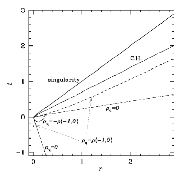
(a) Lines of $\rho_{\mbox{q}}=\mbox{const}$

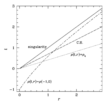
(b) Lines of $\rho=\mbox{const}$ and $\rho_{\mbox{q}}=\rho$

Fig. 16: Plots of (a) lines $\rho_{\mbox{q}}=$ const and (b) $\rho=$ const and $\rho_{\mbox{q}}=\rho$ in the self-similar LTB spacetime. Solid, long-dashed-dotted, dashed, dashed-dotted, long-dashed, long-dashed-short-dashed and dotted lines denote singularity, Cauchy horizon, $\rho_{\mbox{q}}=\rho(-1,0)$, $\rho_{\mbox{q}}=0$, $\rho_{\mbox{q}}=-\rho(-1,0)$, $\rho=\rho(-1,0)$ and $\rho_{\mbox{q}}=\rho$, respectively.

Next we consider the energy flux measured by the comoving observer. For this observer, the energy flux becomes

$$F_{\mbox{q}}\equiv\langle T_{\mu\nu}\rangle u^{\mu}n^{\nu}=\frac{\langle T_{UU}\rangle}{r^{2}(z-R_{,r})^{2}}-\frac{\langle T_{VV}\rangle}{r^{2}(z+R_{,r})^{2}}.$$ (3.136)

In the interior region, outgoing part of flux is proportional to $\langle T_{UU}\rangle$ and ingoing part of flux is proportional to $\langle T_{VV}\rangle$. Here we define the ingoing part $F_{\mbox{in}}$ and the outgoing part $F_{\mbox{out}}$ of the flux as

$$F_{\mbox{in}}\equiv\frac{\langle T_{VV}\rangle}{r^{2}(z+R_{,r})^{2}},~{}~{}~{}~{}~{}F_{\mbox{out}}\equiv\frac{\langle T_{UU}\rangle}{r^{2}(z-R_{,r})^{2}}.$$ (3.137)

Following the sign of these two values we divide the interior region into four parts. Region I: positive ingoing and outgoing parts, region II: negative outgoing and positive ingoing parts, region III: negative ingoing and outgoing parts, and region IV: positive outgoing and negative ingoing parts. The results are shown in Fig. 17. Flux observed by a time-like observer may become zero in region I and III. In fact, the observed flux vanishes at $r=0$ and on the dotted dashed line in Fig. 17.

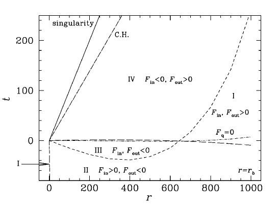
Fig. 17: Signs of ingoing and outgoing parts of flux in the self-similar LTB spacetime. The solid and long-dashed-dotted lines correspond to the singularity and the Cauchy horizon, respectively. The dashed line denotes the line on which the ingoing part of flux vanishes. On the long dashed lines the outgoing part vanishes. Regions I, II, III, and IV correspond to positive ingoing and outgoing parts, positive ingoing and negative outgoing parts, negative ingoing and outgoing parts, and negative ingoing and positive outgoing parts, respectively. On the short-dashed-dotted line, the observed net flux vanishes.

We show this flux schematically in Fig. 18(a). The intensity is proportional to the length of arrows along the $r$-axis. The comoving observers receive inward flux first and then outward flux after the crossing of the line (c). The intensity grows as the Cauchy horizon is approached.

(a) Observed flux

(b) Ingoing and outgoing parts of flux

Fig. 18: Schematic figures (a) for the flux observed by comoving observer and (b) for the ingoing and outgoing parts of flux in the self-similar LTB spacetime. Lines (a) and (b) correspond to the singularity and the Cauchy horizon, respectively. Line (c) denotes the line on which the observed flux vanishes. Regions I, II, III, and IV are similar to those in Fig. 17.

In Fig. 18(b), we show ingoing and outgoing parts of the flux schematically. The intensity is proportional to the length of arrow along the $r$-axis. The future and past directed arrows correspond to the positive and negative flux respectively. The outgoing part has large intensity near the Cauchy horizon. The ingoing part has large intensity only near the central singularity.

Here we summarize the behavior of the quantum field in the interior of the star. At first inward flux appears and then the positive energy is concentrated near the center surrounded by a slightly negative energy region. As the collapse proceeds the central positive energy increases and concentrates within a smaller region. At the naked singularity formation the concentrated positive energy is converted to the outgoing positive diverging flux. The left negative energy goes down across the Cauchy horizon. It will be reach the space-like singularity.

Next we consider the totally radiated energy received at infinity. The radiated power of quantum flux can be expressed as

$$P=\langle T_{\mu\nu}\rangle u^{\mu}n^{\nu}=\alpha^{\prime 2}F_{U}(\beta^{\prime})+F_{u}(\alpha^{\prime})$$ (3.138)

where $u^{\mu}$ is considered as the velocity of a static observer. We plot this in Fig. 19(a). We reproduce the results of the geometric optics estimates for the four-dimensional model, i.e., the inverse square dependence for the retarded time in an approach to the Cauchy horizon.

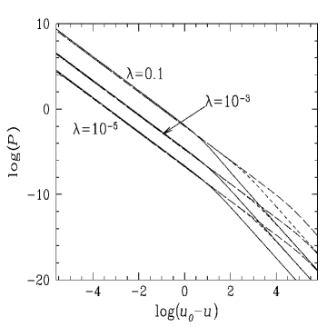
(a) Power

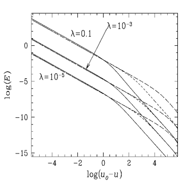
(b) Energy

Fig. 19: (a) Radiated power and (b) integrated energy received at infinity in the self-similar LTB spacetime. Upper, middle and lower lines correspond to $\lambda=0.1$ ,$10^{-3}$ and $10^{-5}$, respectively. Solid, dashed and long-dashed lines correspond to $r_{b}=10$, $10^{3}$ and $10^{5}$, respectively.

The totally radiated energy is obtained from the integration of $P$ with respect to the retarded time at the future null infinity. The results are shown in Fig. 19(b). We see that the totally emitted energy is much smaller than the mass of the original star in the range that the semi-classical approximation can be trusted. We can see that the positive divergence of the radiated power comes from the term $\alpha^{\prime 2}F_{U}(\beta^{\prime})$ which has strong dependence on the spacetime geometry in the interior of the star.

Let us turn to the inspection for the black hole formation. For larger $u$ there appears difference between the naked singularity case and the covered one. This difference mainly depend on the behavior of $\alpha^{\prime}$. In an approach to the event horizon, $w$ goes to unity and then $\alpha^{\prime}$ goes to zero. It is easy to see that only the second term of the radiated power is left in this limit and it becomes

$$F_{u}(\alpha^{\prime})=\frac{1}{192\pi\left(2M\right)^{2}}.$$ (3.139)

This means that $F_{u}(\alpha^{\prime})$ is interpreted as the Hawking radiation contribution. From Eq. (3.39) we obtain

$$\langle T_{vv}\rangle=-\frac{1}{192\pi\left(2M\right)^{2}}$$ (3.140)

at the event horizon. This ingoing negative flux crossing into the black hole is balanced with the energy loss by the positive Hawking flux.

There is similar balance between ingoing and outgoing parts at the Cauchy horizon for the naked singularity explosion. In the asymptotic region positive diverging flux is observed in an approach to the Cauchy horizon. It has been shown above that there is negative ingoing flux crossing the Cauchy horizon. This negative flux diverge only at the central naked singularity. This diverging negative ingoing flux is balanced with the diverging positive outgoing flux which propagates along the Cauchy horizon.

3.4 Naked singularities and quantum gravity

The above discussions are based on quantum field theory in curved spacetime. It may lose its validity if we consider a time interval which is shorter than the Planck time $t_{Planck}$. Therefore, the expressions for the energy radiated from a forming naked singularity can be conceivable at least at $u\mathrel{\mathchoice{\lower 3.0pt\vbox{\halign{$\m@th\displaystyle\hfill#\hfil$\cr<\crcr\sim\crcr}}}{\lower 3.0pt\vbox{\halign{$\m@th\textstyle\hfill#\hfil$\cr<\crcr\sim\crcr}}}{\lower 3.0pt\vbox{\halign{$\m@th\scriptstyle\hfill#\hfil$\cr<\crcr\sim\crcr}}}{\lower 3.0pt\vbox{\halign{$\m@th\scriptscriptstyle\hfill#\hfil$\cr<\crcr\sim\crcr}}}}u_{0}-t_{Planck}$. For self-similar dust collapse, it is easily found that the emitted energy does not exceed the Planck energy $\sim 10^{16}\mbox{erg}$ until this moment. For the analytic dust collapse, the discussion is not so straightforward, but the result is the same. [116]

It is noted that $\omega_{s}$ may exceed the Planck frequency $\omega_{Planck}$ because $\omega_{s}$ is determined by some combination of two macroscopic scales, the free-fall time and the scale of inhomogeneity. Nevertheless, we can find that the totally radiated energy for this late-time radiation cannot exceed the Planck energy before the Planck time. The proof is the following. If $\omega_{s}>\omega_{Planck}$, then it is found that the late-time radiation is only for $u_{0}-u<\omega_{s}^{-1}<t_{Planck}$. Therefore, we only have to consider $\omega_{s}<\omega_{Planck}$. For this case, it is found

$$E_{u_{0}-u\sim t_{Planck}} \sim (\omega_{s}\omega_{Planck})^{1/2}<\omega_{Planck},$$ (3.141)

$$\hat{E}_{u_{0}-u\sim t_{Planck}} \sim \omega_{Planck}\left(\frac{\omega_{s}}{\omega_{Planck}}\ln\frac{\omega_{Planck}}{\omega_{s}}\right)<\omega_{Planck},$$ (3.142)

where the second inequality comes from the fact that the function $-x\ln x$ has a maximum value $e^{-1}$ in the domain $0<x<1$. Therefore, we can conclude that the totally radiated energy of the late-time emission does not exceed the Planck energy.

It follows that the further evolution of the star will depend on quantum gravitational effects, and without invoking quantum gravity it is not possible to say whether the star radiates away on a short time or settles down into a black hole state.

3.5 Discussion

Quantum particle creation during the formation process of naked singularity in dust collapse results in diverging flux emission within a semi-classical theory of quantum fields in curved space. The discussions so far have been based on some specific models of naked singularities. However, calculations are dependent not on the matter fields but on the spacetime geometry around the singularity. Therefore, we can conjecture that the discussions and results will apply to a rather wider class of naked singularities which develop from regular initial data. Although it is not certain whether this phenomenon may be relevant to any observations, several authors have speculated naked singularities as a possible central engine of gamma-ray bursts. [110, 117] Any way, to answer the question may be out of scope of a semi-classical theory of quantum fields in curved space. Apart from the observational aspects, the contribution of emitted quantum particles as a source of gravitational field may become important in more realistic situations. The argument that it may prohibit the formation of naked singularities leads to the quantum version of cosmic censorship conjecture. In particular, the balance relation between positively diverging outgoing flux to infinity and negatively diverging ingoing flux to naked singularity may suggest the quantum version of “naked singularity evaporation conjecture” proposed by Nakamura, Shibata and Nakao. [99]

4 Summary

We have several examples in which naked singularity forms as a result of time development of regular initial Cauchy data, as we have seen in §1. However, we should not conclude that they alone disprove the cosmic censorship conjecture in the exact meaning. In all of these examples, some kind of high symmetries, such as spherical symmetry, axisymmetry, cylindrical symmetry and self-similarity, are assumed. Our knowledge on the effects of deviations from these symmetries on the naked singularities has been quite restricted so far. In critical collapse, it is known that the occurrence of a zero-mass black hole, which is regarded as naked singularity, is realized as a result of the exact fine-tuning. This means that it is a zero-measure event even within the assumed symmetry. In other cases, it is quite difficult in general to answer the question whether the appearance of naked singularity is generic or not. It should be also noted that there is no generally accepted standard measure of the space of initial data sets. Apart from genericity, in some of the examples of naked singularities, matter fields cannot be considered as realistic, such as a dust fluid and null dust. It is also difficult to answer the question what matter model is physically reasonable. Some people consider that elementary fields such as a scalar field will be physically reasonable matter models. However, generally speaking, it is only at the stage in which quantum effects become so important that such field descriptions of matter fields will be useful. Others consider that a system of infinitely many self-gravitating collisionless particles, i.e., the Einstein-Vlasov system will be suitable for the proof or disproof of the cosmic censorship conjecture. This proposition seems to be reasonable from the standing point that singularities that form also in Newtonian gravity should not be taken seriously, because of the global existence theorem of regular solutions with nonsingular initial data sets in the corresponding Newtonian system. However, unfortunately, we do not know any realistic matter field which is expected to behave like the Einstein-Vlasov system in an extremely high-density regime.

However, these examples of naked singularities strongly motivate us to imagine, as a possible stage of gravitational collapse, extremely high-density and/or high-curvature regions uncovered by horizons. In these strongly curved regions, general relativistic effects will become crucial. In fact, it is considered that classical general relativity cannot apply beyond some energy scale, which will be characterized by the Planck scale. Therefore, the existence of classical solutions with naked singularity formed from regular initial data will imply not only the limitation of future predictability of general relativity but also the possibility that new frontier beyond general relativity may be exposed to us. Of course, if a naked singularity is a generic outcome of gravitational collapse, the importance to examine its consequences is much more increased.

If naked singularity is a possible outcome of gravitational collapse, it may provide an exotic source of gravitational wave burst. Gravitational wave generation reflects the dynamical motion of the spacetime in strongly curved regions and they will directly reach us without obstructions unlike electromagnetic waves. As we have seen in §2, for linearized nonspherical perturbations of spherical dust collapse, not the energy flux of gravitational waves but the perturbation of the spacetime curvature blows up unboundedly as one approaches the Cauchy horizon of the background spacetime. This conclusion is also derived semi-analytically using the quadrupole formula for the gravitational wave emission from the dust collapse in Newtonian gravity. From this fact, we may imagine that some sort of perturbations concerning spacetime curvature will be considerably amplified near the Cauchy horizon of a forming naked singularity, although it is not clear if this amplification can be related to any observable of a distant observer. This result also implies weak instability of the Cauchy horizon. Since it means the breakdown of the linearized perturbation scheme, some nonlinear analysis is necessary to make the conclusion clear. As we are having high sensitivity to gravitational waves by laser interferometric gravitational wave detectors, gravitational wave observations will provide interesting information of strongly curved regions.

In addition to classical gravitational radiation, we have seen quantum particle creation from a forming naked singularity in the spherical dust collapse in §3. The calculation of this emission is based on quantum field theory in curved spacetime. The calculation goes parallel to that of the Hawking radiation of black holes. The only difference is the form of the mapping function between the advanced and retarded time coordinates, which comes from the behavior of ingoing and outgoing radial null geodesics in the curved spacetime. The result is that a forming naked singularity emits explosive radiation at the final epoch. This conclusion comes from the fact that the mapping function has only lower differentiability at the Cauchy horizon. It is expected that this property of the mapping function will be common to a wide class of naked singularities. In the case of the two dimensional self-similar dust collapse, the back reaction effects of quantum radiation on the spacetime geometry will be negligible at least until the singularity formation. The radiated positive energy originates from the vacuum energy in the region surrounding the center. A large amount of positive energy is gradually concentrated and accumulated around the center in the course of the singularity formation. After that, the positive energy turns into positive outgoing flux just before the singularity formation. In addition to the back reaction effects, there appears a rather subtle problem between quantum field theory and quantum gravity. If we accept the Planck length a priori as the shortest length scale of quantum field theory, the total amount of radiated energy from a forming naked singularity cannot exceed the Planck energy as long as quantum field theory is justified. Actually, the total amount of radiated energy is greatly dependent on the shortest length scale of quantum field theory.

In conclusion, the cosmic censorship conjecture has provided a strong motivation for researchers in this field. This conjecture was intended to conserve the completeness of future predictability of classical theory. However, we are now convinced of the limitation of classical theory as theory of everything. In this point of view, known examples of naked singularities imply that the future predictability of classical theory is violated in a finite-measure set of initial data sets. Then, we may pay our attention to more general features of gravitational collapse. In fact, classical gravitational wave radiation and quantum particle emission from a forming naked singularity, which have been discussed in this paper, are both irrespective of the final outcome of the forming naked singularity, because these calculations are basically independent of the spacetime geometry in the causal future of the singularity. In this respect, the forming naked singularity can be regarded as an example of inhomogeneously runaway collapsing systems. It could be said that our understanding of gravitational collapse might have been too much based on the spherically symmetric homogeneous collapse, such as the Oppenheimer-Snyder model. Gravitational collapse in more general situations is now and will be an active and attractive field in gravitational physics.

A Gauge-Invariant Perturbations

In this appendix we give a brief introduction to the formalism of Gerlach and Sengupta [91, 92] for perturbations around the most general spherically symmetric spacetime.

We consider a general spherically symmetric spacetime with metric

$$g_{\mu\nu}dx^{\mu}dx^{\nu}\equiv g_{ab}(x^{d})dx^{a}dx^{b}+R^{2}(x^{d})\gamma_{AB}(x^{D})dx^{A}dx^{B}$$ (A.1)

and stress-energy tensor

$$t_{\mu\nu}dx^{\mu}dx^{\nu}\equiv t_{ab}(x^{d})dx^{a}dx^{b}+\frac{1}{2}t_{A}^{~{}A}R^{2}(x^{d})\gamma_{AB}(x^{D})dx^{A}dx^{B},$$ (A.2)

where $\gamma_{AB}dx^{A}dx^{B}=d\theta^{2}+\sin^{2}\theta d\phi^{2}$. Lowercase Latin indices refer to radial and time coordinates, while uppercase Latin indices refer to $\theta$ and $\phi$.

Now we introduce arbitrary perturbations of this spacetime. The angular dependence of perturbations is decomposed into series of tensorial spherical harmonics. The scalar spherical harmonics are $Y_{l}^{m}(x^{A})$. A basis of vector harmonics is formed by $Y_{l~{}:A}^{m}$ and $S_{l~{}A}^{m}\equiv\epsilon_{A}^{~{}B}Y_{l~{}:B}^{m}$. A basis of symmetric rank-two tensor harmonics is formed by $Y_{l}^{m}\gamma_{AB}$, $Z_{l~{}AB}^{m}\equiv Y_{l~{}:AB}^{m}+(l(l+1)/2)Y_{l}^{m}\gamma_{AB}$ and $S_{l~{}A:B}^{m}+S_{l~{}B:A}^{m}$. For $l=0$ and $1$, the last two tensors vanish identically. Linear perturbations with different $l$ and $m$ decouple. In the following, we suppress these indices. We also suppress the explicit summation over them. Perturbations with different values of $m$ for the same $l$ have the same dynamics on a spherically symmetric background, and therefore $m$ does not appear in the field equations. Spherical harmonics are called even parity if they have parity $(-1)^{l}$ under spatial inversion and odd parity if they have parity $(-1)^{l+1}$. Even and odd perturbations decouple.

The odd-parity perturbations are expressed as

$$h_{\mu\nu}dx^{\mu}dx^{\nu}=h_{a}(x^{c})S_{B}(dx^{a}dx^{B}+dx^{B}dx^{a})+h(x^{c})S_{(A:B)}dx^{A}dx^{B}$$ (A.3)

for the metric and

$$\mathchar 28929\relax t_{\mu\nu}dx^{\mu}dx^{\nu}=\mathchar 28929\relax t_{a}(x^{c})S_{A}(dx^{a}dx^{A}+dx^{A}dx^{a})+\mathchar 28929\relax t(x^{c})S_{(A:B)}dx^{A}dx^{B}$$ (A.4)

for matter. The even-parity perturbations are

$$h_{\mu\nu} = h_{ab}(x^{d})Ydx^{a}dx^{b}+h_{a}(x^{d})Y_{:B}(dx^{a}dx^{B}+dx^{B}dx^{a})$$ (A.5)

$$+[K(x^{d})R^{2}\gamma_{AB}Y+G(x^{d})R^{2}Z_{AB}]dx^{A}dx^{B}$$

for the metric and

$$\mathchar 28929\relax t_{\mu\nu} = \mathchar 28929\relax t_{ab}(x^{d})Ydx^{a}dx^{b}+\mathchar 28929\relax t_{a}(x^{d})Y_{:B}(dx^{a}dx^{B}+dx^{B}dx^{a})$$ (A.6)

$$+[\mathchar 28929\relax t^{3}(x^{d})R^{2}\gamma_{AB}Y+\mathchar 28929\relax t^{2}(x^{d})R^{2}Z_{AB}]dx^{A}dx^{B}$$

for matter. Here covariant derivatives are distinguished as follows:

$$\gamma_{AB:C}\equiv 0,~{}~{}~{}~{}~{}g_{ab|c}\equiv 0.$$ (A.7)

For convenience, we introduce

$$v_{a}\equiv\frac{R_{,a}}{R},$$ (A.8)

and

$$p_{a}\equiv h_{a}-\frac{1}{2}R^{2}G_{,a}.$$ (A.9)

We then introduce gauge-invariant variables to eliminate gauge ambiguities in perturbations. The gauge transformation is induced by the infinitesimal vector fields

$$\xi_{\mu}dx^{\mu}=M(x^{c})S_{A}dx^{A},$$ (A.10)

for odd parity and

$$\xi_{\mu}dx^{\mu}=\xi_{a}(x^{c})Ydx^{a}+\xi(x^{c})Y_{:A}dx^{A}$$ (A.11)

for even parity. The odd-parity gauge-invariant metric variables are given by

$$k_{a}\equiv h_{a}-\frac{1}{2}R^{2}\partial_{a}\left(\frac{h}{R^{2}}\right).$$ (A.12)

The odd-parity gauge-invariant matter variables are given by the combinations

$$L_{a} \equiv t_{a}-\frac{1}{2}\bar{T}_{B}^{~{}B}h_{a},$$ (A.13)

$$L \equiv t-\frac{1}{2}\bar{T}_{B}^{~{}B}h.$$ (A.14)

A set of even-parity gauge-invariant metric perturbations is defined as

$$k_{ab} \equiv h_{ab}-(p_{a|b}+p_{b|a}),$$ (A.15)

$$k \equiv K+\frac{l(l+1)}{2}G-2v^{a}p_{a}.$$ (A.16)

A set of even-parity gauge-invariant matter perturbations is defined as

$$T_{ab} \equiv \mathchar 28929\relax t_{ab}-t_{ab|c}p^{c}-t_{a}^{~{}c}p_{c|b}-t_{b}^{~{}c}p_{c|a},$$ (A.17)

$$T_{a} \equiv \mathchar 28929\relax t_{a}-t_{a}^{~{}c}p_{c}-R^{2}(t_{A}^{~{}A}/4)G_{,a},$$ (A.18)

$$T^{3} \equiv \mathchar 28929\relax t^{3}-(p^{c}/R^{2})(R^{2}t_{A}^{~{}A}/2)_{,c}+l(l+1)(t_{A}^{~{}A}/4)G,$$ (A.19)

$$T^{2} \equiv \mathchar 28929\relax t^{2}-(R^{2}t_{A}^{~{}A}/2)G.$$ (A.20)

The linearized Einstein equations, expressed only in terms of gauge-invariant perturbations, are

$$k^{a}_{~{}|a} = 16\pi L,~{}~{}~{}~{}~{}~{}(l\geq 2)$$ (A.21)

$$-\left[R^{4}\left(\frac{k_{a}}{R^{2}}\right)_{|c}-R^{4}\left(\frac{k_{c}}{R^{2}}\right)_{|a}\right]^{|c}+(l-1)(l+2)k_{a} = 16\pi R^{2}L_{a},~{}~{}(l\geq 1)$$ (A.22)

for odd parity and

$$2v^{c}\left(k_{ab|c}-k_{ca|b}-k_{cb|a}\right)-\left[\frac{l(l+1)}{R^{2}}+G_{c}^{~{}c}+G_{A}^{~{}A}+2\cal{R}\right]k_{ab}$$

$$-2g_{ab}v^{c}\left(k_{ed|c}-k_{ce|d}-k_{cd|e}\right)g^{ed}+g_{ab}\left(2v^{c|d}+4v^{c}v^{d}-G^{cd}\right)k_{cd}$$

$$+g_{ab}\left[\frac{l(l+1)}{R^{2}}+\frac{1}{2}\left(G_{c}^{~{}c}+G_{A}^{~{}A}\right)+\cal{R}\right]k_{d}^{~{}d}+2\left(v_{a}k_{,b}+v_{b}k_{,a}+k_{,a|b}\right)$$

$$-g_{ab}\left[2{k_{,c}}^{|c}+6c^{c}k_{,c}-\frac{(l-1)(l+2)}{R^{2}}k\right]=-16\pi T_{ab},$$ (A.23)

$$k_{,a}-{k_{ac}}^{|c}+{{k_{c}}^{c}}_{|a}-v_{a}k_{c}^{~{}c} = -16\pi T_{a},$$ (A.24)

$$-\left({k_{,c}}^{|c}+2v^{c}k_{,c}+G_{A}^{~{}A}k\right)+\left[{k_{cd}}^{|c|d}+2v^{c}{k_{cd}}^{|d}+2(v^{c|d}+v^{c}v^{d})k_{cd}\right]$$

$$-g_{ab}\left[{{{k_{c}}^{c}}_{|d}}^{|d}+v^{c}{{k_{d}}^{d}}_{|c}+{\cal{R}}k_{c}^{~{}c}-\frac{l(l+1)}{R^{2}}k\right]=-16\pi T^{3},$$ (A.25)

$$k_{c}^{~{}c} = -16\pi T^{2}$$ (A.26)

for even parity, where $\cal{R}$ is the Gaussian curvature of the 2-dimensional submanifold $M^{2}$ spanned by $x^{a}$, and

$$G_{ab} \equiv -2\left(v_{a|b}+v_{a}v_{b}\right)+g_{ab}\left(2v_{a}^{~{}|a}+3v_{a}v^{a}-\frac{1}{R^{2}}\right),$$ (A.27)

$$G_{A}^{~{}A} \equiv 2\left(v_{a}^{~{}|a}+v_{a}v^{a}-{\cal{R}}\right).$$ (A.28)

The linearized conservation equation [$\delta(T^{\mu\nu}_{~{}~{};\nu})=0$] reduces to

$$\left(R^{2}L^{a}\right)_{|a}=\left(l-1\right)\left(l+2\right)L,~{}~{}~{}~{}~{}~{}~{}~{}~{}(l\geq 1)$$ (A.29)

for odd parity and

$$\frac{\left(R^{2}T^{a}\right)_{|a}}{R^{2}}+T^{3}-\frac{\left(l-1\right)\left(l+2\right)}{2R^{2}}T^{2} = \frac{1}{2}t_{A}^{~{}A}\left(k-\frac{1}{2}k_{c}^{~{}c}\right)+\frac{1}{2}t^{ab}k_{ab},$$ (A.30)

$$\frac{\left(R^{2}T_{ab}\right)^{|b}}{R^{2}}-\frac{T_{a}l\left(l+1\right)}{R^{2}}-2v_{a}T^{3} = \frac{1}{2}k_{bc|a}t^{bc}+k_{cb}^{|b}t^{c}_{~{}a}-\frac{1}{2}k_{c~{}|b}^{~{}c}t^{b}_{~{}a}$$ (A.31)

$$-k_{,c}t^{c}_{~{}a}+\frac{1}{2}\left(k_{,a}-kv_{a}\right)t_{A}^{~{}A}$$

$$+2v^{b}k_{bc}t^{c}_{~{}a}+k^{b}_{~{}c}t^{c}_{~{}a|b}$$

for even parity.

B Power of Gravitational Radiation

In this appendix we examine the asymptotic behavior of the gauge-invariant variables in asymptotically flat spacetime with an outgoing wave condition. Then we can calculate the radiated power of the gravitational waves and thereby grasp the physical meaning of the gauge-invariant quantities.

Note that in vacuum at large distance, the spherically symmetric background metric is identical to the Schwarzschild solution, which is the following (adopting the Schwarzschild coordinates):

$$ds^{2}=-\left(1-\frac{2M}{R}\right)d\tau^{2}+\left(1-\frac{2M}{R}\right)^{-1}dR^{2}+R^{2}\left(d\theta^{2}+\sin^{2}\theta d\phi^{2}\right).$$ (B.1)

To relate the perturbation of the metric to the radiated gravitational power, it is useful to specialize the gauge to the radiation gauge, in which the tetrad components $h_{(\theta)(\theta)}-h_{(\phi)(\phi)}$ and $h_{(\theta)(\phi)}$ fall off as $O(1/R)$, and all other tetrad components fall off as $O(1/R^{2})$ or faster with respect to the following background tetrad basis:

$$e^{a}_{(\tau)} = \left(1-\frac{2M}{R}\right)^{1/2}(d\tau)^{a},$$ (B.2)

$$e^{a}_{(R)} = \left(1-\frac{2M}{R}\right)^{-1/2}(dR)^{a},$$ (B.3)

$$e^{a}_{(\theta)} = R(d\theta)^{a},$$ (B.4)

$$e^{a}_{(\phi)} = R\sin\theta(d\phi)^{a}.$$ (B.5)

In this radiation gauge, the metric perturbations in Eqs. (A.3) and (A.5) behave as

$$h_{0},h_{1} = O\left(\frac{1}{R}\right),$$ (B.6)

$$h_{2} = w(\tau-R_{*})+O(1)$$ (B.7)

for odd parity and as

$$h_{ab} = O\left(\frac{1}{R^{2}}\right),$$ (B.8)

$$h_{a} = O\left(\frac{1}{R}\right),$$ (B.9)

$$K = O\left(\frac{1}{R^{2}}\right),$$ (B.10)

$$G = \frac{g(\tau-R_{*})}{R}+O\left(\frac{1}{R^{2}}\right)$$ (B.11)

for even parity, where

$$R_{*}=R+2M\ln\left(\frac{R}{2M}-1\right)+\mbox{const},$$ (B.12)

and the outgoing wave condition is satisfied. Then, the gauge-invariant metric perturbations (A.15) and (A.16) are calculated as

$$k_{0} = -\frac{1}{2}w^{(1)}R+O(1),$$ (B.13)

$$k_{1} = \frac{1}{2}w^{(1)}R+O(1)$$ (B.14)

for odd parity and

$$k_{\tau\tau} = g^{(2)}R+O(1),$$ (B.15)

$$k_{\tau R} = -g^{(2)}R+O(1),$$ (B.16)

$$k_{RR} = g^{(2)}R+O(1),$$ (B.17)

$$k = -g^{(1)}+O\left(\frac{1}{R}\right)$$ (B.18)

for even parity, where $w^{(n)}$ and $g^{(n)}$ denotes the $n$-th derivatives of $w$ and $g$, respectively.

In this radiation gauge, the radiated power $P$ per solid angle is given by the formula derived by Landau and Lifshitz [118] from their stress-energy pseudo-tensor:

$$\frac{dP}{d\mathchar 28938\relax}=\frac{R^{2}}{16\pi}\left[\left(\frac{\partial h_{(\theta)(\phi)}}{\partial\tau}\right)^{2}+\frac{1}{4}\left(\frac{\partial h_{(\theta)(\theta)}}{\partial\tau}-\frac{\partial h_{(\phi)(\phi)}}{\partial\tau}\right)^{2}\right].$$ (B.19)

For the axisymmetric mode, (i.e. $m=0$), the above formula is reduced to

$$\frac{dP}{d\mathchar 28938\relax}=\frac{1}{64\pi}(w^{(1)})^{2}A_{l}(\theta)$$ (B.20)

for odd parity and

$$\frac{dP}{d\mathchar 28938\relax}=\frac{1}{64\pi}(g^{(1)})^{2}A_{l}(\theta)$$ (B.21)

for even parity, where

$$A_{l}(\theta)\equiv\frac{2l+1}{4\pi}\sin^{4}\theta\left(\frac{d^{2}P_{l}(\cos\theta)}{(d\cos\theta)^{2}}\right)^{2}.$$ (B.22)

It is found that for the monopole and dipole modes, the radiated power exactly vanishes. By using gauge-invariant quantities and integrating over the $4\pi$ solid angle, the formula for the power of the gravitational radiation for $l\geq 2$ is obtained as

$$\frac{dP}{d\mathchar 28938\relax} = \frac{1}{16\pi}\frac{k_{0}^{2}}{R^{2}}A_{l}(\theta)=\frac{1}{16\pi}\frac{k_{1}^{2}}{R^{2}}A_{l}(\theta),$$ (B.23)

$$P = \frac{1}{16\pi}B_{l}\frac{k_{0}^{2}}{R^{2}}=\frac{1}{16\pi}B_{l}\frac{k_{1}^{2}}{R^{2}}$$ (B.24)

for odd parity and

$$\frac{dP}{d\mathchar 28938\relax} = \frac{1}{64\pi}k^{2}A_{l}(\theta),$$ (B.25)

$$P = \frac{1}{64\pi}B_{l}k^{2}$$ (B.26)

for even parity, where

$$B_{l}\equiv\frac{(l+2)!}{(l-2)!}.$$ (B.27)

C Equations for Even-Parity Perturbations

For marginally bound LTB spacetime linearized quadrupole Einstein equations are

$$\frac{4}{R^{2}}q+\frac{1}{RR^{\prime}}q^{\prime}+\frac{\dot{R}}{R}\dot{q}$$

$$\quad-\frac{6}{R^{2}}{k}+\left(\frac{2}{RR^{\prime}}-\frac{R^{\prime\prime}}{R^{\prime 3}}\right)k^{\prime}-\left(2\frac{\dot{R}}{R}+\frac{\dot{R^{\prime}}}{R^{\prime}}\right)\dot{k}+\frac{1}{R^{\prime 2}}k^{\prime\prime}$$

$$\quad+2\left(\frac{\dot{R}}{R^{2}R^{\prime}}-\frac{\dot{R}R^{\prime\prime}}{RR^{\prime 3}}+\frac{\dot{R^{\prime}}}{RR^{\prime 2}}\right){k_{01}}+2\frac{\dot{R}}{RR^{\prime 2}}{k_{01}}^{\prime}=-8\pi\delta\rho,$$ (C.1)

$$-\frac{\dot{R}}{R}q^{\prime}+\frac{R^{\prime}}{R}\dot{q}+\left(2\frac{\dot{R}}{R}-\frac{\dot{R^{\prime}}}{R^{\prime}}\right)k^{\prime}+\dot{k^{\prime}}-\frac{3}{R^{2}}{k_{01}} = -8\pi\bar{\rho}V_{1},$$ (C.2)

$$2\frac{R^{\prime 2}}{R^{2}}q-\frac{R^{\prime}}{R}q^{\prime}-\frac{R^{\prime 2}\dot{R}}{R}\dot{q}+4\frac{R^{\prime 2}\dot{R}}{R}\dot{k}+R^{\prime 2}\ddot{k}$$

$$\quad-2\frac{R^{\prime}\dot{R}}{R^{2}}{k_{01}}-2\frac{R^{\prime}}{R}\dot{k_{01}}=0,$$ (C.3)

$$-2\frac{\dot{R^{\prime}}}{R^{\prime}}q-\dot{q}+2\frac{\dot{R^{\prime}}}{R^{\prime}}{k}+2\dot{k}+\frac{R^{\prime\prime}}{{R^{\prime}}^{3}}{k_{01}}-\frac{1}{R^{\prime 2}}{k_{01}}^{\prime} = -16\pi\bar{\rho}V_{2},$$ (C.4)

$$q^{\prime}+\dot{k_{01}}+\frac{\dot{R^{\prime}}}{R^{\prime}}{k_{01}} = 0,$$ (C.5)

$$\left(\frac{R^{2}R^{\prime\prime}}{R^{\prime 3}}-2\frac{R}{R^{\prime}}\right)q^{\prime}-\left(2R\dot{R}+3\frac{R^{2}\dot{R^{\prime}}}{R^{\prime}}\right)\dot{q}-\frac{R^{2}}{R^{\prime 2}}q^{\prime\prime}-R^{2}\ddot{q}$$

$$\quad+4\left(R\dot{R}+\frac{R^{2}\dot{R^{\prime}}}{R^{\prime}}\right)\dot{k}+2R^{2}\ddot{k}+2\left(\frac{RR^{\prime\prime}\dot{R}}{R^{\prime 3}}-\frac{R\dot{R^{\prime}}}{R^{\prime 2}}\right)k_{01}$$

$$\quad-2\frac{R\dot{R}}{R^{\prime 2}}{k_{01}}^{\prime}+2\left(\frac{R^{2}R^{\prime\prime}}{R^{\prime 3}}-\frac{R}{R^{\prime}}\right)\dot{k_{01}}-2\frac{R^{2}}{R^{\prime 2}}\dot{k_{01}^{\prime}}=0,$$ (C.6)

$$-k_{00}+\frac{1}{R^{\prime 2}}k_{11} = 0.$$ (C.7)

Here we can use Eq. (C.7) to eliminate $k_{11}$ in Eqs. (C)–(C).

D Characteristic Frequency of a Naked Singularity

In §1.2.2, we set the initial data at $t=0$ and specified the solution. At an arbitrary time $t<t_{0}$, we can expand the mass function $F(r)$ in terms of the circumferential radius $R$ for marginally bound collapse with an analytic initial density profile as

$$F(r)=F_{3}\left(\frac{t_{0}-t}{t_{0}}\right)^{-2}R^{3}+F_{5}\left(\frac{t_{0}-t}{t_{0}}\right)^{-13/3}R^{5}+\cdots.$$ (D.1)

Although the quantities $F(r)$, $(t_{0}-t)$ and $R$ have physical meanings, $t_{0}$ itself has no physical meaning, because it explicitly depends on the choice of the origin of the time coordinate $t$. This implies that neither $F_{3}$ nor $F_{5}$, but, rather, the combination $F_{3}^{13}/F_{5}^{6}$ characterizes the time evolution of the density profile in the neighborhood of the center, because the dependence on $t_{0}$ vanishes only through this combination of $F_{3}$ and $F_{5}$.

Observing that the free-fall time and the scale of the inhomogeneity at the time $t=0$ are

$$t_{0} \equiv \frac{2}{3}F_{3}^{-1/2},$$ (D.2)

$$l_{0} \equiv \left(\frac{-F_{5}}{F_{3}}\right)^{-1/2},$$ (D.3)

we can easily find that the following constant, which has the dimension of frequency, characterizes naked singularity formation in the LTB spacetime:

$$\omega_{s}\equiv\frac{l_{0}^{6}}{t_{0}^{7}}.$$ (D.4)

References

- [1] R. Penrose, Phys. Rev. Lett. 14 (1965), 57.
- [2] S. W. Hawking, Proc. Roy. Soc. London A 300 (1967), 187.
- [3] S. W. Hawking and R. Penrose, Proc. Roy. Soc. London A 314 (1970), 529.
- [4] R. Penrose, Riv. Nuovo Cim. 1 (1969), 252.
- [5] R. Penrose, in General Relativity, an Einstein Centenary Survey, ed. S.W. Hawking and W. Israel (Cambridge University Press, Cambridge, England, 1979), p. 581.
- [6] R. Casadio and B. Harms, hep-th/0110255.
- [7] S. W. Hawking and G.F.R. Ellis, The large scale structure of space-time (Cambridge University Press, Cambridge, England, 1973).
- [8] C. W. Misner and D.H. Sharp, Phys. Rev. 136 (1964), 571.
- [9] F. J. Tipler, Phys. Lett. A 64 (1977), 8.
- [10] A. Królak, J. Math. Phys. 28 (1987), 138.
- [11] C. J. S. Clarke, The Analysis of Space-Time Singularities (Cambridge University Press, Cambridge, England, 1993).
- [12] G. Lemaître, Ann. Soc. Sci. Bruxelles I A 53 (1933), 51.
- [13] R. C. Tolman, Proc. Nat. Acad. Sci. 20 (1934), 169.
- [14] H. Bondi, Mon. Not. R. Astron. Soc. 107 (1947), 410.
- [15] P. Yodzis, H.-J. Seifert and H. Müller zum Hagen, Commun. Math. Phys. 34 (1973), 135.
- [16] P. S. Joshi and I. H. Dwivedi, Phys. Rev. D 45 (1993), 5357.
- [17] D. M. Eardley and L. Smarr, Phys. Rev. D 19 (1979), 2239.
- [18] D. Christodoulou, Commun. Math. Phys. 93 (1984), 171.
- [19] T. P. Singh and P. S. Joshi, Class. Quantum Grav. 13 (1996), 559.
- [20] S. Jhingan and P. S. Joshi, Annals of Israel Physical Society Vol. 13 (1997), 357.
- [21] R. P. A. C. Newman, Class. Quantum Grav. 3 (1986), 527.
- [22] S. S. Deshingkar, P. S. Joshi and I. H. Dwivedi, Phys. Rev. D 59 (1999), 044018.
- [23] I. H. Dwivedi, Phys. Rev. D 58 (1998), 064004.
- [24] F. Mena and B. Nolan, Class. Quantum Grav. 18 (2001), 4531.
- [25] S. S. Deshingkar, P. S. Joshi and I. H. Dwivedi, gr-qc/0111053.
- [26] J. R. Oppenheimer and H. Snyder, Phys. Rev. 56 (1939), 455.
- [27] H. Müller zum Hagen, P. Yodzis and H. -J. Seifert, Commun. Math. Phys. 37 (1974), 29.
- [28] A. Ori and T. Piran, Phys. Rev. Lett. 59 (1987), 2137.
- [29] A. Ori and T. Piran, Gen. Relat. Gravit. 20 (1988), 7.
- [30] A. Ori and T. Piran, Phys. Rev. D 42 (1990), 1068.
- [31] T. Foglizzo and R. N. Henriksen, Phys. Rev. D 48 (1993), 4645.
- [32] B. Waugh and K. Lake, Phys. Rev. D 38 (1988), 1315.
- [33] B. Waugh and K. Lake, Phys. Rev. D 40 (1989), 2137.
- [34] T. Harada, Phys. Rev. D 58 (1998), 104015.
- [35] T. Harada and H. Maeda, Phys. Rev. D 63 (2001), 084022.
- [36] T. Harada, Class. Quantum Grav. 18 (2001), 4549.
- [37] B. J. Carr, gr-qc/0003009.
- [38] B. J. Carr and A. A. Coley, Class. Quantum Grav. 16 (1999), R31.
- [39] M. W. Choptuik, Phys. Rev. Lett. 70 (1993), 9.
- [40] A. M. Abrahams and C. R. Evans, Phys. Rev. Lett. 70 (1993), 2980.
- [41] C. R. Evans and J. S. Coleman, Phys. Rev. Lett. 72 (1994), 1782.
- [42] D. W. Neilsen and M. W. Choptuik, Class. Quantum Grav. 17 (2000), 733.
- [43] D. W. Neilsen and M. W. Choptuik, Class. Quantum Grav. 17 (2000), 761.
- [44] T. Koike, T. Hara and S. Adachi, Phys. Rev. Lett. 74 (1995), 5170.
- [45] H. Maeda and T. Harada, Phys. Rev. D 64 (2001), 124024.
- [46] C. Gundlach, Liv. Rev. Rel. 2 (1999), 4.
- [47] D. Christodoulou, Commun. Math. Phys. 109 (1987), 613.
- [48] D. Christodoulou, Commun. Pure Appl. Math. 44 (1991), 339.
- [49] D. Christodoulou, Commun. Pure Appl. Math. 46 (1993), 1131.
- [50] D. Christodoulou, Ann. of Math. 140 (1997), 607.
- [51] D. Christodoulou, Ann. of Math. 149 (1999), 187.
- [52] A. Einstein, Preuss. Akad. Wiss. Berlin Sitzber. (1915), 844.
- [53] B. K. Datta, Gen. Relat. Gravit. 1 (1970), 19.
- [54] H. Bondi, Gen. Relat. Gravit. 2 (1971), 321.
- [55] A. B. Evans, Gen. Relat. Gravit. 8 (1976), 155.
- [56] G. Magli, Class. Quantum Grav. 14 (1997), 1937.
- [57] G. Magli, Class. Quantum Grav. 15 (1998), 3215.
- [58] T. Harada, K. Nakao and H. Iguchi, Class. Quantum Grav. 16 (1999), 2785.
- [59] T. Harada, H. Iguchi and K. Nakao, Phys. Rev. D 58 (1998), 041502.
- [60] S. Jhingan and G. Magli, Phys. Rev. D 61 (2000), 124006.
- [61] H. Kudoh, T. Harada and H. Iguchi, Phys. Rev. D 62 (2000), 104016.
- [62] A. D. Rendall, Liv. Rev. Rel. 3 (2000), 1.
- [63] K. Pfaffelmoser, J. Diff. Eq. 95 (1992), 281.
- [64] A. D. Rendall, in Approaches to Numerical Relativity, ed. R.A. d’Inverno (Cambridge University Press, Cambridge, England, 1992), p. 94.
- [65] G. Rein and A. D. Rendall, Commun. Math. Phys. 150 (1992), 561.
- [66] G. Rein, A. D. Rendall and J. Schaeffer, Commun. Math. Phys. 168 (1995), 467.
- [67] P. C. Vaidya, Current Science 13 (1943), 183.
- [68] P. C. Vaidya, Phys. Rev. 47 (1951), 10.
- [69] P. C. Vaidya, Proc. Indian Acad. Sci. A 33 (1951), 264.
- [70] P. S. Joshi and I. H. Dwivedi, Commun. Math. Phys. 146 (1992), 333.
- [71] P. Szekeres, Phys. Rev. D 12 (1975), 2941.
- [72] P. S. Joshi and A. Królak, Class. Quantum Grav. 13 (1996), 3069.
- [73] S. S. Deshingkar, S. Jhingan and P. S. Joshi, Gen. Relat. Grav. 30 (1998), 1477.
- [74] S. Chandrasekhar and J. B. Hartle, Proc. R. Soc. London A 384 (1982), 301.
- [75] E. Poisson and W. Israel, Phys. Rev. D 41 (1990), 1796.
- [76] P. R. Brady and E. Poisson, Class. Quantum Grav. 9 (1992), 121.
- [77] P. R. Brady, I. G. Moss and R. C. Myers, Phys. Rev. Lett. 80 (1998), 3432.
- [78] S. Hod and T. Piran, Phys. Rev. Lett. 81 (1998), 1554.
- [79] A. Ori, Phys. Rev. D 58 (1998), 084016.
- [80] A. Ori, Phys. Rev. Lett. 83 (1999), 5423.
- [81] K. S. Thorne, in Magic Without Magic, ed. J.R. Klauder (Freeman, San Francisco, USA, 1972), p 231.
- [82] T. Nakamura and H. Sato, Prog. Theor. Phys. 67 (1982), 1396.
- [83] T. Nakamura, K. Maeda, S. Miyama and M. Sasaki, in Proceedings of the 2nd Marcel Grossmann Meeting on General Relativity, ed. R. Ruffini (North-Holand, Amsterdam, Netherland, 1982), p. 675.
- [84] S. L. Shapiro and S. A. Teukolsky, Phys. Rev. Lett. 66 (1991), 994.
- [85] S. L. Shapiro and S. A. Teukolsky, Phys. Rev. D 45 (1992), 2006.
- [86] R. M. Wald and V. Iyer , Phys. Rev. D 44 (1991), R3719.
- [87] C. Barrabes, W. Israel and P. S. Letelier, Phys. Lett. A 160 (1991), 41.
- [88] M. A. Pelath, K. P. Tod and R. M. Wald, Class. Quantum Grav. 15 (1998), 3917.
- [89] H. Iguchi, K. Nakao and T. Harada, Phys. Rev. D 57 (1998), 7262.
- [90] H. Iguchi, T. Harada and K. Nakao, Prog. Theor. Phys. 101 (1999), 1235.
- [91] U. H. Gerlach and U. K. Sengupta, Phys. Rev. D 19 (1979), 2268.
- [92] U. H. Gerlach and U. K. Sengupta, Phys. Rev. D 22 (1980), 1300.
- [93] J. M. Bardeen and T. Piran, Phys. Rep. 96 (1983), 205.
- [94] S. Chandrasekhar and S. Detweiler, Proc. R. Soc. London 344 (1975), 441.
- [95] C. T. Cunningham, R. H. Price and V. Moncrief, Astrophys. J. 224 (1978), 643.
- [96] C. T. Cunningham, R. H. Price and V. Moncrief, Astrophys. J. 230 (1979), 870.
- [97] C. T. Cunningham, R. H. Price and V. Moncrief, Astrophys. J. 236 (1980), 674.
- [98] H. Iguchi, T. Harada and K. Nakao, Prog. Theor. Phys. 103 (2000), 53.
- [99] T. Nakamura, M. Shibata and K. Nakao, Prog. Theor. Phys. 89 (1993), 821.
- [100] K. Nakao, H. Iguchi and T. Harada, Phys. Rev. D 63 (2001), 084003.
- [101] T. A. Apostolatos and K. S. Thorne, Phys. Rev. D 46 (1992), 2435.
- [102] F. Echeverria, Phys. Rev. D 47 (1993), 2271.
- [103] T. Chiba, Prog. Theor. Phys. 95 (1996), 321.
- [104] S. W. Hawking, Commun. Math. Phys. 43 (1975), 199.
- [105] L. H. Ford and L. Parker, Phys. Rev. D 17 (1978), 1485.
- [106] W. A. Hiscock, L. G. Williams and D. M. Eardley, Phys. Rev. D 26 (1982), 751.
- [107] N. D. Birrel and P. C. W. Davies, Quantum Fields in Curved Space (Cambridbe University Press, Cambridge, England, 1982).
- [108] P. C. Davies, S. A. Fulling and W. G. Unruh, Phys. Rev. D 13 (1976), 2720.
- [109] T. Harada, H. Iguchi and K. Nakao, Phys. Rev. D 61 (2000), 101502(R).
- [110] T. Harada, H. Iguchi and K. Nakao, Phys. Rev. D 62 (2000), 084037.
- [111] T. Tanaka and T.P. Singh, Phys. Rev. D 63 (2001), 124021.
- [112] S. Barve, T. P. Singh, C. Vaz and L. Witten, Nucl. Phys. B 532 (1998), 361.
- [113] C. Vaz and L. Witten, Phys. Lett. B 442 (1998), 90.
- [114] S. Barve, T. P. Singh, C. Vaz and L. Witten, Phys. Rev. D 58 (1998), 104018.
- [115] H. Iguchi and T. Harada, Class. Quantum Grav. 18 (2001), 3681.
- [116] T. Harada, H. Iguchi, K. Nakao, T. P. Singh, T. Tanaka, and C. Vaz, Phys. Rev. D 64 (2001), 041501(R).
- [117] P. S. Joshi, N. K. Dadhich and R. Maartens, Mod. Phys. Lett. A 15 (2000), 991.
- [118] L. D. Landau and E. M. Lifshitz, The Classical Theory of Fields (Pergamon, London, England, 1975).