Present address: ]Relativity and Cosmology Group, Department of Mathematics and Applied Mathematics, University of Cape Town, Rondebosch 7701, Cape Town, South Africa

On Scaling Solutions with a Dissipative Fluid

Abstract

We study the asymptotic behaviour of scaling solutions with a dissipative fluid and we show that, contrary to recent claims, the existence of stable accelerating attractor solution which solves the ‘energy’ coincidence problem depends crucially on the chosen equations of state for the thermodynamical variables. We discuss two types of equations of state, one which contradicts this claim, and one which supports it.

Current observational evidence suggests that the Universe is flat and accelerating P (1). Since the average energy-density of matter is relatively low there should consequentially exist a dark energy smoothly distributed with roughly the same magnitude as the matter energy. In general this requires fine-tuning of the initial conditions and has become known as the ‘energy’ coincidence problem. The simplest explanation for this dark energy is a vacuum energy density; however, due to the discrepancy between the “observed” value of the cosmological constant and that predicted by particle physics W (2), alternative mechanisms should be considered. One model that has recently attracted attention explains the “missing” energy in terms of the existence of a minimally coupled scalar field (“quintessence” field) S (3). By a suitable choice of the scalar field interaction potential, the scalar field evolves becoming the dominant contribution to the energy density today. These type of solutions (matter scaling solutions) were first studied in R (4) and their stability, for the exponential potential case, were analyzed in ss (5). However, since FLRW solutions with a perfect fluid and a scalar field evolve towards a scaling solution that does not accelerate (unless matter violates the strong energy condition), Chimento et al. Ch (6) considered a dissipative fluid by means of the existence of a bulk dissipative pressure. Bulk viscosity may be associated with particle production Z (8), may be understood as frictional effects that appears in mixtures U (9) or even to model other kinds of sources (e.g. the string dominated universe described by Turok T (10) or a scalar field Ib (11)).

In Ch (6) the authors studied the effect of the bulk viscosity by using the truncated Israel-Stewart theory I (7) and claimed that there exists a stable attractor that has an accelerated expansion thereby solving the energy coincidence problem. However, their analysis was not complete: the differential equation for the function gamma defined in (10) of their article was not taken into account and the equation of state for the bulk pressure was not stated. In this paper we study the asymptotic behaviour of a FLRW model with a dissipative fluid and a scalar field with exponential potential using two different equations of state for the bulk pressure.

We will show that the claim stated in Ch (6), that there exist stable accelerating matter scaling solutions with non-zero bulk viscosity, cannot be substantiated. We will show that the conclusions in Ch (6) depend crucially on the chosen equation of state for the coefficient of bulk viscosity, $\xi$, and the relaxation time, $\tau$.

We assume a FLRW metric:

$$ds^{2}=-dt^{2}+a^{2}(t)\;d\Omega^{2}$$ (1)

with a source given by a fluid with bulk viscosity and a scalar field with a exponential potential:

$$T_{ab}=T^{\phi}_{ab}+T^{m}_{ab},$$ (2)

where

$$T^{\phi}_{ab}=\phi_{a}\phi_{b}-g_{ab}\left(\frac{1}{2}\phi_{c}\phi^{c}+V(\phi)\right)$$ (3)

and

$$T^{m}_{ab}=\rho u_{a}u_{b}+(p+\sigma)(u_{a}u_{b}+g_{ab}),$$ (4)

where $\sigma$ is the viscous pressure, $p$ is the thermodynamic pressure and $\rho$ is the energy density. Einstein’s equations are then:

$$\dot{H} = -H^{2}-\frac{1}{6}(\rho+3p+3\sigma+2\dot{\phi}^{2}-2V)$$ (5)

$$3H^{2} = \rho+\frac{1}{2}\dot{\phi}^{2}+V-\frac{3K}{a^{2}}\qquad(K=\pm 1,0)$$ (6)

$$\dot{\rho} = -3H(\rho+p+\sigma)$$ (7)

$$\ddot{\phi} = -3H\dot{\phi}-\frac{dV}{d\phi},$$ (8)

where $H\equiv\dot{a}/a$.

The viscous pressure $\sigma$ is assumed to satisfy the truncated Israel-Stewart equation I (7):

$$\sigma+\tau\dot{\sigma}=-3\xi H,$$ (9)

where $\xi$ is the coefficient of bulk viscosity and $\tau$ is the relaxation time ($\xi>0,\tau>0$). Strictly speaking, eq. (9) is valid only when the fluid is close to equilibrium; however, we assume its validity even when the fluid is far from equilibrium. (A more rigourous and comprehensive analysis would utilise the full transport equation of the Israel-Stewart theory.) We will assume a linear barotropic equation of state $p=(\gamma-1)\rho$, where the constant $\gamma$ satisfies $0<\gamma<2$ and two different relations for the coefficient of bulk viscosity and relaxation times.

In the first case we consider the following relations:

$$\qquad\xi=\alpha\rho^{m},\qquad\tau=\frac{\xi}{\rho}=\alpha\rho^{m-1}$$ (10)

which were introduced by Belinskii et al. B (12).

We now introduce a new set of normalized variables:

$$\Omega = \frac{\rho}{3H^{2}},\qquad\Sigma=\frac{\sigma}{H^{2}},\qquad\Psi=\frac{1}{\sqrt{6}}\frac{\dot{\phi}}{H},$$

$$\Gamma = \frac{1}{3}\frac{V}{H^{2}},\qquad h=H^{1-2m},\qquad m\neq\frac{1}{2},$$ (11)

and a new time $\tau$ defined by:

$$H(t)\;dt=d\tau.$$ (12)

The Friedmann equation (6) now becomes:

$$1-\Omega^{2}-\Psi^{2}-\Gamma=-\frac{K}{H^{2}a^{2}},$$ (13)

and Einstein’s equations are now:

$$\Omega^{\prime} = \Omega(-3\gamma+2x)-\Sigma$$ (14)

$$\Sigma^{\prime} = -9\Omega+\Sigma\left[-\frac{1}{\alpha}(3\Omega)^{(1-m)}h+2x\right]$$ (15)

$$\Psi^{\prime} = \Psi(x-3)-\frac{3k}{\sqrt{6}}\Gamma$$ (16)

$$\Gamma^{\prime} = \Gamma(2x+k\sqrt{6}\Psi)$$ (17)

$$h^{\prime} = -(1-2m)hx$$ (18)

where ^′ denotes derivative with respect to $\tau$ and

$$x\equiv 1+\frac{1}{2}(3\gamma-2)\Omega+\frac{1}{2}\Sigma+2\Psi^{2}-\Gamma.$$ (19)

When $m=1/2$ the equation for $H$ decouples from the other equations and the system becomes a four-dimensional system. We will not consider this particular bifurcation situation just yet as it is a special case of the next equation of state considered below.

Before studying the equilibrium points of the above system we present some relevant expressions. The energy density of the scalar field is given by:

$$\rho_{\phi}=\frac{1}{2}\dot{\phi}^{2}+V=3H^{2}(\Psi^{2}+\Gamma)$$ (20)

and

$$\Omega_{\phi}=\frac{\rho_{\phi}}{3H^{2}}=\Psi^{2}+\Gamma.$$ (21)

The adiabatic index of the scalar field is:

$$\gamma_{\phi}\equiv\frac{\rho_{\phi}+p_{\phi}}{\rho_{\phi}}=\frac{\dot{\phi}^{2}}{\frac{1}{2}\dot{\phi}^{2}+V}=\frac{2\Psi^{2}}{\Psi^{2}+\Gamma}.$$ (22)

The deceleration parameter is given by:

$$q=x-1.$$ (23)

We are looking for those equilibrium points that have non vanishing matter and scalar field; i.e., $\Omega\neq 0$, $\Psi\neq 0$ and $\Gamma\neq 0$. From equation (17) one such point corresponds to:

$$x=-k\frac{\sqrt{6}}{2}\Psi.$$ (24)

Equation (18) implies that $h=0$ and therefore $H\rightarrow 0$ when $m<1/2$ and $H\rightarrow\infty$ when $m>1/2$, as the point is approached. From equation (16) we obtain:

$$\Gamma=-\Psi^{2}-\frac{\sqrt{6}}{k}\Psi.$$ (25)

From equation (15) we obtain:

$$0=-9\Omega+2x\Sigma,\qquad\Rightarrow\qquad\Omega=-k\frac{\sqrt{6}}{9}\Psi\Sigma.$$ (26)

Substituting this expression in equation (14) we get:

$$\Psi=\frac{\sqrt{6}}{4k}\left(-\gamma\pm\sqrt{\gamma^{2}+4}\right).$$ (27)

Since $\Gamma>0$, equation (25) implies that $\Psi$ must be negative and therefore only the solution with the minus sign is valid in the above expression. Furthermore, it is easy to see that the condition $\Psi<0$ implies that $\gamma<3/2$. Finally, to obtain $\Sigma$ we substitute equations (24)-(27) into equation (19) and we obtain:

$$\Sigma=-\frac{9}{\sqrt{6}k}\frac{1}{\Psi}\left(1+\frac{\sqrt{6}}{k}\Psi\right).$$ (28)

So the equilibrium point is given by:

$$\Omega = 1-\frac{3}{2k^{2}}\left(\gamma+\sqrt{\gamma^{2}+4}\right)$$

$$\Sigma = \frac{6}{\gamma+\sqrt{\gamma^{2}+4}}\left[1-\frac{3}{2k^{2}}\left(\gamma+\sqrt{\gamma^{2}+4}\right)\right]$$

$$\Psi = -\frac{\sqrt{6}}{4k}\left(\gamma+\sqrt{\gamma^{2}+4}\right)$$

$$\Gamma = \frac{3}{4k^{2}}\left[(2-\gamma)\left(\gamma+\sqrt{\gamma^{2}+4}\right)-2\right]$$

$$h = 0,\qquad\gamma<\frac{3}{2}.$$ (29)

The energy density of the scalar field is

$$\Omega_{\phi}=\Psi^{2}+\Gamma=\frac{3}{2k^{2}}\left(\gamma+\sqrt{\gamma^{2}+4}\right),\qquad\Rightarrow\qquad\Omega+\Omega_{\phi}=1,$$ (30)

and the adiabatic index is

$$\gamma_{\phi}=\frac{2\Psi^{2}}{\Psi^{2}+\Gamma}=\frac{1}{2}\left(\gamma+\sqrt{\gamma^{2}+4}\right)\neq\gamma.$$ (31)

The deceleration parameter in this case is given by:

$$q=\frac{3}{4}(\gamma+\sqrt{\gamma^{2}+4})-1>0.$$ (32)

As in the matter scaling solutions, this equilibrium point represents a flat universe in which the energy density of the scalar field scales with that of the matter; however, in these solutions, the adiabatic indexes are different. More importantly: this solution is not accelerating.

The stability of this equilibrium point is determined by the sign of the eigenvalues of the matrix of the linearized system around the point. After a lengthy calculation one can find that three of the eigenvalues are:

$$3\sqrt{\gamma^{2}+4},\qquad\frac{3}{2}(\gamma+\sqrt{\gamma^{2}+4})-2,\qquad\frac{3}{2}(m-\frac{1}{2})(\gamma+\sqrt{\gamma^{2}+4}).$$ (33)

The sign of the two first eigenvalues are positive whereas the sign of the third depends on the value of $m$. Thus this equilibrium point is not stable. The signs of the two other eigenvalues are difficult to determine.

It is important to note that this is the only equilibrium point with $\Omega\neq 0$, $\Psi\neq 0$ and $\Gamma\neq 0$. If we relax the last condition we obtain, in addition to the former point, a set of equilibrium points corresponding to $\Gamma=0$; i.e., a massless scalar field. From equation (16) we get $x=3$ and from (18) $h=0$. From equations (14) and (15) we obtain:

$$\Sigma=\frac{3}{2}\Omega,\qquad\gamma=\frac{3}{2}.$$ (34)

And finally from equation (19) we obtain:

$$\Omega+\Psi^{2}=1.$$ (35)

In this case $\gamma_{\phi}=2$ and $\Omega_{\phi}=\Psi^{2}$, ($\Omega+\Omega_{\phi}=1$). Again this point is not stable since the eigenvalues of the matrix of the linearised system are:

$$0,\qquad 6(m-\frac{1}{2}),\qquad 6+\sqrt{6}k\Psi,\qquad 4,\qquad 15.$$ (36)

We shall now consider the second case by using the following equations of state:

$$\xi=\xi_{0}\rho^{m}H^{1-2m},~{}~{}~{}\tau=\tau_{0}\rho^{m-r}H^{2r-2m-1},$$ (37)

as used in CvdH (13).

The dynamical system is unchanged except for the evolution equation for the viscous pressure, which now becomes, in terms of the new variables (11)

$$\Sigma^{\prime}=-a\Omega^{r}+\Sigma\left\{-b\Omega^{r-m}+2x\right\}$$ (38)

where

$$a=\frac{3^{1+r}\xi_{0}}{\tau_{0}},~{}~{}~{}{\mathrm{and}}~{}~{}~{}b=\frac{3^{r-m}}{\tau_{0}}$$ (39)

replace our original positive constants $\xi_{0}$ and $\tau_{0}$. As in CvdH (13) we take $r=1$, and we take $m\leq r$ to ensure continuity of (38). Note that as $H$ does not appear in this equation the equation for $h$ decouples from the rest of the dynamical system and we need only study the resulting four-dimensional system. Note also that when $m=1/2$, we have a slight generalisation of the equation of state used above.

There are two equilibrium points which satisfy the requirement $\Omega>0,\Gamma\neq 0,$ and $\Psi\neq 0$. The first has

$$\Sigma = -\Omega\left(k^{2}\left(\Omega-1\right)+3\gamma\right)$$ (40)

$$\Psi = \frac{1}{\sqrt{6}}k\left(\Omega-1\right)$$ (41)

$$\Gamma = \left(\Omega-1\right)\left(\frac{1}{6}k^{2}\left(1-\Omega\right)-1\right),$$ (42)

where $\Omega\in(0,1)$ must satisfy

$$\left(k^{2}\left(\Omega-1\right)+3\gamma\right)\left(b\Omega^{1-m}+k^{2}\left(\Omega-1\right)\right)-a=0$$ (43)

From (42) and $\Gamma>0$ we see that

$$\Omega>1+\frac{6}{k^{2}};$$ (44)

hence, from (43), we see that

$$a<3\left(\gamma+2\right)\left(6+b\Omega^{1-m}\right)$$ (45)

must be satisfied for this point to exist.

The scalar field has density parameter and adiabatic index

$$\Omega_{\phi}=1-\Omega,~{}~{}~{}\gamma_{\phi}=\frac{1}{3}k^{2}\left(1-\Omega\right).$$ (46)

The deceleration parameter is given by

$$q=\frac{1}{2}k^{2}\left(1-\Omega\right)-1=\frac{3}{2}\gamma_{\phi}-1.$$ (47)

This equilibrium point will be stable if all the real parts of the eigenvalues of the Jacobian (of the rhs of the dynamical system) are negative. One of the eigenvalues $\lambda$ is easy to determine:

$$\lambda=k^{2}(1-\Omega)-2=2q;$$ (48)

thus if this point is not inflationary it will not be stable either. The remaining eigenvalues may be determined but the resulting expressions are extremely large. Therefore we will present the results for this point graphically, in figures (1) – (4). As we only wish to qualitatively show the different behaviour which may occur, we only show a few representative cases, and show the variation of behaviour with the parameter $a$. (Recall that $\tau_{0}=3^{1-m}/b$, and $\xi_{0}=a/3^{1+m}b$.) The effect of increasing $b$ may be seen from the figures: for small $b$ (Fig. 1) the upper curve (high density solution) is stable (as $a$ is increased) until $\Omega=1$ is reached at $a\sim 3$ [for $a$ larger than this the high density solution no longer exists; cf. Eq. (45)]; similarly for $b=5$ (Fig. 2), once the upper curve becomes stable (as $a$ is increased) at $a\sim 2$, it remains so until $\Omega=1$, which happens in this case at about $a\sim 14$. For the case $b=10$ (Fig. 3), the higher density solution becomes stable at $a\sim 6$, and $\Omega=1$ is reached at $a\sim 30$. The lower density solution appears never to be stable.

In the figures, we have arbitrarily set $\gamma=1$, $m=0.5$, and $k=2$. The effect of increasing $\gamma$ or $m$ is to push the curves down to lower $\Omega$ (the lower density solution eventually drops off the plots); this does not change the conclusions. Lowering the value of $m$ allows the solution to become stable for smaller $a$ (while pushing the curves up to higher $\Omega$); e.g., in figure (2) with $m=0.1$, the upper curve becomes red (stable) before $a=1$. The effect of changing $k$ is shown in figure (4).

The important point here is that stable solutions exist for a large non-trivial region of the five-dimensional parameter space $\{a,b,m,k,\gamma\}$ of the models.

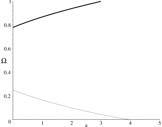
Figure 1: A plot of $\Omega$ versus $a$ for the parameter values $k=2,~{}m=0.5,~{}\gamma=1$ and $b=1$, obtained as the solutions of (43). The thin grey curve (lower) represent solutions which are unstable, while the thicker black curve represents the stable solution, and is thus inflationary, by (48).

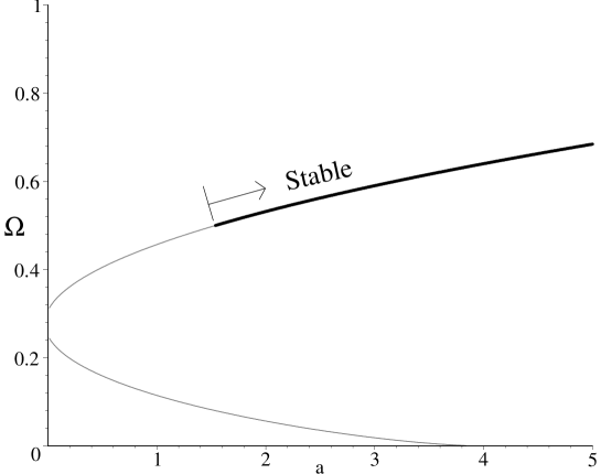
Figure 2: As in figure (1), but now with $b=5$. Again, the thin grey curves represent solutions which are unstable, while the thicker black curve represents the stable solution, and is thus inflationary. This continues increasing with $a$ until $\Omega=1$ is reached when $a\sim 14$ (cf. Figure 3).

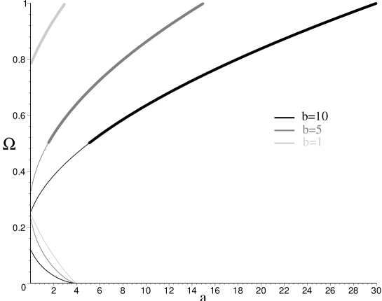
Figure 3: A plot of $\Omega$ versus $a$ for the parameter values $k=2,~{}m=0.5,~{}\gamma=1$ and $b=1,~{}5,~{}10$, obtained as the solutions of (43). This is an amalgamation of the previous two plots, with the additional $b=10$ case represented in black, with the previous cases given in shades of gray, as shown in the key. Again, the thick curves represent the stable solution, and the thinner curves the unstable solutions. The case $b=10$ only becomes stable at high $a$.

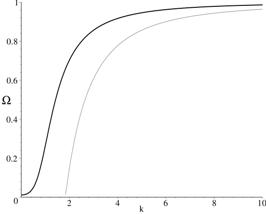
Figure 4: A plot of $\Omega$ versus $k$ for the parameter values $a=1,~{}m=0.6,~{}\gamma=1$ and $b=1$, obtained as the solutions of (43). The effect of increasing $k$ alters the value of $\Omega$, but not the stability; the stable solution (the thick black curve) exists for all $k$, while the unstable solution (thin, grey) becomes available for $k>2$.

The other equilibrium point of interest here is characterised by the following (when $m\neq 1$) :

$$\Omega = \left(\frac{b\left(3\gamma-2\right)}{a+2\left(3\gamma-2\right)}\right)^{\frac{1}{m-1}},$$ (49)

$$\Sigma = -\Omega\left(3\gamma-2\right),$$ (50)

$$\Psi = -\frac{\sqrt{6}}{3k},$$ (51)

$$\Gamma = \frac{4}{3k^{2}}.$$ (52)

For this point

$$\Omega_{\phi}=\frac{2}{k^{2}},~{}~{}~{}\gamma_{\phi}=\frac{2}{3},~{}~{}~{}q=0.$$ (53)

Therefore this point is not inflationary. However, this point in general has non-zero curvature. The stability of this point is difficult to determine analytically, so again we present the results graphically in figure (5). Again we see that there exist stable solutions.

This graph (5) suggests that, for these parameter values, all solutions with $\Omega>0.5$ are unstable, a fact implied by further investigations (although the limiting value of $\Omega$ depends on $k$: indeed for high $k$ there are no unstable solutions). This then suggests that the stability of the solution depends on the curvature: for $\Omega<\Omega_{\phi}=2/k^{2}~{}(=0.5$ in figure (5)) we have the stable solutions, and these have negative curvature, by (13).

Figure 5: A plot of $\Omega$ versus $a$ for the parameter values $k=2,~{}m=0.6,~{}\gamma=1$ (so $\Omega_{\phi}=0.5$); three values for $b$ are represented, $b=5,~{}10,~{}15$, with $b=5$ being the upper curve, and $b=15$ the lower. The thin grey curves represent solutions which are unstable, while the thicker black curves represent the stable solutions.

For the previous two points we have demonstrated the existence of stable solutions; however, we ignored the traditional thermodynamical assumption that the magnitude of the viscosity must be less than the isotropic pressure (we neglected this in the figures by setting $\gamma=1$). However, we note that this does not affect the result. (So, e.g., in the latter equilibrium point this requirement would set $\frac{1}{2}<\gamma<\frac{3}{4}$; stable solutions exist in this case too.)

Finally, if we relax our restriction that $\Gamma\neq 0$, we have another two equilibrium points, given by (when $m\neq 1$)

$$\Omega = \left(\frac{3b(\gamma-2)}{a+18(\gamma-2)}\right)^{\frac{1}{m-1}},$$ (54)

$$\Sigma = 3\Omega(2-\gamma),$$ (55)

$$\Psi^{2} = 1-\Omega=\Omega_{\phi}.$$ (56)

For this point $q=2,$ and $\gamma_{\phi}=2$, so it is not inflationary. Three of the eigenvalues are

$$4,~{}~{}~{}3(2m-1),~{}~{}~{}6+\sqrt{6}k\Psi;$$ (57)

hence this point is not stable.

We have shown that the equations of state play a crucial role in the final evolution of non-perfect fluids with a scalar field. Therefore the claim that a dissipative fluid minimally coupled with a scalar field can resolve the coincidence problem, although suggestive, depends dramatically of the equations of state and on the parameters associated with them.

References

- (1) S.Perlmutter et al., Astrophys. J. 517, 565 (1999).
- (2) S.Weinberg, Rev. Mod. Phys. 61, 1 (1989).
- (3) V.Sahni and A.Starobinsky, Int. J. Mod. Phys. D9, 373 (2000); L.Parker and A.Raval, Phys. Rev. Lett. 86, 749 (2001).
- (4) B.Ratra and P.J.E.Peebles, Phys. Rev. D 37, 3406 (1988).
- (5) E.J.Copeland, A.R.Liddle and D.Wands, Phys. Rev. D 57, 4686 (1998); A.P.Billyard, A.A.Coley and R.J. Van den Hoogen, Phys. Rev. D 58, 123501 (1998).
- (6) L.P.Chimento, A.S.Jakubi and D.Pavón, Phys. Rev. D 62, 063508 (2000).
- (7) W.Israel, Ann. Phys.(N.Y.) 110, 310 (1976); W.Israel and J.Stewart, Ann. Phys.(N.Y.) 118, 341 (1979).
- (8) Ya.B.Zeldovich, Sov. Phys. JETP Lett. 12, 307 (1970).
- (9) N.Udey and W.Israel, Mon. Not. R. Astron. Soc. 199, 1137 (1982).
- (10) N.Turok, Phys. Rev. Lett. 60, 549 (1988).
- (11) A.Di Prisco, L.Herrera and J.Ibáñez, Phys. Rev. D
- (12) V.A.Belinskii, E.S.Nikomarov and I.M.Khalatnikov, Sov. Phy. JETP 50, 213 (1979).
- (13) A.A. Coley and R. van den Hoogen, Class. Quantum Grav. 12, 1977 (1995).