Geometry and topology of singularities in spherical dust collapse

Abstract

We derive some more results on the nature of the singularities arising in the collapse of inhomogeneous dust spheres. (i) It is shown that there are future-pointing radial and non-radial time-like geodesics emerging from the singularity if and only if there are future-pointing radial null geodesics emerging from the singularity. (ii) Limits of various space-time invariants and other useful quantities (relating to Thorne’s point-cigar-barrel-pancake classification and to isotropy/entropy measures) are studied in the approach to the singularity. (iii) The topology of the singularity is studied from the point of view of ideal boundary structure. In each case, the different nature of the visible and censored region of the singularity is emphasized.

I Introduction and summary

The role played by regular initial data in determining the final state of marginally bound spherically symmetric collapse of inhomogeneous dust is well understood. A comprehensive description of this role was first given in sj (1) where explicit necessary and sufficient conditions on the initial data were derived for the existence of a naked singularity. A naked singularity here means a singular region from which there emanates a future-pointing (f.p.) causal geodesic. The result referred to dealt with the existence of f.p. radial null geodesics. Motivated by a desire to (i) study the stability of this result with respect to the introduction of angular momentum and (ii) generalise, in the relevant subsets of the initial data space, to all f.p. causal geodesics, we have studied non-radial null geodesics in spherical dust collapse mn1 (2). We showed that there exist f.p. non-radial null geodesics emanating from the singularity if and only if there exist f.p. radial null geodesics emanating from the singularity. It would be useful to know whether this result can be extended to timelike geodesics in order to give a complete account of all possible causal geodesics. Interesting results in this direction were recently given in desh (3).

The existence of non-radial geodesics outgoing from the singularity might suggest that, topologically, the singularity is not a point. It is therefore interesting to study in more detail the structure of the singularity and in particular to investigate its topological properties. This is a difficult problem since, firstly, the singularity is not part of the space-time and there is no unique definition for the space-time boundary (see seno (4) for a review). Secondly, given the complexity of the geodesic equations, it is difficult to study the topology of a given singular boundary.

In order to have a first intuition about the singularity ‘shape’, we can start by studying the behaviour of the expansion of dust world lines in the neighbourhood of the singularity. In this way, we can classify the singularities as points, cigars, barrels or pancakes dsincosmo (5).

However, this classification says little about topological issues. For example, in a dust filled Friedmann-Lemaitre-Robertson-Walker universe the big bang singularity is point-like in this classification, but is foliated by 2-spheres according to a scheme used below. Furthermore, there are simple examples where this classification scheme does not give any results such as for the singularity in Schwarzschild space-time with negative mass. We recall that in the context of the self-similar collapse of a scalar field, Christodoulou christo-scalar (6) has found an example a singular boundary (see below) which is foliated by points in some sectors and by spheres in other sectors. So, a space-time singularity might not have a distinct unique topology and can possess complicated geometrical features (see also e.g. the Curzon singularity scott (7)). It is therefore of importance to investigate some of these non-trivial issues in the context of spherical dust collapse.

This paper aims to study carefully some aspects of the singularity and its topological properties in Lemaitre-Tolman (LT) space-times. In section II we briefly describe the marginally bound LT model and recall previous results of sj (1) and mn1 (2). In section III, we consider the problem of extending the result of mn1 (2) to all f.p. causal geodesics. In section IV, we investigate the causal structure of the singularity by studying the behaviour of ingoing radial null geodesics. In section V, we shall use Thorne’s classification scheme, which turns out to be of interest in this case beyond merely classifying the singularity. We shall also study the behaviour of a number of space-time invariants in order to investigate the structure of the singularity. These invariants involve the shear and the space-time curvature and have been used e.g. in studies of the Weyl curvature hypothesis penrose (8) as well as in the context of isotropic singularities gw (9). In section VI, we address topological issues by considering non-radial null geodesics emerging from the singularity for self-similar solutions. We end with some conclusions and comments. All our considerations are restricted to the local visibility of the singularity. Another important point to keep in mind is that when dealing with radial geodesics, we will for the most part treat them as curves in the Lorentzian 2-space $\theta=$constant, $\phi=$constant. So a ‘unique’ radial geodesic as referred to in e.g. Proposition 4 is a unique curve in the $r-t$ plane, but is a 2-parameter family of curves in the space-time. The exception is Section VI, where the different angular parameters of radial curves play an essential role. A bullet $\bullet$ indicates the end of a proof. We use $8\pi G=c=1$.

II Field equations and singularities

We study spherical inhomogeneous dust collapse for the marginally bound case. The line element is Lemaitre (10, 11, 12)

$$ds^{2}=-dt^{2}+(R_{,r}dr)^{2}+R^{2}(r,t)d\Omega^{2},$$ (1)

where $d\Omega^{2}$ is the line element for the unit 2-sphere. We use subscripts to denote partial derivatives. The Einstein field equations yield

$$R_{,t} = -\sqrt{\frac{m(r)}{R}},$$ (2)

$$\rho = \frac{m_{,r}}{R^{2}R_{,r}},$$ (3)

the latter equation defining the density $\rho(r,t)$ of the dust; $m(r)$ is arbitrary (but subject to certain conditions introduced below) and will be referred to as the mass, although in fact $m$ equals twice the Misner-Sharp mass. In particular, this locates the apparent horizon at $R=m$. Solving (2) gives

$$R^{3}(r,t)=\frac{9}{4}m(t_{c}(r)-t)^{2},$$ (4)

where $t_{c}(r)$ is another arbitrary function which, in the process of collapse, corresponds to the time of arrival of each shell $r$ to the singularity.

We assume that the collapse proceeds from a regular initial state; i.e. at time $t=0$ (i) there are no singularities (all curvature invariants are finite) and (ii) there are no trapped surfaces i.e. $m(r)<R(r,0)$. We have the freedom of a coordinate rescaling in (1) which we can use to set $R(r,0)=r$. This gives

$$t_{c}(r)=\frac{2}{3}\sqrt{\frac{r^{3}}{m}}.$$ (5)

Notice that this leaves just one arbitrary function, $m(r)$. There is a curvature singularity called the shell-focussing singularity along $t=t_{c}(r)$, so the ranges of the coordinates $r,t$ are $0\leq r<\infty$ and $0\leq t<t_{c}(r)$. The possibility that the shell-focussing singularity may be naked was first noted in eardley-smarr (13), and the first mathematical results on the role of initial data were given in christo-dust (14). We note that only the subset $\{(r,t)=(0,t_{0})\}$ (where $t_{0}:=t_{c}(0)$) of this singularity may be visible christo-dust (14). Assuming a dust sphere of finite radius, we can restrict the range of $r$ to $[0,b]$ for some $b>0$, and match it to a Schwarzschild exterior. During the collapse of the dust sphere there can be also a curvature singularity given by $R_{,r}=0$ along $t=t_{sc}(r)$, where

$$t_{sc}(r)=2\frac{\sqrt{rm}}{m_{,r}}.$$ (6)

This so-called shell-crossing singularity is gravitationally weak newman (15, 16), though what this means in terms of continuation of the geometry is not yet known. Since we are primarily interested in the shell-focussing singularity we impose the condition that along each world-line $r=constant$, the shell-crossing singularity does not precede the shell-focussing singularity. That is, $t_{c}(r)<t_{sc}(r)$ for all $r>0$. This is equivalent to taking $R_{,r}>0$ for all $r>0$, and yields $rm_{,r}<3m,r>0$. We note that $t_{sc}(0)=t_{0}$.

The initial data consists of just one function $\mu(r):=\rho(r,0)$ defined on an interval $[0,b]$ where $b$ is the initial radius of the collapsing dust sphere. The result of sj (1) confirmed in mn1 (2) is as follows:

Theorem 1

Let $b>0$ and $\mu\in C^{3}[0,b]$. Let

$$m(r)=\int_{0}^{r}x^{2}\mu(x)dx$$

defined on $[0,b]$ satisfy the no-shell crossing condition $rm_{,r}<3m$ on $(0,b]$. Then the marginally bound collapse of the dust sphere with initial radius $b$ and initial density profile $\mu(r)$ results in a singularity from which there emanates a f.p. radial null geodesic if and only if one of the following conditions is satisfied.

1. $\mu^{\prime}(0)<0.$

2. $\mu^{\prime}(0)=0$ and $\mu^{\prime\prime}(0)<0$.

3. $\mu^{\prime}(0)=\mu^{\prime\prime}(0)=0$ and

   $$\frac{\mu^{\prime\prime\prime}(0)}{(\mu_{0})^{5/2}}\leq-\frac{2}{3}(26\sqrt{3}+45)\simeq-60.0222,$$

   where $\mu_{0}:=\mu(0)$.

In mn1 (2), we found it convenient to make the following definitions which will be used below.

$$m(r) =: r^{3}(\frac{\mu_{0}}{3}+m_{1}),\qquad m_{1}(0)=0;$$ (7)

$$m_{,r}(r) =: r^{2}(\mu_{0}+m_{2}),$$ (8)

$$m_{,rr}(r) =: r(2\mu_{0}+m_{3}),\qquad m_{3}(0)=0.$$ (9)

Notice that $m_{2}(r)=\mu(r)-\mu_{0}$, and so $m_{2}\in C^{3}[0,b]$ and $m_{2}(0)=0$. These terms are related as follows:

Proposition 1

$m_{1},m_{3}\in C^{3}[0,b]$ and

$$m_{1}^{\prime}(0) = \frac{1}{4}m_{2}^{\prime}(0),\qquad m_{3}^{\prime}(0)=3m_{2}^{\prime}(0);$$ (10)

$$m_{1}^{\prime\prime}(0) = \frac{1}{5}m_{2}^{\prime\prime}(0),\qquad m_{3}^{\prime\prime}(0)=4m_{2}^{\prime\prime}(0);$$ (11)

$$m_{1}^{\prime\prime\prime}(0) = \frac{1}{6}m_{2}^{\prime\prime\prime}(0),\qquad m_{3}^{\prime\prime\prime}(0)=5m_{2}^{\prime\prime\prime}(0).$$ (12)

As we shall see below, the proofs of the results in mn1 (2) sometimes require a different approach in each of the following cases:

1. $m_{1}^{\prime}(0)\neq 0.$

2. $m_{1}^{\prime}(0)=0,m_{1}^{\prime\prime}(0)\neq 0.$

3. $m_{1}^{\prime}(0)=0,m_{1}^{\prime\prime}(0)=0,m_{1}^{\prime\prime\prime}(0)\neq 0.$

III Time-like geodesics

In this section, we determine the circumstances under which radial and non-radial time-like geodesics may emanate from the singularity.

The governing equations for the geodesics with angular momentum $L$ obtained from the Euler-Lagrange equations are

$${\ddot{t}}+R_{,r}R_{,rt}\dot{r}^{2}+R_{,t}\frac{L^{2}}{R^{3}} = 0,$$ (13)

$${R_{,r}}{\ddot{r}}+R_{,rr}{\dot{r}}^{2}+2R_{,rt}{\dot{r}}{\dot{t}}-\frac{L^{2}}{R^{3}} = 0,$$ (14)

$$-{\dot{t}}^{2}+(R_{,r}{\dot{r}})^{2}+\frac{L^{2}}{R^{2}} = -\epsilon,$$ (15)

where the over-dot represents differentiation with respect to an affine parameter $s$ along the geodesics. We have $\epsilon=+1$ for time-like geodesics and $\epsilon=0$ for null geodesics. We are looking for the existence of a solution of (13)-(15), which satisfies the following condition:

Existence condition:
There exists $\delta>0$ such that ${\dot{t}}$ is a non-negative, integrable function of the affine parameter $s$ and ${\dot{r}}$ is an integrable function of $s$ for $s\in[0,\delta)$ and such that

$$\lim_{s\to 0^{+}}r(s)=0,\qquad\lim_{s\to 0^{+}}t(s)=t_{0}.$$

Non-negativity of ${\dot{t}}$ implies that the geodesic is future-pointing. We shall now demonstrate the following result:

Theorem 2

Given regular initial data for marginally bound spherical dust collapse subject to a condition which rules out shell-crossing singularities, there are radial and non-radial timelike geodesics which emanate from the ensuing singularity if and only if there are radial null geodesics which emanate from the singularity.

Proving one half of Theorem 2 is quite straightforward. Considering the f.p. causal geodesics through a point $p$ of this spherically symmetric space-time as curves in the $r-t$ plane, we can compare slopes at $p$ using (15) to show that a f.p. causal geodesic $\gamma$ through $p$, which is not the unique outgoing radial null geodesic $\gamma_{*}$ through $p$, locally precedes $\gamma_{*}$. That is if $\gamma,\gamma_{*}$ are given by $t=t_{\gamma}(r)$, $t=t_{\gamma_{*}}(r)$ respectively with $t_{\gamma}(r_{0})=t_{\gamma_{*}}(r_{0})$ where $r_{0}$ corresponds to $p$, then $t_{\gamma_{*}}(r)>t_{\gamma}(r)$ for $r<r_{0}$. Hence if $\gamma_{*}$ avoids the singularity i.e. reaches $r=0$ at some time $t_{*}<t_{c}(0)$, then so too must $\gamma$. A general result of this nature is given in nmg (17). So we have

Proposition 2

If there are no f.p. radial null geodesics emanating from the singularity, then there are no f.p. causal geodesics emanating from the singularity.

Proving the converse result is more difficult. However it turns out that the proof of Proposition 9 in mn1 (2) relating to non-radial null geodesics requires only minor modifications in order to be applied in the present case. The idea of the proof is to identify a region $\Omega$ bounded by a line $r=r_{0}>0$ and by curves $t=t_{1}(r),t=t_{2}(r)$ which intersect at the singularity and out of which time-like geodesics moving into the past may not pass. This confinement is proven by carefully controlling the derivative of $x/y$, where $x={\dot{t}}$ and $y=R_{,r}{\dot{r}}$, and the region may be constructed only if there are radial null geodesics emanating from the singularity. Using the geodesic equations (13)-(15), we obtain

$$\frac{d}{ds}\left(\frac{x}{y}\right)=\frac{L^{2}}{R^{3}y}\left[G\left(1+\epsilon\frac{R^{2}}{L^{2}}\right)+\sqrt{\frac{m}{R}}-\frac{x}{y}\right],$$ (16)

where $G(r,t)=RR_{,rt}/R_{,r}$. The definition of $\Omega$ guarantees that $G$ is positive therein. The key part of the proof for null geodesics involves showing that $d(x/y)/ds>0$ in $\Omega$. But positivity in the null case ($\epsilon=0$) clearly implies positivity in the time-like case ($\epsilon=+1$), and so the result of Proposition 9 of mn1 (2) carries through. Thus we can state:

Proposition 3

Let $\mu(r)$ be such that there exist f.p. radial null geodesics emanating from the singularity. Then there exist f.p. radial and non-radial time-like geodesics emanating from the singularity.

This completes the proof of Theorem 2 and, together with the results of mn1 (2), gives a complete account of the causal geodesics emanating from the shell-focussing singularity in marginally bound spherical dust collapse.

In the next sections, we consider some implications of the existence of this array of geodesics emerging from the singularity.

IV Structure of the singularity I: Causal structure

One more item is required to determine the causal structure of the singularity: the behaviour of ingoing radial null geodesics (IRNG’s). This behaviour is the same for every case which gives rise to a naked singularity and is summarised as follows:

Proposition 4

Let $m$ be such that the initial data give rise to a naked singularity. Then there exists a unique ingoing radial null geodesic which terminates at $t=t_{0},r=0$.

Proof: To see that such geodesics must exist, consider an outgoing radial null geodesic $\gamma$ which emerges from $r=0$ at some time $t_{1}<t_{0}$. Then the radial ingoing null geodesics originating on $\gamma$ reach $r=0$ either before, at or after $t=t_{0}$. Let $S_{1}$ be the set of values of $r$ on $\gamma$ for which the first outcome holds, and let $S_{2}$ be the set for which the last outcome holds. Then any IRNG through points of $\gamma$ for which $r$ satisfies $\sup\{S_{1}\}\leq r\leq\inf\{S_{2}\}$ must terminate at $r=0,t=t_{0}$.

In order to prove uniqueness, let $\epsilon>0$ and consider two IRNG’s $t_{1}(r),t_{2}(r)$ terminating at $r=0,t=t_{0}$ and satisfying $t_{1}(r)<t_{2}(r)$ on $(0,\epsilon)$. Note that the geodesics cannot intersect in $t<t_{c}(r)$. The equation governing IRNG’s is

$$\frac{dt}{dr}=-R_{,r}=-12^{-1/3}\frac{m_{,r}}{m^{2/3}}\frac{t_{sc}-t}{(t_{c}-t)^{1/3}},$$ (17)

and using $t_{1}(r)<t_{2}(r)<t_{0}$, we obtain

$$\frac{d}{dr}(t_{2}-t_{1})<12^{-1/3}\frac{m_{,r}}{m^{2/3}}(t_{c}-t_{0})^{-1/3}(t_{2}-t_{1}).$$

If $\mu^{\prime}(0)$ and $\mu^{\prime\prime}(0)$ are not both zero, then the coefficient of $t_{2}-t_{1}$ on the right hand side is integrable on $[0,\epsilon)$ and so $t_{2}(0)-t_{1}(0)=0$ gives $t_{2}-t_{1}\equiv 0$. In the case where $\mu^{\prime}(0)=\mu^{\prime\prime}(0)=0$, $\mu^{\prime\prime\prime}(0)\neq 0$ the transformation $u=r^{3}$, $y=-\frac{72}{\mu^{\prime\prime\prime}(0)}\left(\frac{\mu_{0}}{3}\right)^{3/2}(t_{0}-t)$ casts the equation in a form such that exactly the same argument may be used. $\bullet$

The fact that the visible portion of the singularity may be identified with a point $(0,t_{0})$ on the boundary of a local coordinate chart means that this portion of the singularity must be null. The fact that there is a unique ingoing radial null geodesic terminating at this portion of the singularity indicates that it has the form of an ingoing rather than an outgoing null hypersurface. Thus the local causal structure of the singularity is as indicated in Figure 1. The global structure of the space-time depends on the initial radius of the dust sphere, which will determine whether the singularity is locally or globally naked. That is, if the initial radius of the dust sphere is sufficiently small, then future pointing radial null geodesics which emerge from the singularity will enter the vacuum region prior to the formation of the apparent horizon. Since the apparent horizon meets the event horizon at the boundary of the star, such geodesics must therefore lie in the portion of the Schwarzschild space-time outside the event horizon, and extend to ${\cal{J}}^{+}$, giving a globally naked singularity. There are also cases where all f.p. causal geodesics emerging from the singularity cross the apparent horizon and terminate at the future singularity. In those cases the singularity is locally naked.

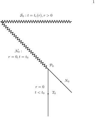
Figure 1: Local causal structure of the singularity in spherical dust collapse. We identify three different portions of the singularity; ${\cal P}_{0}$, the end-point of the time-like geodesic $T_{0}$ ($r=0,t<t_{0}$); ${\cal N}_{0}$ ($t=t_{0},r=0$), the visible portion of the singularity and ${\cal S}_{0}$ ($t=t_{c}(r),r>0$), the censored portion of the singularity. $N_{0}$ is the unique ingoing radial null geodesic terminating at ${\cal P}_{0}$.

V Structure of the singularity II: Some useful limits.

In this section, we consider the limits of various quantities along different causal geodesics terminating at and emanating from the singularity.

V.1 Causal geodesics running into the singularity

We consider first the congruence of future-pointing time-like geodesics $r=r_{0}\geq 0$ with tangent ${\vec{u}}=\frac{\partial}{\partial t}$. This is the congruence formed by the world-lines of the dust particles and $t$ is proper time along each member of the congruence. We study the approach to the singularity from the point of view of the behaviour of the characteristic lengths $l_{\alpha}$, $\alpha=1,2,3$ along the eigen-directions of the expansion tensor $\theta_{ab}=\nabla_{a}u_{b}$, defined by

$$\frac{\dot{l}_{\alpha}}{l_{\alpha}}=\theta_{\alpha},$$

where $\theta_{\alpha}$ is the eigenvalue associated with the direction $\alpha$. The geodesics in question have eigenvalues

$$\theta_{1}=\frac{R_{,rt}}{R_{,r}}=\frac{1}{3}(t_{c}-t)^{-1}-(t_{sc}-t)^{-1}$$

and

$$\theta_{2}=\theta_{3}=\frac{R_{,t}}{R}=-\frac{2}{3}(t_{c}-t)^{-1}.$$

Then the characteristic lengths $l_{\alpha}$ along $r=0$ satisfy (by virtue of $t_{c}(0)=t_{sc}(0)=t_{0}$)

$$l_{1}=l_{2}=l_{3}=(t_{0}-t)^{2/3}.$$

Thus this singularity is a ‘point’ in the Thorne classification (see e.g. chapter one of dsincosmo (5)). On the other hand, the characteristic lengths along $r=r_{0}>0$ satisfy

$$l_{1} = (t_{sc}(r_{0})-t)(t_{c}(r_{0})-t)^{-1/3}$$

$$\sim (t_{sc}(r_{0})-t_{c}(r_{0}))(t_{c}(r_{0})-t)^{-1/3},$$

$$l_{2} = l_{3}=(t_{c}(r_{0})-t)^{2/3},$$

so these singularities (i.e. the different endpoints of these geodesics) are ‘cigars’ in this classification. Apart from the issue of visibility, this is the first indication of a significant distinction between the singularities ${\cal P}_{0}$ and ${\cal S}_{0}$.

The shear and expansion scalars of this congruence are given by

$$\sigma^{2} = \frac{1}{3}((t_{sc}-t)^{-1}-(t_{c}-t)^{-1})^{2},$$

$$\theta = ((t_{sc}-t)^{-1}+(t_{c}-t)^{-1}),$$

while the density and Weyl invariant are

$$\rho = \frac{4}{3}(t_{c}-t)^{-1}(t_{sc}-t)^{-1},$$

$$\Psi_{2} = \frac{2}{9}(t_{c}-t)^{-2}(t_{sc}-t)^{-1}(t_{c}-t_{sc}).$$

The limiting behaviour of ratios of these terms have significance in the study of singularities, in particular in the context of the Weyl curvature hypothesis and the study of isotropic singularities which has grown up around this. See gw (9) for the ideas which motivate this study, and se (18) for a more recent review of the topic. The hypothesized scenario which these studies seek to corroborate or deny is that the initial cosmological singularity has low ‘gravitational entropy’ penrose (8) and consequently sub-dominant Weyl curvature, while singularities arising from the end-state of collapse are highly entropic and so are accompanied by dominant Weyl curvature.

We recall that isotropic singularities have been put forward as a model of the initial cosmological singularity, and the sub-dominance of the Weyl curvature is manifest in these models in that

$$W^{2}:=\frac{C_{abcd}C^{abcd}}{R_{ef}R^{ef}}\to 0$$ (18)

in the limit as the singularity is approached gw (9). Other limits may also be derived for the case of isotropic singularities gw (9), for example

$$\lim\{\frac{A}{\theta^{2}},\frac{\sigma^{2}}{\theta^{2}},\theta\}=\{\frac{1}{3},0,+\infty\},$$

where $A=G_{ab}u^{a}u^{b}$ and $u^{a}$ is tangent to a time-like congruence. The limit is taken along this congruence, which is assumed to have a certain degree of regularity.

Now, in the present case, along the central world-line $T_{0}$, we find the following limits:

$$\lim_{t\to t_{0}}\{W^{2},\frac{A}{\theta^{2}},\frac{\sigma^{2}}{\theta^{2}},\theta\}=\{0,\frac{1}{3},0,-\infty\},$$

which reveals an interesting comparison with isotropic behaviour summarised above. In fact, the equality holds identically for the first three limits. The sign difference in the last term arises from the fact that we are studying collapse.

Along the world-lines $r=r_{0}>0$, the corresponding limits are

$$\lim_{t\to t_{c}(r_{0})}\{W^{2},\frac{A}{\theta^{2}},\frac{\sigma^{2}}{\theta^{2}},\theta\}=\{+\infty,0,\frac{1}{3},-\infty\}.$$

Note that the shear is divergent in the approach to the singularity and that the first of these limits indicates the dominance of the Weyl curvature at ${\cal S}_{0}$. The latter actually holds for any causal curve running into ${\cal S}_{0}$. To see this we can write

$$W=\frac{1}{6}\frac{t_{sc}-t_{c}}{t_{c}-t}.$$

Since $t_{sc}(r_{0})>t_{c}(r_{0})$ for $r_{0}>0$, this quantity diverges to $+\infty$ in the approach to the singularity $t=t_{c}(r),r>0$ regardless of the direction of approach.

Again, we conclude that there is a significant difference between the behaviour at ${\cal P}_{0}$ and at ${\cal S}_{0}$.

As far as ingoing radial null geodesics are concerned it was already demonstrated in section IV that there is a unique ingoing radial null geodesic which terminates at ${\cal P}_{0}$. Repeating the arguments of the next section (from (19) onwards), we can shown that the Weyl-to-Ricci ratio $W$ is finite in the limit as the singularity is approached along this geodesic. This ratio diverges in the approach to ${\cal S}_{0}$ along ingoing radial null geodesics.

V.2 Causal curves emerging from the singularity

As we have shown above, the singularity is naked if and only if there are time-like geodesics emerging the singularity. These results only show existence of such geodesics and give very little information about them, certainly not enough to carry out the analysis done in the previous section. However, there is one situation in which this analysis is possible, namely self-similar collapse. This requires the use of a slightly different gauge from the one used above. The line-element is given by (1), but the solution for $R$ is now dj92 (19)

$$R=r(1-\lambda x)^{2/3},$$

where $x=t/r$ and $\lambda$ is a constant parameter. Note that $t=0$ is no longer a regular initial data surface, but any $t=t_{i}<0$ is such. The shell-focussing singularity occurs at $x=\lambda^{-1}$. The singularity $(r,t)=(0,0)$ is naked if and only if $0<\lambda<\lambda_{c}\simeq 0.64$ dj92 (19). In the case where the singularity is naked, the surfaces $x=$constant are space-like for $x<x_{0}$ and for $x>x_{1}$, and time-like for $x_{0}<x<x_{1}$, where $x_{0},x_{1}$ are respectively the smallest and largest positive roots of $x-R_{,r}(x)=0$. $x=x_{0}$ is the Cauchy horizon, i.e. is the first outgoing radial null geodesic emerging from the singularity. All outgoing radial null geodesics in the region $x_{0}\leq x\leq x_{1},r>0$ originate at the singularity $(0,0)$. Thus for $x_{c}\in(x_{0},x_{1})$, the curves $t=x_{c}r$,$(\theta,\phi)=$constant are time-like curves originating at the singularity. We analyse this congruence under the same headings as the previous section.

Writing $R_{,r}=(1-\lambda x)^{-1/3}(1-\lambda x)=F(x)$, this congruence has unit tangent vector field

$${\vec{u}}=\alpha(x)(x\frac{\partial}{\partial t}+\frac{\partial}{\partial r}),$$

where $\alpha(x)=(x^{2}-F^{2})^{-1/2}$. The acceleration vector field is

$${\vec{a}}=\frac{a(x)}{r}(-\frac{\partial}{\partial t}+x\frac{\partial}{\partial r}),$$

where

$$a(x)=-\frac{2}{9}\lambda^{2}\alpha^{2}F(1-\lambda x)^{-4/3}.$$

The eigenvalues of the expansion tensor are found to be all equal and are given by

$$\theta_{1}=\frac{\alpha(x)}{r}.$$

Any given member of this congruence has, from the form of ${\vec{u}}$ above,

$$\frac{dr}{d\tau}=\alpha(x_{c}),$$

and so the proper time $\tau$ satisfies $\tau=r/\alpha(x_{c})$. Thus the characteristic lengths all satisfy

$$\frac{{\dot{l}_{\alpha}}}{l_{\alpha}}=\frac{1}{\tau},$$

giving $l_{\alpha}=\tau$ for $\alpha=1,2,3$. Again we see that a visible portion of the singularity consists of a singular region which are ‘points’ in Thorne’s classification.

As the expansion tensor has three equal eigenvectors, the shear of this congruence vanishes identically. The Weyl-to-Ricci ratio is

$$|\frac{\Psi_{2}}{\rho}|=\frac{1}{3}(1-\lambda x)^{-1},$$

which is non-zero and finite in the limit as the singularity is approached along $x=x_{c}$. $\Psi_{2}$ and $\rho$ both individually diverge at the singularity. The expansion $\theta=3\alpha(x)/r$ diverges.

In the general (i.e. non-self similar case), we can analyze this last limit for the time-like geodesics emerging from the singularity whose existence has been proven in Proposition 3 above. The limit we wish to determine is

$$W_{0} = \lim_{r\to 0}|\frac{\Psi_{2}}{\rho}|$$

$$= \lim_{r\to 0}\frac{1}{6}\frac{t_{sc}-t_{c}}{t_{c}-t},$$

where the limit is taken along the geodesic emerging from the singularity. The value of this limit may be obtained using l’Hopital’s rule:

$$W_{0}=\lim_{r\to 0}\frac{1}{6}\frac{t^{\prime}_{sc}-t^{\prime}_{c}}{t^{\prime}_{c}-t^{\prime}},$$ (19)

where $t^{\prime}$ is the slope of the geodesic in the $r-t$ plane. Referring to the proof of Proposition 9 in mn1 (2), we recall that along such geodesics, the slope $t^{\prime}(r)$ of these curves in the $r-t$ plane satisfies

$$R_{,r}\leq t^{\prime}\leq(1+\delta)R_{,r},$$

for some $\delta>0$ and sufficiently small. The significance of $R_{,r}$ is that it gives the slope of the outgoing radial null geodesics and therefore the bounds above allow us to focus on the radial null geodesics. We know that such geodesics emerge into the region $t_{0}<t<t_{H}(r)$, where $t=t_{H}(r)=t_{c}-\frac{2}{3}m$ is the apparent horizon. Using the latter bounds on $t$, we can obtain bounds on $R_{,r}$ (see equation (17)), i.e. on $t^{\prime}$. These in turn may be integrated to improve the original bounds on $t$. Focussing on the case where $m^{\prime}_{1}(0)\neq 0$ and carrying out this process twice yields bounds of the form

$$c_{1}r^{2/3}+u_{1}(r)\leq t^{\prime}\leq c_{2}r^{2/3}+u_{2}(r),$$

where $0<c_{1}<c_{2}$ and $u_{i}=o(r^{2/3})$ for $i=1,2$. We can then take the limit in (19) and find that

$$W_{0}=\lim_{r\to 0}\frac{1}{6}\frac{t^{\prime}_{sc}-t^{\prime}_{c}}{t_{c}^{\prime}-t^{\prime}}=\frac{1}{9}.$$

In the case $m^{\prime}_{1}(0)=0,m^{\prime\prime}_{1}(0)\neq 0$, the limit gives $W_{0}=2/9$. These limits are the same for every causal geodesic emerging from the singularity. Finally, for the case $m^{\prime}_{1}(0)=m^{\prime\prime}_{1}(0)=0$, $m^{\prime\prime\prime}_{1}(0)\neq 0$, the existence of the limit is proved in the same way as above. In this case, the result depends on the value of the third derivative and on the geodesic in question.

Our principal conclusion is thus that the visible portion ${\cal N}_{0}$ of the singularity does not exhibit the Weyl-dominance which is thought to be characteristic of singularities arising in collapse. Nor does it exhibit the Weyl-sub-dominance (18) characteristic of isotropic singularities. In the case where the calculation may be carried out, the singularity is point-like.

As an aside, we remark that we can find examples where the quantity $W^{2}$ increases or decreases with time depending on the geodesics under consideration. This is potentially of interest to debates on gravitational entropy (see e.g. penrose (8), bonnor (20) and mt (21)) .

V.3 Redshift

In order to make contact with recent results given in desh (3) we study briefly the redshift along outgoing geodesics.

Consider a photon which is emitted by a source with unit time-like tangent $u^{a}_{(s)}$ and received by an observer with tangent $u^{a}_{(o)}$. Let $k^{a}$ be the tangent to the photon’s world-line. Then the redshift $z$ relative to the emission and reception events $P_{1}$ and $P_{2}$ is given by

$$1+z=\frac{[k_{a}u^{a}_{(s)}]_{P_{1}}}{[k_{a}u^{a}_{(o)}]_{P_{2}}}.$$

The redshift of photons emerging from a naked singularity has been calculated in dwivedi98 (22) and desh (3) for various trajectories. The source and receiver are taken to be co-moving with the fluid: take the source to be $r=r_{0}<<1$ and the receiver to be $r=r_{1}>r_{0}$. Thus the source hugs the central world-line $T_{0}$ and the null singularity ${\cal{N}}_{0}$ and terminates at ${\cal{S}}_{0}$ near to the junction of ${\cal{N}}_{0}$ and ${\cal{S}}_{0}$. Then $u^{a}_{(s)}=u^{a}_{(o)}=\delta^{a}_{0}$, and $1+z={\dot{t}}_{P_{1}}/{\dot{t}}_{P_{2}}$. Taking $P_{1}$ to be the past endpoint of a geodesic emerging into the future from the singularity places the photon source on the singularity and can be thought of as allowing $r_{0}\downarrow 0$. In dwivedi98 (22), it was shown that the redshift thus measured is finite for singularities of classes (i) and (ii) of section II, but infinite for singularities of class (iii). In desh (3), the redshift is shown to be infinite for photons propagating along non-radial geodesics emerging from the singularity. This latter result is immediate as we see from (15): ${\dot{t}}$ diverges at the singularity $R=0$ for any non-radial causal geodesic which is not a radial null geodesic. This shows that the result - infinite redshift -also applies to particle de Broglie wavelengths ($k^{a}$ time-like). This is a possible (classical) indication that particles emerging from a naked singularity may not be associated with the transfer of infinite amounts of energy. Furthermore, if physical particles escaping from the singularity always travel along geodesics with some angular momentum, then they will always be infinitely redshifted to an outside observer. We emphasize that these results are purely classical and it would be interesting to study them using e.g. a semi-classical approximation.

VI Structure of the singularity III: Topology

In the previous section, we classified the different portions of the singularity using Thorne’s point-cigar-barrel-pancake classification. This describes the behaviour of a co-moving fluid element carried by a time-like congruence meeting the singularity. However, this does not address another question which relates to the topology of the singularity and which we shall now describe. In the conformal diagram of Figure 1, each point in the two-dimensional representation of the non-singular part of the space-time manifold represents a 2-sphere: the point $(r,t)$ of this diagram represents the 2-sphere with radius $R=R(r,t)$ at time $t$. The question we address here is the following: does each point on the singular boundary ${\cal P}_{0}\cup{\cal N}_{0}\cup{\cal S}_{0}$ represent topologically a 2-sphere or a point? Christodoulou has shown that the future outgoing null (and hence censored) singular boundary which can arise in the collapse of a self-similar scalar field is foliated by points, while the space-like singular boundary that arises in another sector of the space of solutions is foliated by 2-spheres christo-scalar (6).

Christodoulou’s argument runs as follows. Any radial null geodesic of the space-time actually represents a 2-sphere’s worth of null geodesics. Consider a radial null geodesic $\gamma$ running into a future outgoing null singular boundary ${\cal N}_{1}$. This actually represents a family $\gamma^{\xi},\xi\in\bf{S}^{2}$ of radial null geodesics running into the singularity. From this family, choose a fixed member $\gamma^{N}$ and the antipodal member $\gamma^{S}$ ($N,S$ for north, south). Now let $\{p^{N,S}_{n}\}$ be causally increasing sequences of points along $\gamma^{N,S}$ respectively, chosen so that the singularity is reached in the limit $n\to\infty$ and for each $n$, the points $p^{N,S}_{n}$ are antipodal on the same 2-sphere $\bf{S}^{2}_{n}$ . Christodoulou shows that the causal pasts $J^{-}(p^{N,S}_{n})$ of $p^{N,S}_{n}$ satisfy

$$\lim_{n\to\infty}J^{-}(p^{N}_{n})=\lim_{n\to\infty}J^{-}(p^{S}_{n}),$$

and so the ideal boundary points $\lim_{n\to\infty}p^{N,S}_{n}$, having the same causal past, are, by definition, identical. See Figure 2.

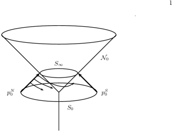
Figure 2: Behaviour of non-radial geodesics near the singularity. For convenience, we consider a future outgoing null singular boundary ${\cal N}_{0}$. $R=0$ along ${\cal N}_{0}$. The straight arrows represent ingoing radial null geodesics $\gamma^{N,S}$ with initial points $p^{N,S}_{0}$ which are antipodal points on an initial 2-sphere $S_{0}$. These geodesics project to the same radial null geodesic in the Lorentzian 2-space $d\Omega=0$. The curved arrows are past-directed non-radial null geodesics emerging from different points $p^{N}_{n}\in\gamma^{N}$, the different lengths of these curves representing the fact that angular velocity ${\dot{\phi}}$ of these geodesics increases as their initial point $p^{N}_{n}$ approaches the singularity $R=0$. In the case where $\phi\to-\infty$ as the singularity is approached, the geodesics reach all the way around the regular center $R=0$ to the opposite side, and in the limit, we may consider that the non-radial geodesic emitted from $p^{N}_{\infty}$ reaches $p^{S}_{\infty}$. Hence as points of the causal boundary, $p^{N}_{\infty}$ and $p^{S}_{\infty}$ are identified and $S_{\infty}$ is a single point. In the case where $\phi$ has a finite limit as the singularity is approached, $S_{\infty}$ is a 2-sphere.

The key ingredient required for this argument is to show that past-directed non-radial null geodesics through $p^{N}_{n}$ orbit the axis $R=0$ sufficiently quickly (in the limit as $n\to\infty$) so that the causal past of $p^{S}_{n}$ is contained in the causal past of $p^{N}_{n}$. That is, the rapidly orbiting non-radial null geodesics have enough ‘time’ to get around from the north to the south pole of $\bf{S}^{2}_{n}$ and so have a look at what is to be seen from there. See Figure 2.

We argue here that, at least in the self-similar case, the topology of the naked portion of the singularity is not uniform, being point-like on one region and spherical on another. This requires a fairly thorough analysis of the behaviour of null geodesics emerging from the singularity.

In the self-similar case, the line element may be written (see e.g. dj92 (19))

$$ds^{2}=-dt^{2}+F^{2}(x)dr^{2}+r^{2}U^{2}(x)d\Omega^{2},$$ (20)

where $x=t/r$ and

$$U(x)=(1-\lambda x)^{2/3},\qquad F(x)=(1-\lambda x)^{-1/3}(1-\frac{\lambda}{3}x).$$

The shell-focussing singularity occurs at $x=\lambda^{-1}$. The equations governing outgoing radial null geodesics (ORNG’s) may be written as

$$\frac{dx}{dr}=\frac{F-x}{r}.$$

Then it can be shown that the singularity is naked for $\lambda$ in the range $(0,\lambda_{c})$, in which case $F-x$ has two positive roots $x_{0}<x_{1}<\lambda^{-1}$. The curves $x=x_{0}$ and $x=x_{1}$ are outgoing radial null geodesics emerging from the singularity $(t,r)=(0,0)$. We recall that $x_{0}$ corresponds to the Cauchy horizon, i.e. the boundary of the future of a regular initial data surface $t=t_{i}<0$.

ORNG’s initially in the region $x\in(x_{0},x_{1})$ remain in this region and satisfy $x^{\prime}(r)=(F-x)/r<0$. Thus along such a geodesic, $x$ increases as $r\downarrow 0$. But $x$ is bounded above by $x_{1}$, and so must have a finite limit as $r\downarrow 0$. This limit $(\lim\frac{t}{r}=\lim\frac{dt}{dr})$ must solve $x=F$ and so must equal $x_{1}$. A similar argument applies for ORNG’s in $x\in(x_{1},\lambda^{-1})$. Hence all ORNG’s emerging from the singularity, except for the single ORNG $x\equiv x_{0}$, originate at $(0,0)$ with $x=x_{1}$. However as we will see, non-radial null geodesics may emerge with different values of $x$ in this limit. We note that this indicates that considering only radial null geodesics does not give a complete picture of the singular boundary.

We now consider the question raised above. Each of the radial null geodesics emerging from $(0,0)$ represents a 2-sphere’s worth of ORNG’s emerging from the singularity. To address the issue of the topology of the singularity, we consider non-radial null geodesics (NRNG’s) emerging from the singularity.

The homothetic Killing vector field which generates the self-similarity of (20) is

$$\vec{\xi}=t\frac{\partial}{\partial t}+r\frac{\partial}{\partial r}.$$

If $k^{a}$ is tangent to a null geodesic, then $g_{ab}\xi^{a}k^{b}$ is constant along the geodesic. This is a first integral of the null geodesic equations, which we may therefore write as

$$-{\dot{t}}^{2}+F^{2}{\dot{r}}^{2}+\frac{L^{2}}{r^{2}U^{2}} = 0,$$ (21)

$$-{\dot{t}}+\frac{F^{2}}{x}{\dot{r}}+\frac{k}{rx} = 0,$$ (22)

where $L$ is the conserved angular momentum and $k$ is the constant generated by $\vec{\xi}$. We can assume that $k\geq 0$, as a change of sign in $k$ corresponds to a change in sign of the affine parameter. Our principal result which is of significance for the topology of the singularity is the following:

Proposition 5

(i) Through every point of $\{(t,r):x_{0}<x<x_{1}\}$, there exists a non-radial null geodesic which emerges from the singularity $(0,0)$. Along this geodesic, ${\dot{\phi}}$ is a non-integrable function of the affine parameter $\tau$, and $\phi$ diverges to $-\infty$ in the limit as the singularity is approached.
(ii) Through every point of $\{(t,r):x_{1}<x<\lambda^{-1}\}$, there exist non-radial null geodesics which emerge from the singularity $(0,0)$. Along every such geodesic, $\phi$ has a finite limit as the singularity is approached.

The proof is given in the appendix. Proposition 5 allows us to deduce the following results regarding the topological nature of the singularity ${\cal{N}}_{0}$, from the causal boundary perspective.

We start by recalling that radial null geodesics emerge into the region $x_{0}<x<x_{1}$. Now, on any such geodesics, we may choose a point $p^{N}$ sufficiently close to the singularity such that there exists a non-radial null geodesic through $p^{N}$ with the property than this NRNG reaches the antipodal point of the 2-sphere (on which $p^{N}$ lies) before the radial geodesic reaches the singularity. The significance of this is that in the limit as the point $p^{N}$ approaches the singularity, this point and its antipodal partner $p^{S}$ must be considered to have the same causal future, and so are identified as points of the causal boundary. Therefore, the corresponding section of ${\cal{N}}_{0}$ is foliated by points.

On the other hand, the results obtained for NRNG’s in the region $x_{1}<x<\lambda^{-1}$ indicate that the NRNG’s through a point $p^{N}$ do not have enough time to reach the antipodal point $p^{S}$ before the singularity is reached. Hence in the limit as the singularity is approached, the causal futures of $p^{N}$ and $p^{S}$ will not match up with one another, and hence these points cannot be identified as points of the causal boundary. In fact $p^{N}$ will not have the same limiting causal future as any other point on the same 2-sphere, and so the corresponding portion of ${\cal N}_{0}$ is foliated by 2-spheres.

Finally, one further point of relevance may be deduced from the proof of Proposition 5: In every case considered, the future evolution of the NRNG’s terminates at $x=\lambda^{-1}$ at some $r>0$. The limiting behaviour of ${\dot{r}}$ and ${\dot{x}}$ in terms of $x$ can be read off from the governing equations, and can be used to obtain the limiting behaviour of ${\dot{R}}={\dot{r}}U+rU^{\prime}{\dot{x}}$. This can be integrated, and generically yields a result indicating integrability of $1/R^{2}$. Hence $\phi$ has a finite limit along any NRNG approaching the singularity $x=\lambda^{-1}$ at some $r>0$. Thus the singularity ${\cal S}_{0}$ is foliated by 2-spheres.

VII Conclusions and comments

We have extended the result of mn1 (2) to all f.p. causal geodesics by proving that for the marginally bound spherical dust collapse there are radial and non-radial timelike geodesics which emanate from the ensuing singularity if and only if there are radial null geodesics which emanate from the singularity. It remains to be seen whether this result is true in general in spherical symmetry, at least for singularities at zero radius. The fact that the naked singularity always has time-like geodesics emerging therefrom leads to interesting possibilities in terms of the spectrum of particles that may be created by such a singularity: such particles may be massive as well as massless. This would seem to be vital if the information lost in the process of collapse is to re-emerge at a later stage in the form of a black hole or naked singularity explosion Harada-etal00 (23).

We have studied the structure of the singularity from several points of view. We started by studying the behaviour of limits of various quantities along causal geodesics terminating at the singularity and emanating from the singularity. In this way we have classified different sectors of the singularity as points and cigars. We have then considered the topological properties of the singularity. These studies were motivated by the fact that the existence of non-radial null geodesics emerging from the singularity suggests that it must have some non-pointlike structure. Naively, one might expect that the singularity ${\cal N}_{0}$ of Figure 1 must by cylindrical, i.e. foliated by 2-spheres, since points thereon emit a full 2-spheres worth of non-radial null geodesics. This is in contrast to a regular center of a spherically symmetric space-time, through which non-radial null geodesics cannot pass. However detailed calculations indicate that while the topology of ${\cal S}_{0}$ is that of a 2-sphere, the topology of ${\cal N}_{0}$ (in the sense of ideal boundary points) may be either that of a 2-sphere or of a point.

The calculations in section V of various limits at the singularity seem to us to be of interest beyond merely classifying the different portions of the singularity. The question of what constitutes a genuine space-time singularity is not yet settled. This is of particular relevance for cosmic censorship hypothesis: a visible singularity which is mild in some suitably (and rigorously) defined way should not be considered a counter-example to the hypothesis. The following two definitions have proved to be useful. Both involve the question of predictability to the future of a singularity.

We mention first that of Clarke clarke (24). Put simply, a singularity is considered inessential if it does not present any obstruction to the evolution of test fields in space-time. The question of global hyperbolicity of the space-time (cosmic censorship) is redirected to the question of generalized hyperbolicity of fields on the space-time. Examples of space-times admitting singularities in the classical sense of $C^{2-}$ geodesic incompleteness but satisfying a generalized hyperbolicity condition have been given in clarke (24), vic-wil1 (25) and vic-wil2 (26).

The second definition is that of an isotropic singularity gw (9). As mentioned above, this was introduced in the study of the initial cosmological singularity and hypotheses related to this penrose (8). The connection with cosmic censorship is perhaps not immediately obvious, but becomes so when one acknowledges that the initial cosmological singularity is naked: every past-directed causal geodesic meets the singularity. The isotropic singularity program has produced the following profound result: the big bang can be considered a regular initial data surface for the Einstein field equations. (Different matter models have been studied; polytropic perfect fluids in ang-tod1 (27), the Einstein-Vlasov model in ang-tod2 (28). These rely on results for singular differential operators due to Newman-Claudel new-claud (29).) Thus with isotropic singularities, we see that it is possible to have global hyperbolicity of the space-time to the future of a singularity.

So with a view to addressing the question of whether or not the naked singularities studied here should be considered genuine counter-examples to cosmic censorship we could ask: do we have any evidence that the singularity is either (i) inessential in Clarke’s sense or (ii) isotropic? We will not address the first of these here. Regarding the second, we contend that there is some evidence that, at least in the self-similar case, the singularity ${\cal{N}}_{0}\cup{\cal{P}}_{0}$ has characteristics in common with isotropic singularities.

As we have seen, the Weyl-sub-dominance property (18) - a characteristic of isotropic singularities - is not satisfied for the congruence of time-like curves emerging from the singularity which we studied in Section 5.2. Nevertheless, we speculate that the fact that the ratio $W^{2}$ is finite (but not zero) may turn out to be an indication of good behaviour of ${\cal N}_{0}$ regarded as an initial data surface. As evidence in favour of this, consider the following details which relate again to the self-similar case. From the calculations in the appendix, we know that outgoing radial null geodesics emerging from the singularity fall into two classes. The first class contains a single member, the ORNG $x=x_{0}$, which emerges from ${\cal P}_{0}$ in Figure 1. The second class consists of all other ORNG’s emerging from the singularity: these emerge from ${\cal N}_{0}$. Along these geodesics, the limit $x\to x_{1}$ is satisfied as the singularity is approached. Hence the congruence of time-like curves $x=x_{c}\in(x_{0},x_{1})$ - call it the similarity congruence - considered in §V.B must be considered to emerge from ${\cal P}_{0}$. This resembles the behaviour of the initial singularity in certain FLRW universes, namely those filled with a perfect fluid satisfying a equation of state $p=\alpha\rho$, with $\alpha\in(-1,-1/3]$. In these space-times, the entire fluid congruence emerges from a single point of the singularity and a null portion of the singularity forms a portion of the causal future of this point. See seno (4) for details. This resemblance is borne out by writing the line-element in coordinates adapted to the similarity congruence. Introduce a time function $T=rH(x)$ chosen so that the similarity congruence is orthogonal to $T=$constant. Then the line-element becomes

$$ds^{2}=\frac{r^{2}}{(x^{2}-F^{2})}\left\{-(x^{2}-F^{2})^{2}\frac{dT^{2}}{T^{2}}+F^{2}dx^{2}+U^{2}d\Omega^{2}\right\}.$$

This applies for $r>0$ and $x\in(x_{0},x_{1})$, wherein $x^{2}-F^{2}>0$. The function $H$ satisfies

$$\frac{H^{\prime}}{H}=\frac{x}{x^{2}-F^{2}},$$

and therefore is finite on $(x_{0},x_{1})$. The line-element may be written as $ds^{2}=T^{2}d\bar{s}^{2}$, where

$$d\bar{s}^{2}=-a^{2}(x)\frac{dT^{2}}{T^{2}}+b^{2}(x)dx^{2}+c^{2}(x)d\Omega^{2},$$

with $a,b,c$ finite and non-zero on $(x_{0},x_{1})$. $T$ is the exponential of proper time along the similarity congruence. This decomposition of the metric into an overall scaling factor (which vanishes at the singularity) times a non-singular metric (when written in terms of $\tau=\ln T$) is exactly the same decomposition which exists for the FLRW metrics mentioned above, and is similar to the decomposition whose existence defines isotropic singularities (the difference is that $\tau\to-\infty$ at the singularity currently under discussion).

So while there is still no direct evidence that this naked singularity does not break the future predictability of the space-time, the question appears to be worthy of future investigation.

Appendix A Proof of proposition 5

(i) Given $x_{c}\in(x_{0},x_{1})$, it is straightforward to show that there are NRNG’s confined to this time-like hypersurface which have the desired properties. Substituting $x=$constant into (21) and (22) yields

$$r{\dot{r}}=\pm\frac{L}{U}(x^{2}-F^{2})^{-1/2}=k(x^{2}-F^{2})^{-1},$$

which is valid since $x^{2}>F^{2}$ in $(x_{0},x_{1})$. Choosing $k,L$ so that these two match, which gives a 1-parameter solution, gives the geodesic in question. A sign choice is required in order that the geodesic is future pointing ${\dot{t}}>0$. Note that $r{\dot{r}}=c$, which is positive for the future-pointing choice and so $r^{2}\sim 2c\tau$ as $\tau\downarrow 0$, choosing the origin of the affine parameter $\tau$ to coincide with the singularity. Then

$${\dot{\phi}}\sim\frac{L}{2c}\tau^{-1},$$

and so $\phi$ diverges to $-\infty$ as the singularity is approached.

(ii) To prove this part of the proposition requires the study of all non-radial null geodesics in the region $(x_{1},\lambda^{-1})$. The equations (21) and (22) yield a quadratic equation for ${\dot{r}}$, which has solutions given by

$$r{\dot{r}}=\frac{1}{F^{2}-x^{2}}[-k\pm\frac{x}{F}(k^{2}+\frac{L^{2}}{U^{2}}(F^{2}-x^{2}))^{1/2}].$$ (23)

These give

$${\dot{x}}=\pm\frac{1}{r^{2}F}(k^{2}+\frac{L^{2}}{U^{2}}(F^{2}-x^{2}))^{1/2}.$$ (24)

The solutions with the lower sign require the change $\tau\to-\tau$ in order to be explicitly future-pointing. Implementing this, the equations are (any two of)

$$r{\dot{r}} = \frac{1}{F^{2}-x^{2}}[k+\frac{x}{F}(k^{2}+\frac{L^{2}}{U^{2}}(F^{2}-x^{2}))^{\frac{1}{2}}]>0,$$ (25)

$${\dot{x}} = \frac{1}{r^{2}F}(k^{2}+\frac{L^{2}}{U^{2}}(F^{2}-x^{2}))^{1/2}>0,$$ (26)

$${\dot{t}} = \frac{F^{2}}{x}{\dot{r}}-\frac{k}{rx}>0.$$ (27)

Recall that $k\geq 0$. Positivity of ${\dot{x}}$ immediately gives

$$t<x_{i}r$$ (28)

for any point $(t,r)$ preceding a chosen initial point $(t_{i},r_{i})$. Positivity of ${\dot{r}}$ and $k$ yields

$$r\frac{dx}{dr} < \frac{F^{2}-x^{2}}{x}$$

$$< 2(F^{\prime}_{1}-1)(x-x_{1})+M(x-x_{1})^{2}.$$

There latter inequality arises from using Taylor’s theorem on $F$, which is analytic at $x_{1}$. $2M>0$ is a bound on the closed interval $[x_{1},x_{i}]$ of the (continuous) second derivative of $(F^{2}-x^{2})/x$. $F^{\prime}_{1}=F^{\prime}(x_{1})$, and this number is always bigger than 1. Integrating over $[r,r_{i}]$, where $0<r<r_{i}$ yields

$$t>x_{1}r+(\frac{c_{1}}{1-c_{2}r^{A}})r^{A+1},$$ (29)

where $c_{1,2}$ are positive constants and $A=2(F^{\prime}_{1}-1)>0$. Combining (28) and (29), we see that these geodesics all originate at $(t=0,r=0)$.

The rate at which $r$ shrinks to zero can be obtained as follows. We have

$$r{\dot{r}}\sim\frac{2k}{F^{2}-x^{2}}\sim\frac{k}{x_{1}(F^{\prime}_{1}-1)}(x-x_{1})^{-1},$$

while

$${\dot{x}}\sim\frac{k}{x_{1}}r^{-2}.$$

These may be integrated to give

$$r\sim k\tau^{1/(F^{\prime}_{1}+1)}=k\tau^{\alpha}$$

where $\alpha<1/2$ and so

$$\phi(\tau)=\int_{0}^{\tau}\frac{L}{R^{2}(\nu)}\,d\nu$$

converges to a finite value in the limit as $\tau\downarrow 0$.

Next we consider the solutions corresponding to the choice of upper sign in (23) and (24). We note that ${\dot{t}}>0$ and ${\dot{x}}>0$ are automatic consequences of this choice. On the other hand, ${\dot{r}}>0$ if and only if $H(x)>0$, where

$$H=\frac{L^{2}}{U^{2}}-\frac{k^{2}}{x^{2}}.$$

We note that $H^{\prime}(x)>0$. Then for any initial value $H(\tau_{0})$ of $H$, the increase of $x$ brings about the increase of $H$ to positive values. Then ${\dot{r}}$ becomes and remains positive, and so the geodesic must run into the singularity $x=\lambda^{-1}$. The past evolution requires more careful attention. We deal with the case $k>0$ first.

We have $r{\dot{r}}=r{\dot{r}}(x)$, and by using a Taylor expansion centered on $x_{1}$, we find

$$r{\dot{r}}(x)=\frac{H(x_{1})}{2k}+O(x-x_{1}).$$

If in the past evolution we reach $\tau_{1}<\tau_{0}$ whereat $H(\tau_{1})<0$ and $x(\tau_{1})>x_{1}$, then $H<0$ for all $\tau<\tau_{1}$. Hence $r$ increases into the past, and so the geodesic inevitably extends back to $x=x_{1}$ at some $r>0$, thus avoiding the singularity. This situation is obtained if and only if $H(x_{1})<0$.

So it remains to consider the cases $H(x_{1})\geq 0$. If $H(x_{1})>0$, then the argument above shows that $r{\dot{r}}>0$ for all $x>x_{1}$.

We can obtain the bound $rx^{\prime}(r)>(F^{2}-x^{2})/x$. Integrating over $[r,r_{i}]$ ($0<r<r_{i}$) yields

$$\int_{r}^{r_{i}}\frac{x}{F^{2}-x^{2}}\,dx>\ln|\frac{r_{i}}{r}|.$$

Thus if the geodesic approaches $r=0$ in the past, then the integral on the left hand side here must diverge. This can only occur if we also have $x\downarrow x_{1}$ as the singularity is approached. Let this occur at $\tau=\tau_{s}$. But then

$$x_{1} = \lim_{\tau\to\tau_{s}}\frac{t}{r}$$

$$= \lim_{r\to 0}\frac{dt}{dr}$$

$$= \lim_{x\to x_{1}}(\frac{F^{2}}{x}+\frac{k}{xr{\dot{r}}})$$

$$= x_{1}+2\frac{k^{2}}{x_{1}}(\frac{L^{2}}{U_{1}^{2}}-\frac{k^{2}}{x_{1}^{2}})^{-1},$$

which yields a contradiction. Therefore these geodesics must extend back to $x=x_{1}$ before reaching $r=0$. This argument applies when $H(x_{1})>0$ and requires only slight modification to be applied to the case $H(x_{1})=0$. Note that there is a finite (rather than infinitesmal) interval of affine parameter between an initial point on the geodesic and the point corresponding to entry into the region $x\leq x_{1}$.

Finally, we need to consider the NRNG’s with $k=0$. Note that in this case, the choice of sign in (23) and (24) is only of a time-orientation and so without loss of generality we only treat the choice of upper sign. The argument leading up to (29) may be repeated to show that in this case, there exist geodesics emerging from $(0,0)$, and that $x\to x_{1}$ along these geodesics as the singularity is approached. It remains to determine the rate at which $r$ approaches zero for these geodesics.

From the governing equations, we have ${\dot{x}}=G(x)r^{-2}$, where

$$G(x)=\frac{L}{FU}(F^{2}-x^{2})^{1/2}.$$

We can also write

$$(r^{2})^{\cdot}=2r^{2}x(F^{2}-x^{2})^{-1}{\dot{x}}.$$

These yield the second order equation

$${\ddot{x}}=J(x){\dot{x}}^{2},$$

where

$$J(x) = (\frac{G^{\prime}}{G}-\frac{2x}{F^{2}-x^{2}})$$

$$= \frac{1}{2}(\frac{F^{\prime}_{1}-3}{F^{\prime}_{1}-1})(x-x_{1})^{-1}+O(1)\quad\hbox{{\rm as}}\quad x\to x_{1}.$$

This equation may be integrated to obtain the $\tau-$dependence of $x$ as $x\downarrow x_{1}$. Then using $r^{2}=H/{\dot{x}}$, we obtain

$$r^{2}\sim c^{2}\tau^{2/(F^{\prime}_{1}+1)}\quad\hbox{{\rm as}}\quad r\to 0.$$

Recalling that $F^{\prime}_{1}>1$, we see that the power here is less than one. Hence

$${\dot{\phi}}=\frac{L}{R^{2}}\sim\frac{L}{U^{2}(x_{1})r^{2}}$$

is integrable in the limit as the singularity is approached, giving a finite limit for the value of $\phi$.

To summarise: NRNG’s in $x>x_{1}$ either exit this region at some finite radius, taking a finite amount of time to do so, or emerge from the naked singularity $(0,0)$. In the latter case, $\phi$ has a finite limit in the approach to the singularity. This concludes the proof of the proposition.

References

- (1) Singh T P & Joshi P S 1996 Class. Quantum Grav. 13 559
- (2) Mena F C & Nolan B C 2001 Class. Quantum Grav. 18 4531.
- (3) Deshingkar S S, Joshi P S & Dwivedi I W, 2001. Appearance of the central singularity in spherical collapse. To appear in Phys. Rev. D Published electronically as gr-qc/0111053.
- (4) Senovilla J M M, 1998 Gen. Rel. Grav. 30 701
- (5) Wainwright J & Ellis G F R (eds.) 1997 Dynamical Systems in Cosmology (Cambridge: Cambridge university Press)
- (6) Christodoulou D, 1994 Ann. Math. 140 607.
- (7) Scott S & Szekeres P, 1986 Gen. Rel. Grav., 18 557
- (8) Penrose R, in General Relativity: An Einstein Centenary Survey, eds. Hawking S W & Israel W, (Cambridge: Cambridge University Press, 1979)
- (9) Goode S W & Wainwright J 1985 Class. Quantum Grav., 2 99.
- (10) Lemaitre G 1933 Ann. Soc. Sci. Bruxelles, A53 51
- (11) Tolman R C 1934 Proc. Nat. Acad. Sci., 20
- (12) Bondi H 1947 Mon. Not. R. Astron. Soc., 107 410
- (13) Eardley D M & Smarr L 1979 Phys. Rev. D19 2239
- (14) Christodoulou D 1984 Commun. Math. Phys. 93 171
- (15) Newman R P A C 1986 Class. Quantum Grav. 3 527
- (16) Nolan B C 1999 Phys. Rev. D60 024014
- (17) Nolan B C, Mena F C & Gonçalves S M C V 2002 Phys. Lett. A 294, 122.
- (18) Scott S M & Ericksson G 1998 in Current Topics in Mathematical Cosmology ed. M Rainer and H-J Schmidt (Singapore: World Scientific)
- (19) Dwidevi I H & Joshi P S 1992 Commun. Math. Phys. 146 333
- (20) Bonnor W B 1985 Phys. Lett. A 112 26
- (21) Mena F C & Tavakol R 1999 Class. Quant. Grav. 16 435
- (22) Dwivedi I H 1998 Phys. Rev. D 58 064004
- (23) Harada T, Iguchi H & Nakao K, 2000 Phys.Rev. D 61 101502; ibid. 62 084037.
- (24) Clarke C J S 1998 Class. Quantum Grav. 15 975.
- (25) Vickers J A & Wilson J P 2000 Class. Quantum Grav. 17 1333.
- (26) Vickers J A & Wilson J P 2001 Generalised hyperbolicity: hypersurface singularities University of Southampton preprint. Published electronically as gr-qc/0101018.
- (27) Anguige K & Tod K P 1999 Ann Phys. (NY) 276, 257.
- (28) Anguige K & Tod K P 1999 Ann Phys. (NY) 276, 294.
- (29) Claudel C M & Newman K P 1998 Proc. Roy. Soc. Lond. 454, 1073.