Gravitational waves from inspiraling binary black holes
Abstract
Binary black holes are the most promising candidate sources for the first generation of earth-based interferometric gravitational-wave detectors. We summarize and discuss the state-of-the-art analytic techniques developed during the last years to better describe the late dynamical evolution of binary black holes of comparable masses.
Summary talk given at the Edoardo Amaldi Conference on Gravitational Waves, Perth, Australia, 8-13 July 2001, to appear in Special Issue Article of Classical and Quantum Gravity
1 Introduction
Binary systems made of compact objects (neutron stars or black holes) that spiral in toward coalescence because of gravitational-radiation damping are among the most promising candidate sources for interferometric gravitational-wave (GW) detectors, such as the Laser Inteferometric Gravitational Wave Observatory (LIGO), VIRGO, GEO and TAMA [1]. The inspiral waveform will enter the detector frequency band during the last few minutes or seconds of evolution of the binary and the GW community plans to track the signal phase and build up the signal-to-noise ratio by integrating the signal for the time during which it stays in the detector bandwidth. This is achieved by filtering the detector output with a template which is an (approximate) theoretical copy of the observed signal.
Einstein theory predicts that the radiative transverse traceless (TT) gravitational field , far away from the source, is related to the motion and the structure of the source, at lowest order in the post-Newtonian (PN) expansion, by the quadrupole formula
| (1) |
where () is the tracefree quadrupole moment of the source; is the distance from the source; is the unit vector from the source to the observer; is the TT projection operator onto the plane orthogonal to ; is the Newton constant; and is the speed of light. From Eq. (1) (and its extensions at higher PN orders) we see that the more precisely we know the two-body motion, the more accurately the PN template will describe the “real” gravitational waveform.
In Fig. 1 we show a typical gravitational waveform. The part of the waveform drawn with a continuous line is emitted during the inspiral phase when the two black holes are largely separated, e.g., where we denoted by the radial separation and by the total mass of the binary system. During the inspiral, the two black holes follow an adiabatic sequence of quasi-circular orbits. The equation of motion in the center-of-mass frame can be written schematically as
| (2) |
where denotes the separation vector between the two bodies and . Equation (2) is characterized by a double expansion: in the PN parameter , and in the parameter , where and are the masses of the two black holes. The parameter ranges between (test-mass limit) and (equal-mass case).
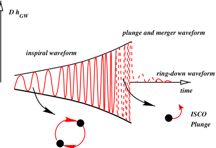
It is well known that the PN expansion converges badly: as the two bodies draw closer, and enter the nonlinear, strong curvature phase, the motion becomes relativistic, e.g., , and it is more and more difficult to extract reliable information from the PN series. More specifically, when the distance between the inspiraling black holes shrinks to , the PN expansion can no longer be trusted [2]. The dashed line in Fig. 1 depicts the (less known) part of the waveform emitted during the final phase of evolution, when nonlinearities and strong curvature effects become important and nonperturbative analytical and/or numerical techniques should be used to describe it. This final phase includes the transition from adiabatic inspiral to plunge, beyond which the two-body motion is driven (almost) only by the conservative part of the dynamics. For nonspinning binary black holes, the plunge starts at the innermost stable circular orbit (ISCO) of the binary black holes. Beyond the plunge the two black holes merge, forming a Kerr black hole. As the system reaches the stationary Kerr state, the nonlinear dynamics of the merger resemble more and more the oscillations of the black-hole quasi-normal modes [3] and the gravitational signal will be a superposition of exponentially damped sinusoids (ring-down waveform). However, if the black holes carry a big spin, it is likely that the plunge stage will never be reached and the late dynamical phase will be much more complicated in this case.
Likely, the first detection of gravitational waves with LIGO/VIRGO interferometers will come from binary systems made of black holes of comparable masses, say with a total mass . In fact, if we assume binary black holes are originated by “population synthesis” [4], the estimated detection rate per year is at [5], while if globular clusters are considered as “machines” for making binary black holes [6] the detection rate per year is at [5]. These numbers, especially the latter, are more optimistic than the estimated detection rate per year for neutron star binaries, which is at [5] or for neutron star/black hole binaries, which is at [5].
Although the number of cycles in the LIGO/VIRGO frequency band of gravitational waves emitted by comparable-mass binary black holes is not very high, on the order of , however these particular sources demand a more careful analysis because the gravitational waves the detectors will be sensitive to are emitted during the final stages of inspiral where PN expansion fails. For example, in the nonspinning case the GW frequency at the ISCO (evaluated using the Schwarzschild ISCO) is for and for , well inside the LIGO/VIRGO band. Moreover, black holes could carry big spins which could affect the waveforms, so if data analysis will be done with spinless templates there is considerable chance to miss the gravitational-wave signal.
In the next section we shall summarize what has been done in the literature to cope with those problems and which issues remained to be solved.
2 Analytic methods to predict gravitational waveforms
For spinless black hole binaries, we consider the so-called restricted waveform: , where with the orbital phase and is the invariantly defined velocity . This waveform is obtained disregarding all the multipolar components appearing in the gravitational waveform except the quadrupolar one [see Eq. (1)]. To determine in the adiabatic limit the evolution of the GW phase, , it is sufficient to use the energy-balance equation
| (3) |
relating the orbital energy function (center-of-mass energy that is conserved in absence of radiation reaction) to the gravitational-flux (or luminosity) function , which are known for quasi-circular orbits as a PN expansion in . It is easily shown that Eq. (3) is equivalent to the following system of differential equations [see, e.g., [21]]
| (4) |
whose solution provides the phasing during the inspiral.
2.1 “Genuine” post-Newtonian calculations
Let us summarize what we know about the two crucial ingredients and entering Eq. (4). The equations of motion of two compact bodies at 2.5 PN approximation were first derived in Refs. [7]. The 3PN equations of motion have been obtained by two separate groups: Damour, Jaranowski and Schäfer [8] used the Arnowitt-Deser-Misner (ADM) canonical approach while Blanchet, Faye, and de Andrade [10] worked with the PN iteration of Einstein equations in harmonic gauge. Recently, Damour et al. [9] working in the ADM formalism and applying dimensional regularization, uniquely determined the so-called “static” parameter which entered the 3PN equations of motion [8, 10] and up till then was unknown. Thus, at present time the energy function is known up to 3PN order.
The gravitational flux emitted by compact binaries was first computed at 1PN order in Ref. [11]. Subsequently, it was determined at 2PN order using a formalism based on multipolar and post-Minkowskian approximations and independently by using a direct integration of the relaxed Einstein equations [12]. Non-linear effects of tails at 2.5PN and 3.5PN orders were computed in Refs. [13]. More recently, the gravitational-flux function for quasi-circular orbits has been derived up to 3.5PN order [14]. However, at 3PN order [14] the gravitational-flux function depends on an arbitrary parameter which is not fixed by the regularization scheme used by the authors.
Although the knowledge of higher order PN corrections to and is a necessary ingredient to extract the phase of gravitational signals emitted by neutron star or black-hole/neutron-star binaries, however it is not by itself sufficient for computing GWs of comparable-mass binaries. As underlined above, this is due to the fact that for these sources LIGO/VIRGO will detect gravitational signals emitted when the motion is relativistic and (genuine) perturbative PN calculations can no longer be trusted.
2.2 Post-Newtonian resummation methods
Certainly, the best way of extracting the GW signal emitted by comparable-mass binaries during the last stages of inspiral, would be to solve numerically the Einstein equations of a binary black hole system. Unfortunately, despite the interesting progress made by the numerical relativity community during the recent years [15, 16, 17, 18, 19], an estimate of the waveform emitted by black-hole binary has not yet been provided. Preliminary results for the plunge, merger and ring-down waveforms were only recently obtained [20] and they use initial conditions at the ISCO which differ from PN predictions. To overcome this gap and tackle the delicate issue of the late dynamical evolution, various nonperturbative analytical approaches have been proposed [21, 22, 23, 24] to study the motion of two spinning and nonspinning bodies in general relativity.
The main features of the various PN resummation methods can be summarized as follows: (i) they provide an analytic (gauge-invariant) resummation of the orbital energy function and gravitational flux function , (ii) they can describe the motion (and provide the gravitational waveform) beyond the adiabatic approximation and (iii) they can in principle be extendible to higher PN orders. More importantly, they can be used to provide initial data for black holes just starting the plunge motion which can be used by the numerical relativity community to evolve the full Einstein equations during the merger phase. However, the resummation methods are also based on some assumptions hard to prove rigorously – for example, in deriving the orbital energy and the gravitational flux functions in the comparable-mass case, it is assumed that they are smooth deformations of the analogous quantities in the test-mass limit. Moreover, in absence of an exact solution or of experimental data we can test the robustness and reliability of those resummation approaches only using internal convergence tests.
As underlined at the beginning of Sec. 2, in absence of spins, the two crucial ingredients necessary to extract the GW phasing are the orbital energy function and the gravitational flux function . In Sec. 2.2.1 we shall discuss a resummation approach which provides a better behaved flux-type function [21], while in Sec. 2.2.2 we shall summarize another resummation method which provides an improved energy-type function [22, 24]. By combining these two resummation methods, Buonanno and Damour [23] proposed a way of describing the black hole motion beyond the adiabatic limit, including the transition from inspiral to plunge, whose main features are discussed in Sec. 2.3.
2.2.1 Padé approximants
Starting from the PN expansions of and Damour, Iyer and Sathyaprakash [21] proposed a new class of waveforms based on the systematic use of Padé resummation, 111 Let us assume that we know the function only through its Taylor approximant . The idea of Padé summation [25] is to replace the power series by the sequence of rational functions with and (). For , . The choice or defined the near diagonal Padé approximants. which is a standard mathematical technique used to accelerate the convergence of poorly converging or even divergent power series. For lack of space we shall discuss briefly only the Padé approximant to the flux function .
In the test mass limit () the flux function has a simple pole at the light ring (). Damour et al. [21] argued that the origin of this pole is quite general and that we should expect a pole singularity also in the equal-mass case. Thus, after factoring out this pole (defined by what they call the better behaved energy-function , see Ref. [21]), they introduced the better behaved flux-function . Using the 2.5PN expansion of and applying the (near diagonal) Padé resummation 222 See previous footnote. to , they derived the -Padé approximant to the gravitational flux function:
| (5) |
To test the reliability of the result, Damour et al. showed that in the test mass limit the (near diagonal) Padé approximant to , given by Eq. (5), exhibits a very good convergence toward the exact result, which is numerically known when . [See Fig. 3 in Ref. [21].] Thus, arguing that the equal-mass case can be obtained as a smooth deformation of the test mass limit, with deformation parameter , they propose as the best estimation of the GW flux for comparable-mass binaries.
2.2.2 Effective-one-body reduction
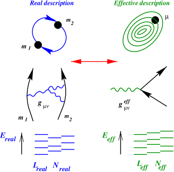
The resummation technique discussed in this section, the so-called effective-one-body (EOB) approach [22], was originally inspired by a similar approach introduced by Brézin, Itzykson and Zinn-Justin [26] to study electromagnetically interacting two bodies. The basic idea, illustrated in Fig. 2, is to map the real conservative two-body dynamics up to 2PN order (see below for the extension at 3PN order) onto an effective one-body problem, where a test particle of mass , with , the black-hole masses and , moves in some effective background metric . This mapping has been worked out within the Hamilton-Jacobi formalism, by imposing that whereas the action variables of the real and effective description coincide, i.e. , , where denotes the total angular momentum, and the radial action variable, the energy axis is allowed to change, , where is a generic function. By applying the above rules defining the mapping, it was found that as long as radiation-reaction effects are not taken into account, the effective metric is just a deformation of the Schwarzschild metric, with deformation parameter .
The effective metric reads [22]:
| (6) |
More importantly the reduction to the one-body dynamics provides the improved real Hamiltonian
| (7) |
where are the ADM coordinates used in the real description. The effective coordinates can be related to by a (generalized) canonical transformation given at 2PN order in Ref. [22] and at 3PN order in Ref. [24]. The effective Hamiltonian reads:
| (8) |
We refer to the real Hamiltonian (7) as improved real Hamiltonian because being a (partial) PN resummation of the original badly convergent real Hamiltonian , it should better capture the nonperturbative effects of the final stage of the black-hole motion. Remarkably, the mapping between the real and the effective Hamiltonians in Eq. (7) coincides with the mapping obtained in Ref. [26] in the context of quantum electrodynamics, where these authors mapped the one-body relativistic Balmer formula onto the two-body energy formula.
The EOB approach was then extended at 3PN order in Ref. [24]. The authors found that starting from the 3PN level there are more equations to satisfy than the number of free parameters appearing in the energy-map and in the effective metric. Hence, they suggested the following two possibilities. At the price of modifying the coefficients of the effective metric at 1PN and 2PN levels, and the energy-map (7) as well, it is still possible at 3PN order to (uniquely) map the real two-body dynamics onto the dynamics of a test mass moving on a geodesic [see for detail Appendix A of Ref. [24]]. However, this solution looks quite complicated and, more importantly, it does not look very natural to wait to know the 3PN Hamiltonian to derive the matching at 1PN and 2PN levels. The authors then suggested to abandon the hypothesis (used at 2PN order [22]) that the effective test mass moves along a geodesic and introduced in the Hamilton-Jacobi equation (arbitrary) higher derivatives terms which provide enough coefficients to obtain the matching. Because of these terms the effective 3PN Hamiltonian is not uniquely fixed by the matching rules defined above; the general expression is given by Eq. (3.12) in Ref. [24]. It is interesting to note that also in the non-geodesic case the relation between the effective and real Hamiltonians is still given by Eq. (7).
|
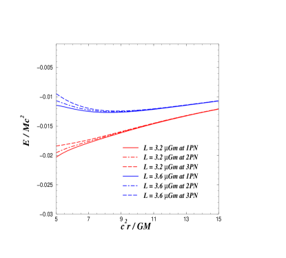 |
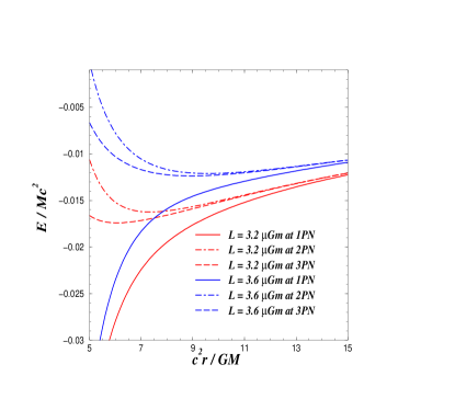
To have a qualitative understanding of the way the EOB can accelerate the PN convergence, we compare in Figs. 3 the PN-expanded binding energy (on the left panel) to the EOB-resummed binding energy (on the right panel) versus the radial separation, for circular orbits, in the equal-mass case, for two choices of the angular momentum and at different PN orders. [To obtain the plots we used the 3PN-expanded and EOB-resummed Hamiltonians given by Eqs. (3.12) and (4.27) of Ref. [24] with [9] and . We also used the (generalized) canonical transformation between the ADM and the “effective” coordinates given by Eqs. (4.29)–(4.36) of Ref. [24].]
Note that the PN-expanded energy oscillates at the various PN orders while the EOB energy has a monotonic behaviour. The fractional difference between the PN-expanded and EOB binding energies is, e.g., for , (2PN order) and (3PN order) at and (2PN order) and (3PN oder) at .
An interesting nonperturbative information of binary black hole systems is the presence of the ISCO defined as the solution of the equations . In the test mass limit (Schwarzschild metric) the ISCO exists and the nonrelativistic energy associated to it is . If we consider the PN-expanded real Hamiltonian [Eq. (4.27) of Ref. [24]] in the test mass limit and look for the ISCO, we find that at 1PN order , at 2PN order the ISCO does not exist, while at 3PN order . On the other hand, because by definition the EOB converges in the test mass limit to the Schwarzschild case, it automatically provides the correct ISCO. Thus, in the same way as Padé approximants, the EOB resummation method, provides by construction the right prediction in the test mass limit. Although we cannot prove that in the comparable-mass case the EOB approach is converging to the right limit, however, we can certainly say that it shows reasonable stability in the predictions at 1PN, 2PN and 3PN orders.
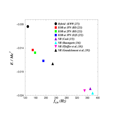
In Fig. 4 we summarize the binding energy at the ISCO predicted by various post-Newtonian [27, 22, 24] and numerical relativity calculations [15, 16, 17, 18]. The equal-mass ISCO binding energies predicted by the EOB approach at various PN orders are: (1PN order), (2PN order) and (3PN order). Note that the fractional difference from 1PN to 2PN order is and it increases to from 2PN to 3PN order. Figure 4 shows that except the very recent result of Ref. [18], which is much closer (probably due to their definition of the binary orbital frequency) to the PN estimates than the numerical relativity predictions, the PN and numerical relativity results [15, 16, 17] differ very much.
2.3 Beyond the adiabatic approximation: transition inspiral to plunge
Let us now introduce radiation-reaction effects. As discussed in Sec. 2.2.1, Padé approximants [21] give a good estimate of the energy-loss rate along circular orbits up to 2.5 PN order. In Ref. [23] this resummation method was combined with the EOB approach, and the authors deduced a system of ordinary differential equations which describe the late dynamical evolution of a binary–black-hole system. In spherical coordinates , their relevant equations are [23]:
| (9) |
Differently from Eqs. (2), the above equations go beyond the adiabatic approximation (at least for what concerns the conservative part of the dynamics) and can be analytically or numerically solved to study the transition between the adiabatic inspiral and the plunge.
Let us discuss briefly the main features of this transition in the two extreme limits and [see Ref. [23] for more details]. The case refers to binary–black-hole systems in which a very small black hole spirals around a supermassive black hole. They are typical GW sources for the Laser Interferometer Space Antenna (LISA). In this case, it was found [22, 28] that the transition from adiabatic inspiral to plunge is sharply localized around the ISCO. Ori and Thorne [28] pointed out that likely LISA could observe the transition from inspiral to plunge with a signal-to-noise ratio of a few.
For equal-mass binaries (), the radiation damping effects are important in an extended region on the order of above the naive (Schwarzschild) ISCO . The transition from inspiral to plunge is rather blurred and the dephasing between the full and the adiabatic waveform becomes visible somewhat before the naive ISCO. The plunge part of the exact waveform looks like a continuation of the inspiral part because the orbital motion remains quasi-circular throughout the plunge.
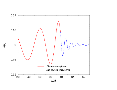
Figure 5 shows the plunge, merger and ring-down part of the waveform [23] for equal-mass binary. The ringdown waveform contains only the mode that is damped more slowly, , [3], at frequency Hz, where is the mass of the final black hole formed. The dimensionless rotation parameter is , where we denoted the angular momentum of the final Kerr black hole by . The energy emitted during the plunge is of , with a comparable energy loss of during the ring-down phase [30]. This gives a total energy released of of to be contrasted with the much larger value of recently estimated in Ref. [20].
Recently Damour, Iyer and Sathyaprakash [29] investigated the consequences of the EOB waveform for LIGO/VIRGO data analysis. They derived that the GW radiation coming from the plunge and merger can significantly enhance the signal-to-noise ratio for binaries of total mass . They found that the signal-to-noise ratio reaches the maximum value of for at . Previous estimations using maximally spinning binaries found that the merger dominates on inspiral. For example Flanagan and Hughes [31] predicted that the energy released during the plunge is while during the ring-down phase and the signal-to-noise ratio reaches the maximum value of for at .
3 Open issues
3.1 Spinning binary black holes
The theoretical prediction of GWs from comparable-mass binaries is not only affected by the failure of the PN-expansion, but also by spin effects. Various studies [32, 33] estimated that if the binary’s holes carry a spin, the evolution in time of the GW phase will be significantly affected by it – for example the spin can introduce modulations and irregularities in the gravitational waveforms. These features can become quite “dramatic” as long as the two spins are big and not aligned or antialigned with the orbital angular momentum.
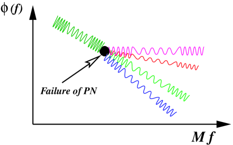
To give a rough idea of the effects we are alluding to and that we are currently investigating [38], we sketch in Fig. 6 the Fourier-domain phase of the GW signal versus frequency for various approaches, including possible modulations due to spin effects. The various methods give the same prediction for the Fourier-domain phase up to the frequency where the PN series fails – for example for , , while for , [2], which are well inside the LIGO/VIRGO band.
More recently, Levin [34] claimed that because of spin effects the two-body dynamics could be affected by chaos, or more in general the dynamics, and as a consequence the gravitational waveform, could depend strongly on the initial conditions. However, Schnittman and Rasio reanalysed this issue in Ref. [35]. By calculating the divergence of nearby trajectories for a broad sample of initial conditions they concluded that the divergent time is much greater that the inspiral time. So even if chaos were present it should not affect the detection of inspiral waveforms with LIGO/VIRGO.
To tackle these delicate issues it would be desirable to extend the resummation methods discussed above to the case of spinning binaries. To this respect we notice that the Padé resummation method has been recently extended to the gravitational flux function including spin-orbit and spin-spin effects [37]. Moreover, on the line of the EOB appoach, Damour [36] has recently mapped the conservative dynamics of two spinning black holes into the one of a test particle moving in an external -deformed Kerr metric. It will be very important to complete Damour’s analysis by including radiation reaction effects and describe the late nonadiabatic dynamics of spinning black hole binaries.
3.2 Possible strategy for not missing the GW signal from comparable-mass binary black holes
In sections 2.2.1 and 2.2.2 we discussed the best theoretical gravitational waveforms currently available. These waveforms should certainly be used in detecting and extracting physical parameters (masses and spins) for GWs emitted by neutron-star binaries and neutron-star/ black hole binaries. On the other hand the direct application of these templates to detect GWs from comparable-mass black-hole binaries is less straightforward. Indeed, the approaches analysed in sections 2.2.1 and 2.2.2 are inevitably affected by approximations and assumptions, introduced to overtake the fact that the two-body problem is known only up to a certain PN order. It would be important for detection purposes to quantify such uncertainties and take them into account when building the best theoretical GW templates. If not, the risk is to miss the GW signal. A possibility [39] is to deform and expand (e.g., by introducing new parameters), the template family generated by the resummation method having better PN convergent properties, in such a way that the new (higher-dimensional) template space could (i) include, or at least be not very far, from all the other approaches characterized by worse PN convergent properties and (ii) describe signals (hopefully the real GW signal!) whose functional form cannot be described by any of the original template families. To reach this goal the ideas underlying the Fast Chirp Transform technique, recently proposed in Ref. [40], deserves attention. Moreover, for comparable-mass binaries the inclusion of spin effects and the enlargement of the template space, hopefully, should not make the total number of templates huge, because the number of cycles expected in the LIGO/VIRGO band for nonspinning binaries is already rather small . [The situation would be different for neutron star or neutron-star/black hole binaries for which in the nospinning case we expect a number of cycles on the order of .]
The new template space [39] could be used for on-line search. When an acceptable signal-to-noise ratio is found, say , then the output signal could be re-analysed by templates provided, e.g., by the PN Taylor-expanded, Padé approximant and EOB methods, to (i) determine which approach better describe the real signal and (ii) extract the binary’s parameters, as the masses and the spins.
References
References
- [1] Abramovici A, Althouse W E, Drever R W P, Gursel Y, Kawamura S, Raab F J, Shoemaker D, Sievers L, Spero R E, Thorne K S, Vogt R E, Weiss R, Whitcomb S E and Zucker M E 1992 Science 256 325; Caron B et al. 1997 Class. Quantum Grav. 14 1461; Lück H et al. 1997 Class. Quantum Grav. 14 1471; Ando M et al. 2001 Preprint astro-ph/0105473.
- [2] Brady P R, Creighton J D E and Thorne K S 1998 Phys. Rev. D 58 061501.
- [3] Chandrasekhar S and Detweiler S 1975 Proc. R. Soc. Lond. A 344 441.
- [4] Lipunov V M, Postnov K A and Prokhorov M E 1997 New Astron. 2 43.
- [5] Thorne K S “The scientific case for mature LIGO interferometers,” (LIGO Document Number P000024-00-R, www.ligo.caltech.edu/docs/P/P000024-00.pdf).
- [6] Portegies Zwart S F and McMillan S L (2000) Astrophys. J. 528 L17.
- [7] Damour T and Deruelle N 1981 Phys. Lett. 87A 81; Damour T 1982 C.R. Seances Acad. Sci. Ser. 2 294 1355.
- [8] Jaranowski P and Schäfer G 1998 Phys. Rev. D 57 7274; ibid. 1999 Phys. Rev. D 60 124003; Damour T, Jaranowski P and Schäfer G 2000 Phys. Rev. D 62 044024; ibid. Phys. Rev. D 62 021501 (R); ibid. 2001 Phys. Rev. D 63 044021.
- [9] Damour T, Jaranowski P and Schäfer G 2001 Phys. Lett. B 513 147.
- [10] Blanchet L and Faye G 2000 Phys. Lett. A271 58; ibid. 2001 J. Math. Phys. 42 4391; ibid. 2000 Phys. Rev. D 63 062005; de Andrade V C, Blanchet L and Faye G 2001 Class. Quant. Grav. 18 753.
- [11] Wagoner R V and Will C M 1976 Astrophys. J. 210 764.
- [12] Blanchet L, Damour T, Iyer B R, Will C M and Wiseman A G 1995 Phys. Rev. Lett. 74 3515; Blanchet L, Damour T and Iyer B R 1995 Phys. Rev. D 51 536; Will C M and Wiseman A G 1996 Phys. Rev. D 54 4813.
- [13] Blanchet L 1996 Phys. Rev. D 54 1417; Blanchet L 1998 Class. Quantum Grav. 15 113.
- [14] Blanchet L, Faye G, Iyer B.R., Joguet B 2002 Phys. Rev. D 65 061501; Blanchet L, Iyer B R and Joguet B 2002 Phys. Rev. D 65 064005.
- [15] Cook G B 1994 Phys. Rev. D 50 5025.
- [16] Baumgarte T W 2000 Phys. Rev. D 62 024018.
- [17] Pfeiffer HP, Teukolsky SA and Cook GB 2000 Phys. Rev. D 62 104018.
- [18] Gourgoulhon E, Grandclément P and Bonazzola S (2002) Phys. Rev. D 65 044020; Grandclément, Gourgoulhon E and Bonazzola S (2002) Phys. Rev. D 65 044021.
- [19] Alcubierre M, Brügmann B, Pollney D, Seidel E and Takahashi R 2001 Phys. Rev. D 64 061501; Kidder L.E., Scheel M.A. and Teukolsky S.A. 2001 Phys. Rev. D 64 064017.
- [20] Baker J, Brügmann B, Campanelli M, Lousto C O and Takahashi R 2001 Phys. Rev. Lett. 87 121103.
- [21] Damour T, Iyer B R and Sathyaprakash B S 1998 Phys. Rev. D 57 885.
- [22] Buonanno A and Damour T 1999 Phys. Rev. D 59 084006.
- [23] Buonanno A and Damour T 2000 Phys. Rev. D 62 064015.
- [24] Damour T, Jaranowski P and Schäfer G 2000 Phys. Rev. D 62 084011.
- [25] Bender C M and Orszag S A, Advanced Mathematical Methods for Scientists and Engineers (McGraw Hill, Singapore, 1984).
- [26] Brézin E, Itzykson C and Zinn-Justin J 1970 Phys. Rev. D 1 2349.
- [27] Kidder L E, Will C M and Wiseman A G 1992 Class. Quantum Grav. 9 L127; ibid. 1993 Phys. Rev. D 47 3281.
- [28] Ori A and Thorne K S (2000) Phys. Rev. D 62 124022.
- [29] Damour T, Iyer B R and Sathyaprakash B S 2001 Phys. Rev. D 63 044023.
- [30] Buonanno A and Damour T, contributed paper to the IXth Marcel Grossmann Meeting (Rome, July 2000); 2000 Preprint gr-qc/0011052.
- [31] Flanagan E E and Hughes S A 1998 Phys. Rev. D 57 4535.
- [32] Kidder L E, Will C M and Wiseman A G 1993 Phys. Rev. D 47 4183 (R); Kidder L E 1995 Phys. Rev. D 52 821.
- [33] Apostolatos T A, Cutler C, Sussman G J and Thorne K S 1994 Phys. Rev. D 15 6274; Apostolatos T A 1996 Phys. Rev. D 54 2438.
- [34] Levin J 2000 Phys. Rev. Lett. 84 3515; and 2000 Preprint gr-qc/0010100.
- [35] Schnittman JD and Rasio F 2001 Phys. Rev. Lett. 87 121101.
- [36] Damour T 2001 Phys. Rev. D 64 124013.
- [37] Porter E and Sathyaprakash B S, in preparation.
- [38] Buonanno A, Chen Y, Chernoff D and Vallisneri M, work in progress.
- [39] Buonanno A, Chen Y and Vallisneri M, in preparation.
- [40] Jenet F A and Prince T 2000 Phys. Rev. D 62 122001.
- [41] Blanchet L 2001 Preprint gr-qc/0112056.