The back reaction and the effective Einstein’s equation for the Universe with ideal fluid cosmological perturbations

Abstract

We investigate the back reaction of cosmological perturbations on the evolution of the Universe using the renormalization group method. Starting from the second order perturbed Einstein’s equation, we renormalize a scale factor of the Universe and derive the evolution equation for the effective scale factor which includes back reaction due to inhomogeneities of the Universe. The resulting equation has the same form as the standard Friedman-Robertson-Walker equation with the effective energy density and pressure which represent the back reaction effect.

I introduction

Owing to the nonlinear nature of Einstein’s equation, fluctuations of the metric affect the evolution of the background space time. In cosmology, this effect is expected to be important when we consider the evolution of large scale nonlinear structures and the evolution of the early Universe. This is cosmological the back reaction problem and has been studied by several authorsIssacson (1968); Futamase (1989, 1996); Russ et al. (1997); Boersma (1998); Mukhanov et al. (1997); Abramo et al. (1997); Abramo (1997, 1999); Nambu (2000, 2001).

One of the main difficulty in the cosmological back reaction problem is connected with the gauge freedom of perturbation variables. The back reaction effect appears from the second order quantities in a perturbation expansion and we must use the second order gauge invariant quantities to avoid the gauge ambiguity of the back reaction problem. Abramo and co-workersMukhanov et al. (1997); Abramo et al. (1997); Abramo (1997, 1999) derived the gauge-invariant effective energy momentum tensor of cosmological perturbations and applied their formalism to the inflationary universe. They discussed the effect of the inhomogeneity on the background Friedman-Robertson-Walker (FRW) universe, but did not derive solutions of an effective scale factor for the FRW universe with the back reaction.

In our previous papersNambu (2000, 2001), the renormalization group methodChen et al. (1996); Kunihiro (1995); Goto et al. (1999); Nambu and Yamaguchi (1999) was applied to the cosmological back reaction problem. We start from the following perturbation expansion of the metric

$$g_{ab}=\overset{(0)}{g}_{ab}+\overset{(1)}{g}_{ab}+\overset{(2)}{g}_{ab}+\cdots,$$ (1)

where $\overset{(0)}{g}_{ab}$ is the background FRW metric and represents a homogeneous and isotropic space. $\overset{(1)}{g}_{ab}$ is the metric of the first order linear perturbation with $\langle\overset{(1)}{g}_{ab}\rangle=0$ where $\langle\cdots\rangle$ means the spatial average with respect to the background FRW metric. $\overset{(2)}{g}_{ab}$ is the second order metric and this part contains nonlinear effects caused by the first order linear perturbation. This nonlinearity produces homogeneous and isotropic zero modes as part of the second order metric. That is,

$$\langle\overset{(2)}{g}_{ab}\rangle\neq 0.$$ (2)

As the zero mode part of the metric has the same symmetry as the background FRW universe, it must be interpreted as a part of FRW metric. Hence we redefine the background metric as follows:

$$\overset{(B)}{g}_{ab}=\overset{(0)}{g}_{ab}+\langle\overset{(2)}{g}_{ab}\rangle.$$ (3)

We used the renormalization group method to define the new background metric $\overset{(B)}{g}_{ab}$ which includes the back reaction effect. In previous papersNambu (2000, 2001), we first solved perturbation equations and obtained $\overset{(1)}{g}_{ab}$ and $\overset{(2)}{g}_{ab}$. Then the renormalized effective scale factor with the back reaction effect was obtained.

But it is more convenient to obtain the renormalized Einstein’s equation for the zero mode variables from the first to investigate the back reaction effect. This is equivalent to average Einstein’s equation and derive the evolution equation for the effective FRW universe with the back reaction effect. In this paper, we apply the renormalization group method directly to the perturbed Einstein’s equation. We does not use an explicit form of the first and the second order solutions of perturbations. All that we need is how constants of integration enter in the solution of perturbations.

The plan of this paper is as follows. In Sec. II, we introduce the gauge ready formalism of cosmological perturbations and derive the second order Einstein’s equation for gauge invariant variables. In Sec. III, the renormalization group method is applied to the zero mode part of the Einstein’s equation and the evolution equation for the renormalized scale factor is derived. In Sec. IV, we investigate the solution of the back reaction equation. Sec. V is devoted for summary and discussion. We use units in which $c=\hbar=8\pi G=1$ throughout the paper.

II the second order perturbation for the Universe with ideal fluid

To circumvent the gauge ambiguity of cosmological perturbations and to obtain a gauge independent interpretation of the cosmological back reaction problem, we must use gauge invariant description of cosmological perturbationsKodama and Sasaki (1984); Mukhanov et al. (1992). Abramo and co-workers obtained the gauge invariant effective energy-momentum tensor for cosmological perturbationsMukhanov et al. (1997); Abramo et al. (1997); Abramo (1997, 1999) which is quadratic with respect to the first order variables. To apply the renormalization group method to the back reaction problem, we must obtain the second order zero mode perturbation in a gauge invariant mannerNambu (2000, 2001). In this section, we introduce the gauge ready formalismHwang (1991) and derive the evolution equation for the second order zero mode perturbation which is invariant under the first order gauge transformation.

II.1 the gauge ready form of cosmological perturbations

We consider a spatially flat FRW universe with perfect fluid of which equation of state is given by $p=w\,\rho$, where $w$ is assumed to be constant. The background scale factor of the Universe and the energy density are given by

$$a(t)=C\,t^{\frac{2}{3(1+w)}},\quad\overset{(0)}{\rho}=\frac{c_{0}}{a^{3(1+w)}},$$ (4)

where $C$ and $c_{0}$ are constants of integration. The energy density of the fluid $\overset{(0)}{\rho}$ is obtained from the zeroth order of the following mass conservation equation

$$\left(\rho^{\frac{1}{1+w}}\sqrt{-g}\,u^{a}\right)_{,a}=0,$$ (5)

where $u^{a}$ is four velocity of the fluid. We restrict our attention only to the scalar type perturbation and the metric of the first order perturbation can be written as

$$\overset{(1)}{g}_{ab}=\left(\begin{array}[]{ll}-2\phi&a(t)B_{,i}\\ a(t)B_{,i}&a^{2}(t)\left[(1-2\psi)\,\delta_{ij}+2E_{,ij}\right]\end{array}\right).$$ (6)

Let us consider the infinitesimal coordinate transformation

$$x^{\prime}{}^{0}=x^{0}+\xi^{0},\quad x^{\prime}{}^{i}=x^{i}+\frac{1}{a^{2}}\delta^{ij}\xi_{,j}$$ (7)

Under this transformation, the perturbation variables receive the following gauge transformations:

$$\phi^{\prime}=\phi-\dot{\xi}{}^{0}, B^{\prime}=B-a\left(\frac{\xi}{a^{2}}\right)^{\dot{}}+\frac{\xi^{0}}{a},$$

$$\psi^{\prime}=\psi+H\xi^{0}, E^{\prime}=E-\frac{\xi}{a^{2}}.$$ (8)

The comoving three velocity $v_{i}=v_{,i}$ of the fluid transforms as

$$v^{\prime}=v+a^{2}\left(\frac{\xi}{a^{2}}\right)^{\dot{}},$$ (9)

and the velocity potential defined by $\chi\equiv v+aB$ transforms as

$$\chi^{\prime}=\chi+\xi^{0}.$$ (10)

From these transformations, we can make the following gauge invariant combination of perturbation variables:

$$\Phi\equiv\phi+\left[a(B-a\dot{E})\right]^{\dot{}}, \Psi\equiv\psi-aH(B-a\dot{E}),$$

$$X\equiv\chi-a(B-a\dot{E}), \mathcal{R}\equiv\psi-H\chi.$$ (11)

Now the vector

$$\xi^{\mu}_{\text{C}}\equiv\left(-\chi,~{}\delta^{ij}E_{,j}\right)$$ (12)

transforms as four vector under the coordinate transformation. The gauge transformation induced by the coordinate transformation using the vector (12) is

$$\phi^{\prime}=\phi+\dot{\chi}=\Phi+\dot{X}, B^{\prime}=B-a\dot{E}-\frac{\chi}{a}=-\frac{X}{a},$$

$$E^{\prime}=E-E=0, \psi^{\prime}=\psi-H\chi=\mathcal{R},$$ (13)

$$\chi^{\prime}=\chi-\chi=0.$$

Hence in this gauge, each components of the metric correspond to the gauge invariant variables and a comoving gauge condition $\chi=0$ is satisfied. The choice of the vector (12) is not unique. The vector

$$\xi^{\mu}_{\text{L}}=\left(-a(B-a\dot{E}),~{}\delta^{ij}E_{,j}\right)$$ (14)

also transforms as a four vector and the gauge transformation using this vector is

$$\phi^{\prime}=\phi+\left[a(B-a\dot{E})\right]^{\dot{}}=\Phi, B^{\prime}=0, E^{\prime}=0,$$ (15)

$$\psi^{\prime}=\psi-aH(B-a\dot{E})=\Psi, \chi^{\prime}=\chi-a(B-a\dot{E})=X.$$ (16)

This gauge corresponds to the longitudinal gauge and components of the metric coincide with gauge invariant variables $\Phi$ and $\Psi$. This gauge is often used to investigate cosmological perturbationsMukhanov et al. (1992), and Abramo and co-workerMukhanov et al. (1997); Abramo et al. (1997); Abramo (1997, 1999) also used this gauge to evaluate the gauge invariant energy momentum tensor of cosmological perturbations. But for the purpose of the back reaction problem, this gauge is not suitable because the contribution of long wavelength limit mode of the perturbations to the effective energy momentum tensor does not vanish automaticallyNambu (2001). The perturbation of which wavelength is infinite cannot be distinguished from the background and has nothing to do with the back reaction effect. But in the longitudinal gauge, we have contribution of the long wavelength limit perturbation to the second order quantities. We must subtract this to obtain correct back reaction effect. On the other hand, in comoving gauge, the second order perturbation becomes zero in the long wavelength limit. In this paper, therefore, we adopt the gauge ready form in the comoving gauge to investigate the back reaction problem.

To simplify the calculation, we choose $B=0$ and the metric up to the second order in the gauge (13) is given by

$$ds^{2}=-(1+2\phi+2\phi_{2})\,dt^{2}-2a^{2}\dot{E}_{,i}\,dx^{i}dt+a^{2}(t)(1-2\psi-2\psi_{2})\,d\boldsymbol{x}^{2}.$$ (17)

As the each component of the first order metric perturbation corresponds to the gauge invariant variable in this gauge, the second order zero mode variables $\phi_{2}$ and $\psi_{2}$ determined by the first order quantities are also invariant under the first order gauge transformation up to the second order.

Using the metric (17) with the comoving condition $\chi=0$, the first order Einstein equations are

$$\frac{1}{a^{2}}\nabla^{2}\psi+H\nabla^{2}\dot{E}=\frac{1}{2}\,\overset{(1)}{\rho},$$ (18a)

$$\dot{\psi}+H\phi=0,$$ (18b)

$$\ddot{\psi}+3H\dot{\psi}+H\dot{\phi}-3wH^{2}\phi=\frac{w}{2}\,\overset{(1)}{\rho},$$ (18c)

$$\ddot{E}+3H\dot{E}+\frac{1}{a^{2}}(\psi-\phi)=0.$$ (18d)

We can obtain the following evolution equation for the spatial curvature perturbation $\psi$

$$\ddot{\psi}+3H\dot{\psi}-\frac{w}{a^{2}}\nabla^{2}\psi=0.$$ (19)

II.2 the evolution equations for the second order zero mode perturbation

The second order Einstein equations for the zero mode variables $\phi_{2}$ and $\psi_{2}$ are

$$6H(\dot{\psi}_{2}+H\phi_{2})=-\langle\overset{(2)}{G}{}^{0}{}_{0}(\overset{(1)}{g})\rangle-\overset{(2)}{\rho},$$ (20a)

$$2[\ddot{\psi}_{2}+H(3\dot{\psi}_{2}+\dot{\phi}_{2})-3H^{2}w\phi_{2}]=-\frac{1}{3}\langle\overset{(2)}{G}{}^{i}{}_{i}(\overset{(1)}{g})\rangle+w\,\overset{(2)}{\rho},$$ (20b)

where

$$\langle\overset{(2)}{G}{}^{0}{}_{0}(\overset{(1)}{g})\rangle=\Biggl{\langle}-3\dot{\psi}^{2}+12H\psi\dot{\psi}-\frac{5}{a^{2}}\psi\nabla^{2}\psi-6H\psi\nabla^{2}\dot{E}\\ -3H^{2}a^{2}\dot{E}\nabla^{2}\dot{E}-2H\phi\left(-\nabla^{2}\dot{E}+6\dot{\psi}\right)-12H^{2}\phi^{2}\Biggr{\rangle},$$ (21)

$$\langle\overset{(2)}{G}{}^{i}{}_{j}(\overset{(1)}{g})\rangle=\Biggl{\langle}-\frac{5}{a^{2}}\psi\nabla^{2}\psi+\dot{\psi}^{2}+4\psi(\ddot{\psi}+3H\dot{\psi})-2\nabla^{2}\dot{E}\left(3H\psi+\frac{2}{3}\dot{\psi}\right)\\ -2\psi\nabla^{2}\ddot{E}-2a^{2}H\dot{E}\nabla^{2}\ddot{E}-(2\dot{H}+5H^{2})a^{2}\dot{E}\nabla^{2}\dot{E}+\frac{2}{3}\dot{E}\nabla^{2}\dot{\phi}-2\dot{\phi}\dot{\psi}\\ -4\phi\left(\ddot{\psi}+3H\dot{\psi}-\frac{1}{2a^{2}}\nabla^{2}\psi-\frac{1}{3}\left(\nabla^{2}\ddot{E}+2H\nabla^{2}\dot{E}\right)+2H\dot{\phi}\right)\\ -\frac{2}{3a^{2}}\phi\nabla^{2}\phi-4\phi^{2}\left(3H^{2}+2\dot{H}\right)\Biggr{\rangle}\,\delta{}^{i}{}_{j}.$$ (22)

Eq.(20a) is a time-time component and Eq.(20b) is a space-space component of the spatially averaged Einstein’s equation $\langle G^{a}{}_{b}\rangle=\langle T^{a}{}_{b}\rangle$. The spatial average is defined by

$$\langle A\rangle=\frac{1}{V}\int d^{3}x\,A,$$

where $V$ is the volume of a sufficiently large compact domain and periodic boundary conditions for perturbations are assumed. The second order energy density $\overset{(2)}{\rho}$ is determined by the mass conservation (5) and given by

$$\overset{(2)}{\rho}=(1+w)\,\overset{(0)}{\rho}\,(3\psi_{2}-\phi_{2})+3\langle\psi\,\overset{(1)}{\rho}\rangle+\frac{w}{2(1+w)}\frac{\langle\overset{(1)}{\rho}{}^{2}\rangle}{\overset{(0)}{\rho}}+c_{2}(1+w)\,\overset{(0)}{\rho},$$ (23)

where $c_{2}$ is a constant.

III the renormalization and the effective Einstein’s equation

In this section, we derive the effective Einstein’s equation which describes the evolution of the effective FRW universe with the back reaction effect using the renormalization group method. The spatially averaged Einstein’s equation up to the second order is

$$-3H^{2}+\overset{(0)}{\rho}+6H(\dot{\psi}_{2}+H\phi_{2})+(1+w)\,\overset{(0)}{\rho}(3\psi_{2}-\phi_{2}+c_{2})=-\rho_{\text{BR}},$$ (24a)

$$-2\dot{H}-3H^{2}-w\,\overset{(0)}{\rho}+2\left[\ddot{\psi}_{2}+H(3\dot{\psi}_{2}+\dot{\phi}_{2})-3H^{2}w\phi_{2}\right]$$

$$\qquad\qquad\qquad\qquad\qquad\qquad-w(1+w)\overset{(0)}{\rho}(3\psi_{2}-\phi_{2}+c_{2})=p_{\text{BR}},$$ (24b)

where

$$\rho_{\text{BR}}\equiv\langle\overset{(2)}{G}{}^{0}{}_{0}(\overset{(1)}{g})\rangle+3\langle\psi\overset{(1)}{\rho}\rangle+\frac{w}{2(1+w)}\frac{\langle\overset{(1)}{\rho}{}^{2}\rangle}{\overset{(0)}{\rho}},$$ (25a)

$$p_{\text{BR}}\equiv-\frac{1}{3}\,\langle\overset{(2)}{G}{}^{i}{}_{i}(\overset{(1)}{g})\rangle+3w\langle\psi\overset{(1)}{\rho}\rangle+\frac{w^{2}}{2(1+w)}\frac{\langle\overset{(1)}{\rho}{}^{2}\rangle}{\overset{(0)}{\rho}}.$$ (25b)

By introducing a new time variable $d\tau\equiv(1+\phi_{2})\,dt$, the Einstein equations (24a) and (24b) become

$$-3H^{2}+6H\dot{\psi}_{2}+\overset{(0)}{\rho}\left[1+(1+w)(3\psi_{2}-\phi_{2}+c_{2})\right]=-\rho_{\text{BR}},$$ (26a)

$$-2\dot{H}-3H^{2}+2\,(\ddot{\psi}_{2}+3H\dot{\psi}_{2})-w\overset{(0)}{\rho}\left[1+(1+w)(3\psi_{2}-\phi_{2}+c_{2})\right]=p_{\text{BR}},$$ (26b)

where $\dot{}=\frac{d}{d\tau}$.

The spatially averaged line element up to the second order perturbation is

$$\langle ds^{2}\rangle=-d\tau^{2}+a^{2}(\tau)\left[1-2\,\psi_{2}(\tau)+2\psi_{2}(\tau_{0})\right]\,d\boldsymbol{x}^{2},\quad a(\tau)=C\tau^{\frac{2}{3(1+w)}},$$ (27)

where $\tau_{0}$ is a time at which the initial condition is set, and it is always possible to write the zero mode metric as Eq.(27) by choosing a constant of integration $c_{2}$ contained in $\overset{(2)}{\rho}$ as $c_{2}=-3\,\psi_{2}(\tau_{0})$. From this form of the line element, we can observe that the effective scale factor for the FRW universe is

$$a_{\text{eff}}(\tau)=\tau^{\frac{2}{3(1+w)}}\,C\,\left[1-\psi_{2}(\tau)+\psi_{2}(\tau_{0})\right].$$ (28)

We regard the second order perturbation $\psi_{2}$ as a secular term and apply the renormalization group methodChen et al. (1996); Kunihiro (1995); Goto et al. (1999); Nambu and Yamaguchi (1999) to absorb it to the zeroth order constant of integration $C$. We redefine the zeroth order integration constant $C$ as

$$C=C(\mu)+\delta C(\mu;\tau_{0}),$$

where $\mu$ is a renormalization point and $\delta C$ is a counterterm which absorbs the secular divergence of the solution. We assume that $\delta C$ is the second order quantity. The effective scale factor (28) up to the second order of the perturbation can be written

$$a_{\text{eff}}(\tau) =\tau^{\frac{2}{3(1+w)}}\,(C(\mu)+\delta C(\mu;\tau_{0}))(1-\psi_{2}(\tau)+\psi_{2}(\mu)-\psi_{2}(\mu)+\psi_{2}(\tau_{0}))$$

$$=\tau^{\frac{2}{3(1+w)}}\,C(\mu)(1-\psi_{2}(\tau)+\psi_{2}(\mu)),$$

where we have chosen the counterterm $\delta C$ so as to absorb the $(\psi_{2}(\mu)-\psi_{2}(\tau_{0}))$-dependent term:

$$\delta C(\mu;\tau_{0})+C(\mu)(-\psi_{2}(\mu)+\psi_{2}(\tau_{0}))=0.$$ (29)

This defines the renormalization transformation

$$\mathcal{R}_{\mu-\tau_{0}}:C(\tau_{0})\longmapsto C(\mu)=C(\tau_{0})-C(\mu)\,\left[\psi_{2}(\mu)-\psi_{2}(\tau_{0})\right],$$ (30)

and this transformation forms Lie group. The renormalization group equation is obtained by differentiating the both side of the transformation with respect to $\mu$ and setting $\tau_{0}=\mu$:

$$\frac{dC(\mu)}{d\mu}=-C(\mu)\frac{d\psi_{2}(\mu)}{d\mu},$$ (31)

and its solution is

$$C(\mu)=C(\tau_{0})\,e^{-\psi_{2}(\mu)+\psi_{2}(\tau_{0})}.$$ (32)

By equating $\mu=\tau$ in the effective scale factor, the renormalized scale factor is given by

$$a_{R}(\tau)=\tau^{\frac{2}{3(1+w)}}\,C(\tau)=a(\tau)\,e^{-\psi_{2}(\tau)+\psi_{2}(\tau_{0})}.$$ (33)

By substituting the relation $a(\tau)=a_{R}(\tau)e^{\psi_{2}(\tau)-\psi_{2}(\tau_{0})}$ into (26a) and (26b), and keeping terms up to the second order of the perturbation, we obtain the following equations for the renormalized scale factor $a_{R}$:

$$-3H^{2}+\rho_{0}=-\rho_{\text{BR}},$$ (34a)

$$-2\dot{H}-3H^{2}-w\rho_{0}=p_{\text{BR}},$$ (34b)

where $H=\frac{\dot{a}_{R}}{a_{R}}$ and

$$\rho_{0}\equiv\left[1-(1+w)\phi_{2}\right]\frac{c_{0}}{(a_{R})^{{3(1+w)}}}=\frac{c_{0}}{\left[(1+\phi_{2})\,a_{R}^{3}\right]^{1+w}}.$$

(34a) and (34b) are the main result of this paper. The second order curvature variable $\psi_{2}$ disappears in the evolution equation by the procedure of the renormalization. The second order lapse function $\phi_{2}$ remains in the expression $\rho_{0}$, but this variable corresponds to the second order gauge freedom to parameterize time and we can freely choose the form of this function. Eqs.(34a) and (34b) have the same form as the standard FRW equations. On the right-hand side, the back reaction effect appears as source terms $\rho_{\text{BR}}$ and $p_{\text{BR}}$, and their explicit form is determined by solving the first order perturbation.

IV solutions of the effective Einstein’s equation

In this section, we solve the effective Einstein equations (34a) and (34b), and investigate how the inhomogeneity affects the expansion of the Universe. By eliminating the variable $\rho_{0}$, we have

$$-2\dot{H}-3(1+w)H^{2}=w\rho_{\text{BR}}+p_{\text{BR}}.$$ (35)

For $w\neq-1$, by using a new variable $x\equiv\left(a_{R}\right){}^{\frac{3}{2}(1+w)}$,

$$\ddot{x}=-\frac{3}{4}(1+w)(w\rho_{\text{BR}}+p_{\text{BR}})\,x.$$ (36)

We solve this equation for various value of $w$.

IV.1 vacuum energy case $w=-1$

The universe expands exponentially $a\propto e^{Ht},H=\text{const.}$, and we must treat this case separately. In this case, the perturbation of energy density is zero and the effective Einstein’s equation becomes

$$-3H^{2}+\rho_{0}=-\rho_{\text{BR}}=-\langle\overset{(2)}{G}{}^{0}{}_{0}(\overset{(1)}{g})\rangle,$$

$$-2\dot{H}-3H^{2}+\rho_{0}=p_{\text{BR}}=-\frac{1}{3}\langle\overset{(2)}{G}{}^{i}{}_{i}(\overset{(1)}{g})\rangle,\quad\rho_{0}=\text{const.}$$ (37)

For long wavelength perturbation $k\ll aH$, the first order growing mode solution is given by

$$\psi\approx\sum_{\boldsymbol{k}}C_{\boldsymbol{k}}e^{i\,\boldsymbol{k}\cdot\boldsymbol{x}},\quad\phi\approx 0,\quad\dot{E}\approx-\frac{1}{Ha^{2}}\sum_{\boldsymbol{k}}C_{\boldsymbol{k}}e^{i\,\boldsymbol{k}\cdot\boldsymbol{x}},$$

where $C_{\boldsymbol{k}}$ is a constant in time. The source terms of the effective Einstein’s equation are

$$\rho_{\text{BR}}\approx\frac{2}{a_{R}^{2}}\sum_{\boldsymbol{k}}k^{2}|C_{\boldsymbol{k}}|^{2},\quad p_{\text{BR}}\approx-\frac{2}{3a_{R}^{2}}\sum_{\boldsymbol{k}}k^{2}|C_{\boldsymbol{k}}|^{2}=-\frac{1}{3}\rho_{\text{BR}}.$$

This is equivalent to a negative spatial curvature term. For the slow roll inflationary phase driven by a scalar field, it was shown that the back reaction effect by the long wavelength perturbation is equivalent to positive spatial curvatureNambu (2001). For vacuum energy case, fluctuation of the energy density becomes identically zero and this leads to the different back reaction effect compared to the inflation with a scalar field.

For short wavelength mode $k\gg aH$, the first order curvature perturbation is given by

$$\psi\approx\sum_{\boldsymbol{k}}\frac{C_{\boldsymbol{k}}}{ka}\cosh\left(\frac{k}{aH}\right)e^{i\boldsymbol{k}\cdot\boldsymbol{x}}$$

and

$$\rho_{\text{BR}}\approx\frac{7}{2}\sum_{\boldsymbol{k}}\frac{|C_{\boldsymbol{k}}|^{2}}{a_{R}^{4}},\quad p_{\text{BR}}\approx\frac{7}{6}\sum_{\boldsymbol{k}}\frac{|C_{\boldsymbol{k}}|^{2}}{a_{R}^{4}}.$$

The back reaction effect is equivalent to a radiation fluid and this result is the same as the inflation with a scalar field.

IV.2 dust case $w=0$

The exact solution of the first order growing mode is

$$\psi=\sum_{\boldsymbol{k}}C_{\boldsymbol{k}}\,e^{i\,\boldsymbol{k}\cdot\boldsymbol{x}},\quad\phi=0,\quad\dot{E}=-\frac{3}{5}\tau^{-1/3}\sum_{\boldsymbol{k}}C_{\boldsymbol{k}}\,e^{i\,\boldsymbol{k}\cdot\boldsymbol{x}},\quad\overset{(1)}{\rho}=-\frac{6}{5}\sum_{\boldsymbol{k}}\frac{k^{2}}{a{}^{2}}\,C_{\boldsymbol{k}}\,e^{i\,\boldsymbol{k}\cdot\boldsymbol{x}},$$ (38)

where $C_{\boldsymbol{k}}$ is a constant in time. Using this solution, the source terms of the effective Einstein equation are

$$\rho_{\text{BR}}=-\frac{13}{25}\sum_{\boldsymbol{k}}\frac{k^{2}\,|C_{\boldsymbol{k}}|^{2}}{a_{R}{}^{2}},\quad p_{\text{BR}}=\frac{13}{3\cdot 25}\sum_{\boldsymbol{k}}\frac{k^{2}\,|C_{\boldsymbol{k}}|^{2}}{a_{R}{}^{2}}=-\frac{1}{3}\rho_{\text{BR}}.$$ (39)

This is the same equation of state as a positive spatial curvature term. The equation (36) becomes

$$\ddot{x}=-\frac{3A}{4}\,x^{-1/3},\quad A=\frac{13}{3\cdot 25}\sum_{\boldsymbol{k}}k^{2}|C_{\boldsymbol{k}}|^{2},$$ (40)

and the solution is

$$a_{R}=\frac{4E}{9A}(1-\cos\eta),\quad t=\frac{4E}{9A^{3/2}}(\eta-\sin\eta),$$ (41)

where $E$ is a constant of integration. This solution is the same as a closed FRW universe with dust. Therefore, the inhomogeneity works as a positive spatial curvature in the dust dominated universeRuss et al. (1997); Nambu (2000) and the Universe will recollapse.

IV.3 $w\neq 0$ case

For long wavelength perturbations $k\ll a\,H$, using the long wavelength expansion, the first order solution up to $O(k^{2})$ is given by

$$\psi\approx\sum_{\boldsymbol{k}}C_{\boldsymbol{k}}\,e^{i\,\boldsymbol{k}\cdot\boldsymbol{x}},\quad\phi\approx 0,\quad\dot{E}\approx-\frac{3(1+w)}{3w+5}\,\tau^{\frac{3w-1}{3(1+w)}}\,\sum_{\boldsymbol{k}}C_{\boldsymbol{k}}\,e^{i\,\boldsymbol{k}\cdot\boldsymbol{x}},$$

$$\overset{(1)}{\rho}\approx-\frac{6(1+w)}{3w+5}\sum_{\boldsymbol{k}}\frac{k^{2}}{a{}^{2}}\,C_{\boldsymbol{k}}\,e^{i\,\boldsymbol{k}\cdot\boldsymbol{x}},$$ (42)

and

$$\rho_{\text{BR}}\approx-\frac{9w^{2}+30w+13}{(3w+5)^{2}}\,\sum_{\boldsymbol{k}}\frac{k^{2}}{a_{R}{}^{2}}\,|C_{\boldsymbol{k}}|^{2},$$

$$p_{\text{BR}}\approx-\frac{162w^{3}+423w^{2}+276w-13}{3(3w+5)^{2}}\,\sum_{\boldsymbol{k}}\frac{k^{2}}{a_{R}{}^{2}}\,|C_{\boldsymbol{k}}|^{2}.$$ (43)

The effective Einstein equation (36) becomes

$$\ddot{x}=\frac{3}{4}(1+w)(wA-B)\,x^{\frac{3w-1}{3(w+1)}},$$ (44)

where

$$A=-\frac{9w^{2}+30w+13}{(3w+5)^{2}}\sum_{\boldsymbol{k}}k^{2}|C_{\boldsymbol{k}}|^{2},\quad B=-\frac{162w^{3}+423w^{2}+240w-13}{3(3w+5)^{2}}\sum_{\boldsymbol{k}}k^{2}|C_{\boldsymbol{k}}|^{2}.$$ (45)

By integrating the equation with respect to $\tau$, we obtain

$$\frac{\dot{x}^{2}}{2}+V_{\text{eff}}(x)=E,\quad V_{\text{eff}}=-\frac{3}{8}\frac{(w+1)^{2}(135w^{3}+333w^{2}+201w-13)}{(3w+1)(3w+5)^{2}}\sum_{\boldsymbol{k}}k^{2}|C_{\boldsymbol{k}}|^{2}\,x^{\frac{2(3w+1)}{3(w+1)}},$$ (46)

where $E$ is a constant of integration. If there is no inhomogeneity, $V_{\text{eff}}=0$ and the solution of the effective Einstein’s equation reduces to that of the background FRW solution. The condition $E>0$ is necessary to reproduce the background the solution when the inhomogeneity vanishes. We can obtain qualitative behavior of the effective scale factor by observing the shape of the effective potential $V_{\text{eff}}(x)$ (FIG. 1).

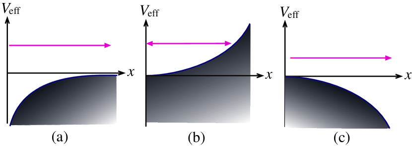
Figure 1: Effective potentials for the long wavelength perturbations. (a) is for $-1<w<-1/3$, (b) is for $-1/3<w<w_{*}$ and (c) is for $w_{*}<w<1$. For $-1<w<w_{*}$, inhomogeneity reduces the expansion rate of the Universe. For $w_{*}<w<1$, inhomogeneity enhances the expansion of the Universe. For $w=w_{*}$, there is no back reaction effect.

We can summarize the back reaction effect of the long wavelength perturbation on the expansion of the Universe as follows:

• $-1<w<-1/3$ : the expansion of the Universe is accelerating. The inhomogeneity reduces the expansion rate.

• $w=-1/3$ : $V_{\text{eff}}\propto\ln x$. The expansion of the Universe is decelerating. The inhomogeneity reduces the expansion rate and the universe will recollapse due to the back reaction effect.

• $-1/3<w<w_{*}$ : $w_{*}$ is a real root of the equation $135w^{3}+333w^{2}+201w-13=0$ and $w_{*}\approx 0.06$. The expansion of the Universe is decelerating. The inhomogeneity reduces the expansion rate and the universe will recollapse.

• $w=w_{*}$ : $V_{\text{eff}}=0$ and there is no back reaction.

• $w_{*}<w<1$ : the expansion of the Universe is decelerating. The inhomogeneity increases the expansion rate.

For short wavelength perturbations $k\gg a\,H$, WKB type solution for the curvature perturbation $\psi$ is given by

$$\psi\approx\begin{cases}\displaystyle\sum_{\boldsymbol{k}}\frac{C_{\boldsymbol{k}}}{k\sqrt{w}\,a}\cos\left(k\sqrt{w}\int\frac{d\tau}{a}\right)\,e^{i\,\boldsymbol{k}\cdot\boldsymbol{x}}\quad&\text{for}~{}~{}w>0,\\ \displaystyle\sum_{\boldsymbol{k}}\frac{C_{\boldsymbol{k}}}{k\sqrt{-w}\,a}\cosh\left(k\sqrt{-w}\int\frac{d\tau}{a}\right)\,e^{i\,\boldsymbol{k}\cdot\boldsymbol{x}}\quad&\text{for}~{}~{}w<0,\end{cases}$$ (47)

and using this solution, we have

$$\rho_{\text{BR}}\approx\mathrm{sign}(w)\frac{5-9w}{4w}\sum_{\boldsymbol{k}}\frac{|C_{\boldsymbol{k}}|^{2}}{a_{R}{}^{4}},\quad p_{\text{BR}}\approx\mathrm{sign}(w)\frac{5-9w}{12w}\sum_{\boldsymbol{k}}\frac{|C_{\boldsymbol{k}}|^{2}}{a_{R}{}^{4}}.$$ (48)

The equation of state for the back reaction term becomes

$$p_{\text{BR}}\approx\frac{1}{3}\rho_{\text{BR}}$$ (49)

which is independent of the value $w$. For $w<5/9$, $\rho_{\text{BR}}$ is positive and this is equivalent to a radiation fluid. The effective Einstein’s equation becomes

$$\frac{\dot{x}^{2}}{2}+V_{\text{eff}}(x)=E,\quad V_{\text{eff}}=-\mathrm{sign}(w)\frac{3}{32}\frac{(w+1)^{2}(5-9w)}{w}\sum_{\boldsymbol{k}}|C_{\boldsymbol{k}}|^{2}\,x^{\frac{2(3w-1)}{3(w+1)}},\quad E>0.$$ (50)

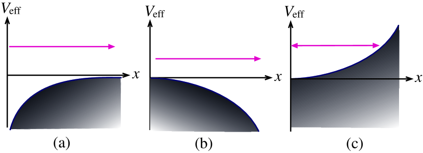
Figure 2: Effective potentials for the short wavelength perturbations. (a) is for $-1<w<1/3$, (b) is for $1/3<w<5/9$ and (c) is for $5/9<w<1$. For $-1<w<1/3,5/9<w<1$, inhomogeneity reduces the expansion rate of the Universe. For $1/3<w<5/9$, inhomogeneity enhances the expansion of the Universe. For $w=1/3,5/9$, there is no back reaction effect.

The back reaction effect of the short wavelength perturbation on the expansion of the Universe is summarized as follows (FIG. 2):

• $-1<w<1/3$ : The inhomogeneity reduces the expansion rate.

• $w=1/3$ : $V_{\text{eff}}=0$. The equation of state of the back reaction term is the same as the back ground matter field and we have no back reaction from inhomogeneity.

• $1/3<w<5/9$ : The inhomogeneity increases the expansion rate.

• $w=5/9$ : $V_{\text{eff}}=0$. There is no back reaction.

• $5/9<w<1$ : The inhomogeneity reduces the expansion rate and the Universe will recollapse.

V summary and discussion

In this paper, we applied the renormalization group method to the perturbed Einstein’s equation and derived the evolution equation for the renormalized scale factor. The renormalized scale factor includes the back reaction effect caused by the inhomogeneity of the first order perturbation. The resulting equation has the same form as the standard FRW equation with the back reaction effect appears as the effective energy density and pressure on the right hand side of the equation. For the long wavelength perturbation, the equation of the state of the back reaction terms depends on the value $w$. We have $p_{\text{BR}}=-\rho_{\text{BR}}/3,\rho_{\text{BR}}>0$ for $w=-1$ and this is equivalent to a negative spatial curvature. For $w=0$, we have $p_{\text{BR}}=-\rho_{\text{BR}}/3,\rho_{\text{BR}}<0$ and this is equivalent to a positive spatial curvature. On the other hand, for the short wavelength perturbation, the equation of state of the back reaction term becomes independent of $w$ and $p_{\text{BR}}\approx\rho_{\text{BR}}/3$. For $w<5/9$, $\rho_{\text{BR}}>0$ and the equation of state is the same as a radiation fluid.

We derived the effective FRW equation (34a) and (34b) without using the explicit form of the background solution and the perturbation solution. Usually, the renormalization group method is utilized to obtain the globally valid approximated solution of the differential equation and we must prepare naive perturbative solution of the original equation before applying the procedure of renormalization. In this paper, we could obtain the evolution equation for the renormalized scale factor without solving the perturbation equations. Once the effective FRW equation is obtained, it is possible to investigate the evolution of the effective scale factor and the back reaction effect by numerical method. Hence this approach is useful for the cosmological model with the scalar field in which case obtaining the solution of the perturbation is not easy in general.

ACKNOWLEDGMENT

This work was supported in part by a Grant-In-Aid for Scientific Research of the Ministry of Education, Science, Sports, and Culture of Japan (11640270).

References

• Issacson (1968) R. A. Issacson, Phys. Rev. 166, 1263 (1968).
• Futamase (1989) T. Futamase, Mon. Not. R. astr. Soc. 237, 187 (1989).
• Futamase (1996) T. Futamase, Phys. Rev. D 53, 681 (1996).
• Russ et al. (1997) H. Russ, M. H. Soffel, M. Kasai, and G. Börner, Phys. Rev. D 56, 2044 (1997).
• Boersma (1998) J. P. Boersma, Phys. Rev. D 57, 798 (1998).
• Mukhanov et al. (1997) V. M. Mukhanov, L. R. Abramo, and R. H. Brandenberger, Phys. Rev. Lett. 78, 1624 (1997).
• Abramo et al. (1997) L. R. Abramo, R. H. Brandenberger, and V. M. Mukhanov, Phys. Rev. D 56, 3248 (1997).
• Abramo (1997) L. R. Abramo, Ph.D. thesis, Brown University (1997), bROWN-HET-1096, gr-qc/9709049.
• Abramo (1999) L. R. Abramo, Phys. Rev. D D60, 064004 (1999).
• Nambu (2000) Y. Nambu, Phys. Rev. D 62, 104010 (2000), gr-qc/0006031.
• Nambu (2001) Y. Nambu, Phys. Rev. D 63, 044013 (2001).
• Chen et al. (1996) L.-Y. Chen, N. Goldenfeld, and Y. Oono, Phys. Rev. E 54, 376 (1996).
• Kunihiro (1995) T. Kunihiro, Prog. Theor. Phys. 94, 503 (1995).
• Goto et al. (1999) S. Goto, Y. Masutomi, and K. Nozaki, Prog. Theor. Phys. 102, 471 (1999).
• Nambu and Yamaguchi (1999) Y. Nambu and Y. Yamaguchi, Phys. Rev. D 60, 104011 (1999).
• Kodama and Sasaki (1984) H. Kodama and M. Sasaki, Prog. Theor. Phys. Suppliment 78, 1 (1984).
• Mukhanov et al. (1992) V. F. Mukhanov, H. A. Feldman, and R. H. Brandenberger, Phys. Rep. 215, 203 (1992).
• Hwang (1991) J. Hwang, ApJ 375, 443 (1991).