Asymptotically flat and regular Cauchy data

Abstract

I describe the construction of a large class of asymptotically flat initial data with non-vanishing mass and angular momentum for which the metric and the extrinsic curvature have asymptotic expansions at space-like infinity in terms of powers of a radial coordinate. I emphasize the motivations and the main ideas behind the proofs.

1 Introduction

Suppose we want to describe an isolated self-gravitating system. For example a star, a binary system, a black hole or colliding black holes. Typically these astrophysical systems are located far away from the Earth, so that we can receive from them only electromagnetic and gravitational radiation. How is this radiation? For example one can ask how much energy is radiated, or which are the typical frequencies for some systems. This is the general problem we want to study. These systems are expected to be described by the Einstein field equations. It is in principle possible to measure this radiation and compare the results with the predictions of the equations.

There are no explicit solution to the Einstein equations that can describe such systems. Since the equations are very complicated it is hard to believe that such explicit solution can ever be founded. Instead of trying to solve the complete equations at once, we use the so called 3+1 decomposition. We split the equations into “constraint” and “evolution”. First we give appropriate initial data: that is, a solution of the constraint equations. Once we have chosen the initial data, the problem is completely fixed. Then, we use the evolution equations to calculate the whole space-time. From the evolution we can compute physical relevant quantities like the wave form of the emitted gravitational wave. This method of solving the equations is consistent with the idea that in physic we want to make predictions, that is: knowing the system at a given time we want to predict its behavior in the future. It is of course in general very hard to compute the evolution of the data, one has to use numerical techniques. The question we want to study here is: what are the appropriate initial data for an isolated system?

We can think of initial data for Einstein’s equation as given a picture of the space time at a given time. It consists of a three dimensional manifold $\tilde{S}$ with some fields on it. The fields must satisfy the constraint equations. If the data describe an isolated system, the manifold $\tilde{S}$ is naturally divided in two regions. One compact region $\Omega$ which “contains the sources”, and its complement $\tilde{S}\setminus\Omega$ which is unbounded. We will call the latter one the asymptotic region. Of course, $\Omega$ can be as large as we want, the only requirement is that it be bounded. The fact that $\tilde{S}\setminus\Omega$ is unbounded means that we can go as far a we want from the source region $\Omega$, this capture the idea that the sources in $\Omega$ are isolated. That “the sources are in $\Omega$” suggest that the field decays in $\tilde{S}\setminus\Omega$. Then, the initial data approach flat initial data near infinity. We call them asymptotically flat initial data. An opposite situation is when we want to study the universe as a whole. In this case one usually consider initial data where the manifold $\tilde{S}$ is compact without boundary.

Figure 1: Initial data for two stars. The region $\Omega$ contains the matter sources, which are represented by black regions. The manifold $\tilde{S}$ is $\mathbb{R}^{3}$.

The simplest and most important example of asymptotically flat initial data is the case when $\tilde{S}$ is $\mathbb{R}^{3}$ and $\Omega$ some ball. Such data can describe, for example, ordinary stars. Consider an initial data set for a binary system, as is shown in Fig. 1. The stars are inside $\Omega$. Ordinary stars emit light, then in the asymptotic region we will have electromagnetic field beside the gravitational one. We can also have some dilute gas in this region. It is important to recall that we do not require vacuum in the asymptotic region. We only require that the field decays properly outside $\Omega$. However, in many situations it is a good approximation to assume vacuum in that region. When they evolve, the stars will follow some trajectory. Presumably an spiral orbit. The radius of the orbit will decrease with time, since the system loses energy in the form of gravitational waves. At late times, the system will settle down to a final stationary regime. This final state can be a rotating, stationary star. Or, if the initial data have enough mass concentrated in a small $\Omega$, a spinning black hole. We show the conformal diagrams of this two cases in Fig. 3 and Fig. 3. The gravitational radiation is measured at null infinity, where the observer is placed.

Figure 2: Conformal diagram of the space time generated by the initial data given in Fig. 1, in the case in which the final state is a stationary star.

Figure 3: Conformal diagram of the space time generated by the initial data given in Fig. 1, in the case in which the final state is a black hole.

Since the sources are in $\Omega$, the fields in this region can be very complicated. They depend on the kind of matter that forms the stars. Remarkable, even the topology of $\Omega$ can be complicated. The example in Fig. 1 has trivial topology, however non trivial topologies are relevant for black hole initial data. Consider the initial data for the Schwarzschild and Kerr black hole. In this case $\tilde{S}=S^{2}\times\mathbb{R}$ and $\Omega=S^{2}\times[-a,a]$ for some constant $a$, as it is shown in Fig. 5. The asymptotic region of these data has two disconnected components $\tilde{S}\setminus\Omega=\tilde{S}_{1}+\tilde{S}_{2}$. Each component is diffeomorphic to $\mathbb{R}^{3}$ minus a compact ball. We say that the data have two asymptotic ends. That is, there exist two disconnected “infinities”. Observations can be made in one of them but not in both. It is not clear the physical relevance of this extra asymptotic end. A normal collapse, as is shown in Fig. 3, will not have it. Therefore, one can think that only one asymptotic end is astrophysically relevant, being the other one just a mathematical peculiarity. The topology is not fixed by the Einstein equations. In this sense it remains quite arbitrary, one can thing that it is a kind of boundary conditions that has to be extra imposed to the equations. However, non trivial topologies appear naturally in the study of vacuum stationary black holes. A space time is stationary if it admits a timelike Killing vector field. The Schwarzschild and Kerr metrics are stationary. One can prove that every vacuum stationary asymptotically flat space time with trivial topology must be Minkowski. That is the non trivial topology is the “source” of the gravitational field in the vacuum stationary space times. In Fig. 5 we show another example with different a topology, in this case we have only one asymptotic end. Other topologies with many asymptotic ends are of interest because their evolution in time may describe the collision of several black holes. In Fig. 10 and Fig. 12 we show some examples.

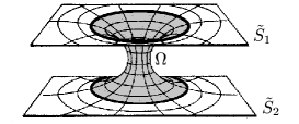
Figure 4: One black hole initial data. The asymptotic region has two disjoint components $\tilde{S}_{1}$ and $\tilde{S}_{2}$. The compact set $\Omega$ is represented by the shadowed region.

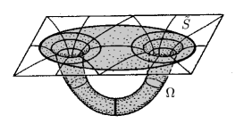
Figure 5: Initial data for a Misner wormhole Misner60 . The asymptotic region has only one component. The compact set $\Omega$ is represented by the shadowed region.

One usually has the idea that the matter sources generate gravitational field. To some extend this is true for many cases of astrophysical interest. However, as we have seen, a pure vacuum initial data with non trivial topologies can have mass. Moreover, one can also have a pure gravitational radiation initial data, that is a vacuum initial data with trivial topology with non zero mass. These kind of data are important in order to understand properties of the radiation itself which do not depend on the specific matter models. It is even possible to form a black hole with these type of data (see Beig91c ).

In contrast to $\Omega$, the asymptotic region is very simple. The fields on it are approximately flat and its topology is $\mathbb{R}^{3}$ minus a compact ball. We want to analyze the fields in this region. It is of course true that the fields there are determined by the fields in $\Omega$. But some important properties of them do not depend very much on the detailed structure of the sources in $\Omega$. The most important of these properties is that the initial data will have a positive mass if the sources satisfies some energy condition. In this article we want to study some other properties of the fall of the fields in the asymptotic region which will be also independent on the sources in $\Omega$. It is important to note that we can only measure precisely this kind of properties, because we can not prepare the initial conditions of an astrophysical system in the laboratory and then it is impossible to find the exact initial data for a real system. We can only analyze those effects which do not depend very much on fine details of the sources.

In order to simplify the hypothesis of the theorems, we will assume in this article that there are no matter sources in $\tilde{S}$. All the results will remain valid under suitable assumptions on the matters sources.

We summarize the discussion above in the following definition. An initial data set for the Einstein vacuum equations is given by a triple $(\tilde{S},\tilde{h}_{ab},\tilde{\Psi}_{ab})$ where $\tilde{S}$ is a connected 3-dimensional manifold, $\tilde{h}_{ab}$ a (positive definite) Riemannian metric, and $\tilde{\Psi}_{ab}$ a symmetric tensor field on $\tilde{S}$. They satisfy the vacuum constraint equations

$$\tilde{D}^{b}\tilde{\Psi}_{ab}-\tilde{D}_{a}\tilde{\Psi}=0,$$ (1)

$$\tilde{R}+\tilde{\Psi}^{2}-\tilde{\Psi}_{ab}\tilde{\Psi}^{ab}=0,$$ (2)

on $\tilde{S}$, where $\tilde{D}_{a}$ is the covariant derivative with respect to $\tilde{h}_{ab}$, $\tilde{R}$ is the trace of the corresponding Ricci tensor, and $\tilde{\Psi}=\tilde{h}^{ab}\tilde{\Psi}_{ab}$. The data will be called asymptotically flat with $N$ asymptotic ends, if for some compact set $\Omega$ we have that $\tilde{S}\setminus\Omega=\sum_{k=1}^{N}\tilde{S}_{k}$, where $\tilde{S}_{k}$ are open sets such that each $\tilde{S}_{k}$ can be mapped by a coordinate system $\tilde{x}^{j}$ diffeomorphically onto the complement of a closed ball in $\mathbb{R}^{3}$ such that we have in these coordinates

$$\tilde{h}_{ij}=(1+\frac{2m}{\tilde{r}})\delta_{ij}+O(\tilde{r}^{-2}),$$ (3)

$$\tilde{\Psi}_{ij}=O(\tilde{r}^{-2}),$$ (4)

as $\tilde{r}=(\sum_{j=1}^{3}({\tilde{x}^{j}})^{2})^{1/2}\to\infty$ in each set $\tilde{S}_{k}$. Here the constant $m$ denotes the mass of the data, $a,b,c...$ denote abstract indices, $i,j,k...$, which take values $1,2,3$, denote coordinates indices while $\delta_{ij}$ denotes the flat metric with respect to the given coordinate system $\tilde{x}^{j}$. Tensor indices will be moved with the metric $h_{ab}$ and its inverse $h^{ab}$. We set $x_{i}=x^{i}$ and $\partial^{i}=\partial_{i}$. These conditions guarantee that the mass, the momentum, and the angular momentum of the initial data set are well defined in every end.

We want to analyze the higher order terms in (3) and (4). For example, the terms $O(\tilde{r}^{-2})$ could have the form $\tilde{r}^{-2}\sin(\tilde{r}^{10})$. This function is certainly $O(\tilde{r}^{-2})$, but any derivative of it will blow up at infinity. Should such complicated terms be admissible in a description of a realistic isolated systems? In Newton’s theory and Electromagnetism one can give a definitive answer to this question: the fields have a fall off behavior like powers in a radial coordinate. Take for example a matter density $\rho$ with compact support. The Newton’s gravitational potential $u$ satisfies the Poisson equation

$$\Delta u=4\pi\rho,$$ (5)

where $\Delta$ is the Laplacian. Outside the support of $\rho$ the potential $u$ satisfies $\Delta u=0$. It is a well known that every harmonic function that goes to zero at infinity has an expansion of the form

$$u=\sum_{k\geq 1}\frac{u^{k-1}}{\tilde{r}^{k}},$$ (6)

where $u^{k}$ are the spherical harmonics of order $k$. In this case the field equations force the potential to have the fall off behavior (6).

The situation for the Einstein equation is more complicate. In analogy with (6), one can ask the question whether there exist a class of initial data such that the metric and the extrinsic curvature admit near space-like infinity asymptotic expansions of the form

$$\tilde{h}_{ij}\sim(1+\frac{2m}{\tilde{r}})\delta_{ij}+\sum_{k\geq 2}\frac{\tilde{h}^{k}_{ij}}{\tilde{r}^{k}},$$ (7)

$$\tilde{\Psi}_{ij}\sim\sum_{k\geq 2}\frac{\tilde{\Psi}^{k}_{ij}}{\tilde{r}^{k}},$$ (8)

where $\tilde{h}^{k}_{ij}$ and $\tilde{\Psi}^{k}_{ij}$ are smooth function on the unit 2-sphere (thought as being pulled back to the spheres $\tilde{r}=const.$ under the map $\tilde{x}^{j}\rightarrow\tilde{x}^{j}/\tilde{r}$). In this article I want to give an answer to this question. It is not only for convenience or aesthetic reasons that we want to avoid terms like $\tilde{r}^{-2}\sin(\tilde{r}^{10})$ in the expansions. They are also very difficult to handle numerically.

In order to see how the gravitational field behaves near infinity, it is natural to study first some examples. Consider asymptotically flat static space-times. We say that a space-time is static if it admits a hypersurface orthogonal time like Killing vector. One can take one of this hypersurfaces and analyze the fields $\tilde{h}_{ab}$ and $\tilde{\Psi}_{ab}$ on it. The simplest static space time is the Schwarzschild metric. In this case we have $\tilde{h}_{ij}=(1+m/(2\tilde{r}))^{4}\delta_{ij}$, $\tilde{\Psi}_{ij}=0$, which is certainly of the form (7), (8). For general static, asymptotically flat space times it can be proved that the initial data have also asymptotic expansions of the form (7) and (8). Moreover, in this case the fields are analytic functions of the coordinates. Then the expansions (7) and (8) are in fact convergent powers series, in analogy with (6). This result is far from being obvious. It was proved by Beig and Simon in Beig80 based on an early work by Geroch Geroch70 .

One can go a step further and consider asymptotically flat stationary solutions. A stationary space time admits a timelike Killing field which is in general non hypersurface orthogonal. These space times describe rotating stars in equilibrium. The twist of the Killing vector is related to the angular velocity of the star. In this case there are no preferred hypersurfaces. The most important example of stationary solution is the Kerr metric. It can be seen that for $t=const.$ slice of the Kerr metric in the standard Boyer-Lindquist coordinates the fields $\tilde{h}_{ab}$ and $\tilde{\Psi}_{ab}$ satisfy (7) and (8). For general stationary asymptotically flat solutions there also exist slices such that (7) and (8) holds. The essential part of this result was also proved by Beig and Simon in Beig81 (see also Kundu81 ). However, in these works the expansions are made in the abstract manifold of the orbits of the Killing vector field. In contrast with the static case this manifold does not correspond to any hypersurface of the space time. One has to translate this result in terms of the metric and the extrinsic curvature of some slices. This last step was made in Dain01b . As in the static case, the fields are analytic functions of the coordinates.

We have shown that there exist non trivial examples of initial data which satisfies (7) and (8). But how general are these expansions? For example, is it possible to have data with gravitational radiation that satisfies (7) and (8)? I want to show that in fact there exists a large class of asymptotically flat initial data which have the asymptotic behavior (7) and (8). These data will not be, in general, stationary.

The interest in such data is twofold. First, the evolution of asymptotically flat initial data near space-like and null infinity has been studied in considerable detail in Friedrich98 . In that article has been derived in particular a certain “regularity condition” on the data near space-like infinity, which is expected to provide a criterion for the existence of a smooth asymptotic structure at null infinity. To simplify the lengthy calculations, the data considered in Friedrich98 have been assumed to be time-symmetric and to admit a smooth conformal compactification. With these assumptions the regularity condition is given by a surprisingly succinct expression. With the present work we want to provide data which will allow us to perform the analysis of Friedrich98 without the assumption of time symmetry but which are still “simple” enough to simplify the work of generalizing the regularity condition to the case of non-trivial second fundamental form. Second, the “regular finite initial value problem near space-like infinity”, formulated and analyzed in Friedrich98 , suggests how to calculate numerically entire asymptotically flat solutions to Einstein’s vacuum field equations on finite grids. In the present article I provide data for such numerical calculations which should allow us to study interesting situations while keeping a certain simplicity in the handling of the initial data.

The difficulty of constructing data with the asymptotic behavior (7), (8) arises from the fact that the fields need to satisfy the constraint equations (1) and (2). Part of the data, the “free data”, can be given such that they are compatible with (7), (8). However, the remaining data are governed by elliptic equations (the constraint equations will reduce to elliptic equations as we will see below) and we have to show that (7), (8) are in fact a consequence of the equations and the way the free data have been prescribed.

To employ the standard techniques to provide solutions to the constraints, we assume

$$\tilde{\Psi}=0,$$ (9)

such that the data correspond to a hypersurface which is maximal in the solution space-time.

I give an outline of the results which are available so far (see Dain99 and Dain01 for more details and proofs). Because of the applications indicated above, we wish to control in detail the conformal structure of the data near space-like infinity. Therefore we shall analyze the data in terms of the conformal compactification $(S,h_{ab},\Psi_{ab})$ of the “physical” asymptotically flat data. Here $S$ denotes a smooth, connected, orientable, compact 3-manifold. Take an arbitrary point $i$ in $S$ and define $\tilde{S}=S\backslash\{i\}$. The point $i$ will represent, in a sense described in detail below, space-like infinity for the physical initial data. The physical manifold $\tilde{S}$ is essentially the stereographic projection of the compact manifold $S$. For example if we chose $S$ to be $S^{3}$ then $\tilde{S}$ will be $\mathbb{R}^{3}$.

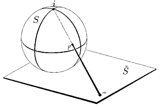
Figure 6: The stereographic projection of $S^{3}$ in $\mathbb{R}^{3}$. A neighborhood $B_{a}$ of the point $i$ is mapped into the asymptotic region of the physical manifold $\tilde{S}$.

Working with $S$ and not with $\tilde{S}$, has several technical advantage. It is simpler to prove existence of solutions for an elliptic equation on a compact manifold than in a non compact one. The price that we have to pay is that the equations will be singular at $i$. However this singularity is mild. It is also simpler to analyze the fields in terms of local differentiability in a neighborhood of $i$ than in terms of fall off expansions at infinity in $\tilde{S}$. Moreover, this technique is also useful to construct initial data with non-trivial topology. By singling out more points in $S$ and by treating the fields near these points in the same way as near $i$ we could construct data with several asymptotically flat ends. In Fig. 8 – 14 we show some examples. All the following arguments equally apply to such situations, however, for convenience we restrict ourselves to the case of a single asymptotically flat end.

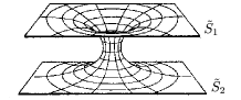
Figure 7: Initial data with two asymptotic ends.

Figure 8: A compactification of these data in the sphere.

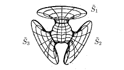
Figure 9: The Brill-Lindquist initial data for two black holes Brill63 . The data have three asymptotic ends.

Figure 10: A compactification of these data in the sphere.

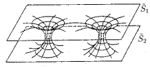
Figure 11: The Misner initial data for two black holes Misner63 . The data have three asymptotic ends.

Figure 12: A compactification of these data in the torus.

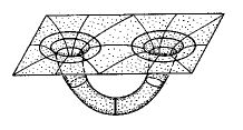
Figure 13: The Misner wormhole initial data. The data have only one asymptotic end.

Figure 14: A compactification of these data in the torus.

We assume that $h_{ab}$ is a positive definite metric on $S$ with covariant derivative $D_{a}$ and $\Psi_{ab}$ is a symmetric tensor field which is smooth on $\tilde{S}$. In agreement with (9) we shall assume that $\Psi_{ab}$ is trace free,

$$h^{ab}\,\Psi_{ab}=0.$$

The fields above are related to the physical fields by rescaling

$$\tilde{h}_{ab}=\theta^{4}\,h_{ab},\,\,\,\,\,\,\,\tilde{\Psi}_{ab}=\theta^{-2}\,\Psi_{ab},$$ (10)

with a conformal factor $\theta$ which is positive on $\tilde{S}$. For the physical fields to satisfy the vacuum constraints we need to assume that

$$D^{a}\Psi_{ab}=0\quad\mbox{on}\quad\tilde{S},$$ (11)

$$(D_{b}D^{b}-\frac{1}{8}R)\theta=-\frac{1}{8}\Psi_{ab}\Psi^{ab}\theta^{-7}\quad\mbox{on}\quad\tilde{S}.$$ (12)

Equation (12) for the conformal factor $\theta$ is the Lichnerowicz equation, transferred to our context.

Let $x^{j}$ be $h$-normal coordinates centered at $i$ such that $h_{kl}=\delta_{kl}$ at $i$ and set $r=(\sum_{i=1}^{3}(x^{j})^{2})^{1/2}$. To ensure asymptotical flatness of the data (10) we require

$$\Psi_{ab}=O(r^{-4})\quad\mbox{as}\quad r\rightarrow 0,$$ (13)

$$\lim_{r\to 0}r\theta=1.$$ (14)

In the coordinates $\tilde{x}^{j}=x^{j}/r^{2}$ the fields (10) will then satisfy (3), (4) (cf. Friedrich88 , Friedrich98 for this procedure).

Not all data as given by (10), which are derived from data $h_{ab}$, $\Psi_{ab}$ as described above, will satisfy conditions (7), (8). We will have to impose extra conditions and we want to keep these conditions as simple as possible.

Since we assume the metric $h_{ab}$ to be smooth on $S$, it will only depend on the behavior of $\theta$ near $i$ whether condition (7) will be satisfied. Via equation (12) this behavior depends on $\Psi_{ab}$. What kind of condition do we have to impose on $\Psi_{ab}$ in order to achieve (7) ?

The following space of functions will play an important role in our discussion. Denote by $B_{a}$ the open ball with center $i$ and radius $r=a>0$, where $a$ is chosen small enough such that $B_{a}$ is a convex normal neighborhood of $i$. A function $f\in C^{\infty}(\tilde{S})$ is said to be in $E^{\infty}(B_{a})$ if on $B_{a}$ we can write $f=f_{1}+rf_{2}$ with $f_{1},f_{2}\in C^{\infty}(B_{a})$ (cf. definition 1). An answer to our question is given by following theorem:

Theorem 1.1

Let $h_{ab}$ be a smooth metric on $S$ with positive Ricci scalar $R$. Assume that $\Psi_{ab}$ is smooth in $\tilde{S}$ and satisfies on $B_{a}$

$$r^{8}\Psi_{ab}\Psi^{ab}\in E^{\infty}(B_{a}).$$ (15)

Then there exists on $\tilde{S}$ a unique solution $\theta$ of equation (12), which is positive, satisfies (14), and has in $B_{a}$ the form

$$\theta=\frac{\hat{\theta}}{r},\quad\hat{\theta}\in E^{\infty}(B_{a}),\quad\hat{\theta}(i)=1.$$ (16)

In fact, we will get slightly more detailed information. We find that $\hat{\theta}=u_{1}+r\,u_{2}$ on $B_{a}$ with $u_{2}\in E^{\infty}(B_{a})$ and a function $u_{1}\in C^{\infty}(B_{a})$ which satisfies $u_{1}=1+O(r^{2})$ and

$$(D_{b}D^{b}-\frac{1}{8}R)\frac{u_{1}}{r}=\theta_{R},$$

in $B_{a}\backslash\{i\}$, where $\theta_{R}$ is in $C^{\infty}(B_{a})$ and vanishes at any order at $i$.

If $\theta$ has the form (16) then (7) will be satisfied due to our assumptions on $h_{ab}$.

Note the simplicity of condition (15). If the metric is analytic on $B_{a}$ it can be arranged that $\theta_{R}=0$ and $u_{1}$ is analytic on $B_{a}$ (and unique with this property, see Garabedian ). The requirement $R>0$, which ensures the solvability of the Lichnerowicz equation, could be reformulated in terms of a condition on the Yamabe number (cf. Lee87 ).

Theorem 1.1 has two parts. One is the existence and uniqueness of the solution. This part depends on global properties of the fields on $S$. It can be proved under much weaker assumptions on the differentiability of $h_{ab}$ and $\Psi_{ab}$. The second part concerns the regularly in $B_{a}$, and depends only on local properties of the fields in $B_{a}$. This part can also be proved under weaker hypothesis. These generalizations have physical relevance, I will come back to this point in the final section.

It remains to be shown that condition (15) can be satisfied by tensor fields $\Psi_{ab}$ which satisfy (11), (13). A special class of such solutions, namely those which extend smoothly to all of $S$, can easily be obtained by known techniques (cf. Choquet80 ). However, in that case the initial data will have vanishing momentum and angular momentum. To obtain data without this restriction, we have to consider fields $\Psi_{ab}\in C^{\infty}(\tilde{S})$ which are singular at $i$ in the sense that they admit, in accordance with (4), (10), (14), at $i=\{r=0\}$ asymptotic expansions of the form

$$\Psi_{ij}\sim\sum_{k\geq-4}\Psi^{k}_{ij}r^{k}\quad\mbox{with}\quad\Psi^{k}_{ij}\in C^{\infty}(S^{2}).$$ (17)

It turns out that condition (15) excludes data with non-vanishing linear momentum, which requires a non-vanishing leading order term of the form $O(r^{-4})$. In section 2 we will show that such terms imply terms of the form $\log\,r$ in $\theta$ and thus do not admit expansion of the form (7). However, this does not necessarily indicate that condition (15) is overly restrictive. In the case where the metric $h_{ab}$ is smooth it will be shown in section 2 that a non-vanishing linear momentum always comes with logarithmic terms, irrespective of whether condition (15) is imposed or not.

There remains the question whether there exist fields $\Psi_{ab}$ which satisfy (15) and have non-trivial angular momentum. The latter requires a term of the form $O(r^{-3})$ in (17). It turns out that condition (15) fixes this term to be of the form

$$\Psi_{AJ}^{ab}=\frac{A}{r^{3}}\,(3n^{a}n^{b}-\delta^{ab})+\frac{3}{r^{3}}(n^{a}\epsilon^{bcd}J_{c}n_{d}+n^{b}\epsilon^{acd}J_{c}n_{d}),$$ (18)

where $n^{i}=x^{i}/r$ is the radial unit normal vector field near $i$ and $J^{k}$, $A$ are constants, the three constants $J^{k}$ specifying the angular momentum of the data. The spherically symmetric tensor which appears here with the factor $A$ agrees with the extrinsic curvature for a maximal (non-time symmetric) slice in the Schwarzschild solution (see for example Beig98 ). Note that the tensor $\Psi_{AJ}^{ab}$ satisfies condition (15) and the equation $\partial_{a}\Psi^{ab}_{AJ}=0$ on $\tilde{S}$ for the flat metric, hence it is a non-trivial example. We want to study more general situations.

In the existence proof for equations (11) and (13), the possible existence of conformal Killing vectors $\xi^{a}$ of the metric $h_{ab}$ will play an important role. A conformal Killing vector is a solution on $S$ of $\mathcal{L}_{h}\xi=0$, where we have defined the conformal Killing operator

$$(\mathcal{L}_{h}v)^{ab}\equiv D^{a}v^{b}+D^{b}v^{a}-\frac{2}{3}\,h^{ab}\,D_{c}v^{c}.$$ (19)

Given $\xi^{a}$ we define the followings constants

$$S^{a}={\epsilon^{a}}_{bc}D^{b}\xi^{c}(i),\quad a=\frac{1}{3}D_{a}\xi^{a}(i).$$ (20)

The free-data in the solution $\Psi^{ab}$ consist in two pieces: a singular and a regular one, which we will denote by $\Phi^{ab}_{sing}$ and $\Phi^{ab}_{reg}$ respectively. We define $\Phi^{ab}_{sing}$ in $B_{a}\setminus\{i\}$ by

$$\Phi^{ab}_{sing}=\chi\,(\Psi_{AJ}^{ab}-\frac{1}{3}\,h_{cd}\,\Psi_{AJ}^{cd}\,{h}^{ab}),$$ (21)

and vanishes elsewhere. Here $\chi$ denotes a smooth function of compact support in $B_{a}$ equal to $1$ on $B_{a/2}$. We assume that $\Phi^{ab}_{reg}$ can be written near $i$ in the form

$$\Phi^{ab}_{reg}=r^{-3}\,\Phi^{ab}_{1reg}+\Phi^{ab}_{2reg},$$ (22)

where $\Phi^{ab}_{1reg}$, $\Phi^{ab}_{2reg}$ are smooth symmetric trace free tensors in $S$ and such that $\Phi^{ij}_{1reg}=O(r^{2})$, and $x_{i}\,x_{j}\,\Phi^{ij}_{1reg}=r^{2}\,\Phi$ with some $\Phi\in C^{\infty}(B_{a})$.

Theorem 1.2

Let $h_{ab}$ a smooth metric in $S$. Let $\Phi^{ab}_{sing}$ and $\Phi^{ab}_{reg}$ given by (21) and (22).

i) If the metric $h$ admits no conformal Killing fields on $S$, then there exists a unique vector field $v^{a}$ such that the tensor field

$$\Psi^{ab}=\Phi_{sing}^{ab}+\Phi_{reg}^{ab}+(\mathcal{L}_{h}v)^{ab},$$ (23)

satisfies the equation $D_{a}\Psi^{ab}=0$ in $S\setminus\{i\}$. The solution satisfies $\Psi_{ab}=O(r^{-3})$ at $i$ and condition (15).

ii) If the metric $h$ admits conformal Killing fields $\xi^{a}$ on $S$, a vector field $v^{a}$ as specified above exists if and only if the constants $J^{a}$, $A$ (partly) characterizing the tensor field $\Phi_{sing}^{ab}$ satisfy the equation

$$J^{a}\,S_{a}+A\,a=0,$$ (24)

for any conformal Killing field $\xi^{a}$ of $h$, where the constants $S_{a}$ and $a$ are given by (20).

In both cases the angular momentum of $\Psi^{ab}$ is given by $J^{a}$. This quantity can thus be prescribed freely in case (i).

Theorem 1.2, as Theorem 1.1, contains two parts. One is the existence and uniqueness of the solution $v^{a}$. The restriction (24) appears in this part. See Beig96 , Dain99 and Dain01d for a generalization and interpretation of this condition. The other part concerns the regularity of the solution in $B_{a}$, namely that it satisfies condition (15). This part depends only on local assumptions of the fields in $B_{a}$. We prove a more detailed version of this theorem in Dain99 .

2 Solution of the Hamiltonian Constraint with Logarithmic terms

Assume, for simplicity, that the metric $h_{ab}$ is conformally flat in $B_{a}$. Then the operator that appears in the left hand side of equation (12) reduce to the Laplacian $\Delta$. This simplification is of course a restriction on the allowed initial data, but it already contains all the main problems and the essential features of the more general case. It is also important to remark that even under this assumption it is possible to describe a rich family of initial data, since we are making restrictions only on $B_{a}$. Consider the Poisson equation (5). The example

$$\Delta(\log rh_{m})=r^{-2}h_{m}(2m+1),$$ (25)

where $h_{m}$ is an harmonic polynomial of order $m$ (i.e. $\Delta h_{m}=0$) shows that logarithmic terms can occur in solutions to the Poisson equation even if the source has only terms of the form $r^{s}p$ where $p$ is some polynomial. That is, even if our free data have expansion in powers of $r$ logarithmic terms will appear in the conformal factor $\theta$. We shall use this to show that logarithmic terms can occur in the solution to the Lichnerowicz equation if the condition $r^{8}\Psi_{ab}\Psi^{ab}\in E^{\infty}(B_{a})$ is not satisfied. Our example will be concerned with initial data with non-vanishing linear momentum.

We assume that in a small ball $B_{a}$ centered at $i$ the tensor $\Psi^{ab}$ has the form

$$\Psi^{ab}=\Psi_{P}^{ab}+\Psi_{R}^{ab},$$ (26)

where $\Psi_{P}^{ab}$ is given in normal coordinates by

$$\Psi_{P}^{ab}=\frac{3}{2r^{4}}\left(-P^{a}n^{b}-P^{b}n^{a}-(\delta^{ab}-5n^{a}n^{b})\,P^{c}n_{c}\right),$$ (27)

and $\Psi_{R}^{ab}=O(r^{-3})$ is a tensor field such that $\Psi^{ab}$ satisfies equation (11). We will assume also that $\Psi_{R}^{ab}$ satisfies some mild smoothness condition (cf. Dain99 ).

Since $\Psi_{P}^{ab}$ is trace-free and divergence-free with respect to the flat metric, we could, of course, choose $h_{ab}$ to be the flat metric and $\Psi_{R}^{ab}=0$. This would provide one of the conformally flat initial data sets discussed in York . We are interested in a more general situation.

Lemma 1

Let $h_{ab}$ be a smooth metric, and let $\Psi^{ab}$ be given by (26). Then, there exists a unique, positive, solution to the Hamiltonian constraint (12). In $B_{a}$ it has the form

$$\theta=\frac{w_{1}}{r}+\frac{1}{2}m+\frac{1}{32}\,r\,\left((9\,(P^{i}n_{i})^{2}-33\,P^{2}\right)\\ +\frac{7}{16}\,m\,r^{2}\,\left(\frac{5}{4}\,P^{2}+\frac{3}{5}\,(3\,(P^{i}n_{i})^{2}-P^{2})\,\log r\right)+u_{R},$$ (28)

where $P^{i}P_{i}=P^{2}$, the constant $m$ is the total mass of the initial data, $w_{1}$ is a smooth function with $w_{1}=1+O(r^{2})$, and $u_{R}\in C^{2,\alpha}(B_{a})$ with $u_{R}(0)=0$.

Since $w_{1}$ is smooth and $u_{R}$ is in $C^{2,\alpha}(B_{a})$, there cannot occur a cancellation of logarithmic terms. For non-trivial data, for which $m\neq 0$, the logarithmic term will always appear. In the case where $h_{ab}$ is flat (in this case we have $w_{1}=1$) and $\Psi_{R}^{ab}=0$ an expansion similar to (28) has been calculated in Gleiser99 .

3 Explicit solutions of the momentum constraint

Instead of given the proof of Theorem 1.2, in this section I want to present some explicit solutions of equation (11) for conformally flat and also for axially symmetric metrics. In the first case we will construct all the solutions, in the second one only some of them. We will show how to achieve condition (15) in terms of the free data. In both cases the solution is constructed in terms of derivatives of some free functions. That makes them suitable for explicit computations. In particular, if we assume that these free functions have compact support, then $\Psi^{ab}$ will also have compact support. We note incidentally that, as an application, one can easily construct regular hyperboloidal initial data with non-trivial extrinsic curvature.

3.1 The momentum constraint on Euclidean space

In the following we shall give an explicit constructing of the smooth solutions to the equation $\partial_{a}\Psi^{ab}=0$ on the 3-dimensional Euclidean space $\mathbb{E}^{3}$ (in suitable coordinates $\mathbb{R}^{3}$ endowed with the flat standard metric) or open subsets of it. Another method to obtain such solutions has been described in Beig96' , multipole expansions of such tensors have been studied in Beig96 .

Let $i$ be a point of $\mathbb{E}^{3}$ and $x^{k}$ a Cartesian coordinate system with origin $i$ such that in these coordinates the metric of $\mathbb{E}^{3}$, denoted by $\delta_{ab}$, is given by the standard form $\delta_{kl}$. We denote by $n^{a}$ the vector field on $\mathbb{E}^{3}\setminus\{i\}$ which is given in these coordinates by $x^{k}/|x|$.

Denote by $m_{a}$ and its complex conjugate $\bar{m}_{a}$ complex vector fields, defined on $\mathbb{E}^{3}$ outside a lower dimensional subset and independent of $r=|x|$, such that

$$m_{a}m^{a}=\bar{m}_{a}\bar{m}^{a}=n_{a}m^{a}=n_{a}\bar{m}^{a}=0,\,\,\,\,\,\,m_{a}\bar{m}^{a}=1.$$ (29)

There remains the freedom to perform rotations $m_{a}\rightarrow e^{if}m_{a}$ with functions $f$ which are independent of $r$.

The metric has the expansion

$$\delta_{ab}=n_{a}n_{b}+\bar{m}_{a}m_{b}+m_{a}\bar{m}_{b},$$

while an arbitrary symmetric, trace-free tensor $\Psi_{ab}$ can be expended in the form

$$r^{3}\Psi_{ab}=\xi(3n_{a}n_{b}-\delta_{ab})+\sqrt{2}\eta_{1}n_{(a}\bar{m}_{b)}+\sqrt{2}\bar{\eta}_{1}n_{(a}m_{b)}+\\ \bar{\mu}_{2}m_{a}m_{b}+\mu_{2}\bar{m}_{a}\bar{m}_{b},$$ (30)

with

$$\xi=\frac{1}{2}r^{3}\Psi_{ab}n^{a}n^{b},\quad\eta_{1}=\sqrt{2}r^{3}\Psi_{ab}n^{a}m^{b},\quad\mu_{2}=r^{3}\Psi_{ab}m^{a}m^{b}.$$

Since $\Psi_{ab}$ is real, the function $\xi$ is real while $\eta_{1}$, $\mu_{2}$ are complex functions of spin weight 1 and 2 respectively.

Using in the equation

$$\partial_{a}\Psi^{ab}=0,$$ (31)

the expansion (30) and contracting suitably with $n^{a}$ and $m^{a}$, we obtain the following representation of (31)

$$4r\partial_{r}\xi+\bar{\eth}\eta_{1}+\eth\bar{\eta}_{1}=0,$$ (32)

$$r\partial_{r}\eta_{1}+\bar{\eth}\mu_{2}-\eth\xi=0.$$ (33)

Here $\partial_{r}$ denotes the radial derivative and $\eth$ the edth operator of the unit two-sphere (cf. Penrose for definition and properties). By our assumptions the differential operator $\eth$ commutes with $\partial_{r}$.

Let ${}_{s}Y_{lm}$ denote the spin weighted spherical harmonics, which coincide with the standard spherical harmonics $Y_{lm}$ for $s=0$. The ${}_{s}Y_{lm}$ are eigenfunctions of the operator $\bar{\eth}\eth$ for each spin weight $s$. More generally, we have

$$\bar{\eth}^{p}\eth^{p}({}_{s}Y_{lm})=(-1)^{p}\frac{(l-s)!}{(l-s-p)!}\frac{(l+s+p)!}{(l+s)!}{}_{s}Y_{lm}.$$ (34)

If $\mu_{s}$ denotes a smooth function on the two-sphere of integral spin weight $s$, there exists a function $\mu$ of spin weight zero such that $\eta_{s}=\eth^{s}\eta$. We set $\eta^{R}=\textnormal{Re}(\eta)$ and $\eta^{I}=i\,\textnormal{Im}(\eta)$, such that $\eta=\eta^{R}+\eta^{I}$, and define

$$\eta_{s}^{R}=\eth^{s}\eta^{R},\,\,\,\eta_{s}^{I}=\eth^{s}\eta^{I},$$

such that $\eta_{s}=\eta_{s}^{R}+\eta_{s}^{I}$. We have

$$\overline{\eth^{s}\eta^{R}}=\bar{\eth}^{s}\eta^{R},\,\,\,\overline{\eth^{s}\eta^{I}}=-\bar{\eth}^{s}\eta^{I}.$$

Using these decompositions now for $\eta_{1}$ and $\mu_{2}$, we obtain equation (32) in the form

$$2r\partial_{r}\xi=-\bar{\eth}\eth\eta^{R}.$$ (35)

Applying $\bar{\eth}$ to both sides of equation (33) and decomposing into real and imaginary part yields

$$r\partial_{r}\bar{\eth}\eth\eta^{I}=-\bar{\eth}^{2}\eth^{2}\mu^{I}$$ (36)

$$2r\partial_{r}(r\partial_{r}\xi)+\bar{\eth}\eth\xi=\bar{\eth}^{2}\eth^{2}\mu^{R}.$$ (37)

Since the right hand side of (35) has an expansion in spherical harmonics with $l\geq 1$ and the right hand sides of (36), (37) have expansions with $l\geq 2$, we can determine the expansion coefficients of the unknowns for $l=0,1$. They can be given in the form

$$\xi=A+rQ+\frac{1}{r}P,\quad\eta^{I}=iJ+const.,\quad\eta^{R}=rQ-\frac{1}{r}P+const.,$$

with

$$P=\frac{3}{2}P^{a}n_{a},\quad Q=\frac{3}{2}Q^{a}n_{a},\quad J=3J^{a}n_{a},$$ (38)

where $A,P^{a},Q^{a},J^{a}$ are arbitrary constants. Using (30), we obtain the corresponding tensors in the form (cf. (York )

$$\Psi_{P}^{ab} =\frac{3}{2r^{4}}\left(-P^{a}n^{b}-P^{b}n^{a}-(\delta^{ab}-5n^{a}n^{b})\,P^{c}n_{c}\right),$$ (39)

$$\Psi_{J}^{ab} =\frac{3}{r^{3}}(n^{a}\epsilon^{bcd}J_{c}n_{d}+n^{b}\epsilon^{acd}J_{c}n_{d}),$$ (40)

$$\Psi_{A}^{ab} =\frac{A}{r^{3}}\,(3n^{a}n^{b}-\delta^{ab}),$$ (41)

$$\Psi_{Q}^{ab} =\frac{3}{2r^{2}}\left(Q^{a}n^{b}+Q^{b}n^{a}-(\delta^{ab}-n^{a}n^{b})\,Q^{c}n_{c}\right).$$ (42)

We assume now that $\xi$ and $\eta^{I}$ have expansions in terms of in spherical harmonics with $l\geq 2$. Then there exists a smooth function $\lambda_{2}$ of spin weight 2 such that

$$\xi=\bar{\eth}^{2}\lambda_{2}^{R},\quad\eta_{1}^{I}=\bar{\eth}\lambda_{2}^{I}.$$

Using these expressions in equations (35) – (37) and observing that for smooth spin weighted functions $\mu_{s}$ with $s>0$ we can have $\bar{\eth}\mu_{s}=0$ only if $\mu_{s}=0$, we obtain

$$\eth\eta^{R}=-2r\partial_{r}\bar{\eth}\lambda_{2}^{R},\quad\eth^{2}\mu^{I}=-r\partial_{r}\lambda_{2}^{I},$$

$$\eth^{2}\mu^{R}=2r\partial_{r}(r\partial_{r}\lambda_{2}^{R})-2\lambda_{2}^{R}+\eth\bar{\eth}\lambda_{2}^{R}.$$

We are thus in a position to describe the general form of the coefficients in the expression (30)

$$\xi =\bar{\eth}^{2}\lambda_{2}^{R}+A+r\,Q+\frac{1}{r}\,P,$$ (43)

$$\eta_{1} =-2\,r\,\partial_{r}\,\bar{\eth}\lambda_{2}^{R}+\bar{\eth}\lambda_{2}^{I}+r\,\eth Q-\frac{1}{r}\,\eth P+i\,\eth J,$$ (44)

$$\mu_{2} =2\,r\,\partial_{r}(r\,\partial_{r}\,\lambda_{2}^{R})-2\,\lambda_{2}^{R}+\eth\bar{\eth}\lambda_{2}^{R}-r\,\partial_{r}\,\lambda_{2}^{I}.$$ (45)

Theorem 3.1

Let $\lambda$ be an arbitrary complex $C^{\infty}$ function in $B_{a}\setminus\{i\}\subset\mathbb{E}^{3}$ with $0<a\leq\infty$, and set $\lambda_{2}=\eth^{2}\lambda$. Then the tensor field

$$\Psi^{ab}=\Psi_{P}^{ab}+\Psi_{J}^{ab}+\Psi_{A}^{ab}+\Psi_{Q}^{ab}+\Psi_{\lambda}^{ab},$$ (46)

where the first four terms on the right hand side are given by (39) – (41) while $\Psi_{\lambda}^{ab}$ is is obtained by using in (30) only the part of the coefficients (43) – (45) which depends on $\lambda_{2}$, satisfies the equation $D^{a}\Psi_{ab}=0$ in $B_{a}\setminus\{i\}$. Conversely, any smooth solution in $B_{a}\setminus\{i\}$ of this equation is of the form (46).

Obviously, the smoothness requirement on $\lambda$ can be relaxed since $\Psi_{\lambda}^{ab}\in C^{1}(B_{a}\setminus\{i\})$ if $\lambda\in C^{5}(B_{a}\setminus\{i\})$. Notice, that no fall-off behavior has been imposed on $\lambda$ at $i$ and that it can show all kinds of bad behavior as $r\rightarrow 0$.

Since we are free to choose the radius $a$, we also obtain an expression for the general smooth solution on $\mathbb{E}^{3}\setminus\{i\}$. By suitable choices of $\lambda$ we can construct solutions $\Psi_{\lambda}^{ab}$ which are smooth on $\mathbb{E}^{3}$ or which are smooth with compact support. Finally we provide tensor fields which satisfy condition (15) and thus prove a special case of theorem 1.2, see Dain99 for the proof.

Theorem 3.2

Denote by $\Psi^{ab}$ a tensor field of the type (46). If $r\lambda\in E^{\infty}(B_{a})$ and $P^{a}=0$, then $r^{8}\Psi_{ab}\Psi^{ab}\in E^{\infty}(B_{a})$.

We wish to point out a further application of the results above. Given a subset S of $\mathbb{R}^{3}$ which is compact with boundary, we can use the representation (46) to construct hyperboloidal initial data (Friedrich83 ) on $S$ with a metric $h$ which is Euclidean on all of $S$ or on a subset $U$ of S. In the latter case we would require $\Psi_{\lambda}^{ab}$ to vanish on $S\setminus U$. In the case where the trace-free part of the second fundamental form implied by $h$ on $\partial S$ vanishes and the support of $\Psi^{ab}$ has empty intersection with $\partial S$ the smoothness of the corresponding hyperboloidal initial data near the boundary follows from the discussion in (Andersson92 ). Appropriate requirements on $h$ and $\Psi^{ab}$ near $\partial S$ which ensure the smoothness of the hyperboloidal data under more general assumptions can be found in (Andersson94 ).

3.2 Axially symmetric initial data

The momentum constraint with axial symmetry has been studied in Baker99b , Brandt94a and Dain99b . Assume that the metric $h_{ab}$ has a Killing vector $\eta^{a}$, which is hypersurface orthogonal. We define $\eta$ by $\eta=\eta^{a}\eta^{b}h_{ab}$. Following Hawking73b , consider $\Psi^{ab}$ defined by

$$\Psi^{ab}=\frac{2\Psi^{(a}\eta^{b)}}{\eta},$$ (47)

where $\Psi^{a}$ satisfies

$$\pounds_{\eta}\Psi^{a}=0,\quad\Psi^{a}\eta_{a}=0,\quad D_{a}\Psi^{a}=0,$$ (48)

with the Lie derivative $\pounds_{\eta}$ with respect $\eta^{a}$.

We use the Killing equation $D_{(a}\eta_{b)}=0$, the fact that $\eta^{a}$ is hypersurface orthogonal, (i.e.; it satisfies $D_{a}\eta_{b}=-\eta_{[a}D_{b]}\ln\eta$) and equations (48) to conclude that $\Psi^{ab}$ is trace free and divergence free with respect to the metric $h_{ab}$.

The solution of equations (48) can be written in terms of a scalar potential $\omega$

$$\Psi^{a}=\frac{1}{\eta}\epsilon^{abc}\eta_{b}D_{c}\omega,\quad\pounds_{\eta}\omega=0.$$ (49)

Using this equation we find that

$$\Psi^{ab}\Psi_{ab}=2\frac{D_{c}\omega D^{c}\omega}{\eta^{2}}.$$ (50)

We want to find now which conditions we have to impose in $\omega$ in order to achieve (15). The metric $h_{ab}$ has the form

$$h_{ab}=e_{ab}+\frac{\eta_{a}\eta_{b}}{\eta},$$ (51)

where $e_{ab}$ is the two dimensional metric induced on the hypersurfaces orthogonal to $\eta^{a}$, its satisfies $\pounds_{\eta}e_{ab}=0$. All two dimensional metrics are locally conformally flat, we will assume here that $e_{ab}$ is globally conformally flat. Then, we can perform a conformal rescaling of $h_{ab}$ such that in the rescaled metric the corresponding intrinsic metric $e_{ab}$ is flat. We will denote this rescaled metric again by $h_{ab}$. Assume that $\eta^{a}$ is a rotation. Take spherical coordinates $(r,\vartheta,\phi)$ such that $\eta^{a}=(\partial/\partial\phi)^{a}$. In this coordinates the metric has the form

$$h=dr^{2}+r^{2}d\vartheta^{2}+\eta d\phi^{2}.$$ (52)

The norm $\eta$ can be written as

$$\eta=r^{2}\sin^{2}\vartheta(1+f),$$ (53)

where $f$ satisfies $1+f>0$. Note that $r$ is the geodesic distance with respect to the origin.

In these coordinates equation (50) has the form

$$\Psi^{ab}\Psi_{ab}=\frac{2}{(1+f)^{2}}\frac{\left(r^{2}(\partial_{r}\omega)^{2}+(\partial_{\vartheta}\omega)^{2}\right)}{r^{6}\sin^{4}\vartheta}.$$ (54)

In the flat case (i.e. $f=0$) this solution reduce to the one given by Theorem 3.1 with

$$P=Q=A=0,\quad\lambda_{2}^{R}=0,$$ (55)

and

$$i\omega=\lambda_{2}^{I}\sin^{2}\vartheta+iJ^{z}(-3\cos\vartheta+\cos^{3}\vartheta),$$ (56)

where $J^{z}$ is the only non vanished component of the vector $J^{a}$, and $\pounds_{\eta}\lambda_{2}^{I}=0$.

Motivated by this expression we write $\omega$ in the form

$$\omega=\eth^{2}\lambda\sin^{2}\vartheta+J^{z}(-3\cos\vartheta+\cos^{3}\vartheta),$$ (57)

where $\lambda$ is an arbitrary zero spin real function which depends on $r$ and $\vartheta$. The constant $J^{z}$ will give the angular momentum of the data. This can be seen from the following expression

$$J^{z}=\frac{1}{8\pi}\int_{\Sigma}\Psi_{a}n^{a}\,dS,$$ (58)

where $\Sigma$ is any closed two-surface in the asymptotic region and $n^{a}$ its normal.

Using equation (57) and lemma 9 of Dain99 we prove the following lemma.

Theorem 3.3

Assume that $f\in E^{\infty}(B_{a})$. Let $\Psi^{ab}$ be given by (47), (49) and (57), where $J^{z}$ is an arbitrary constant. If $r\lambda\in E^{\infty}(B_{a})$ then $r^{8}\Psi_{ab}\Psi^{ab}\in E^{\infty}(B_{a})$.

Note that in Theorem 3.3 we have assumed only $f\in E^{\infty}(B_{a})$, that is $f$, and hence the conformal metric $h_{ab}$, is not required to be smooth. I will come back to this point in the final section.

4 Main ideas in the proof of theorem 1.1

I want to describe in this section the main idea in the proof of theorem 1.1. I will concentrate on the regularity part of this theorem and not on the existence part, since the later is more or less standard. I will give an almost self contained proof of a simplified version of theorem 1.1, which contains all the essential elements of the general proof.

Consider the semi-linear equation

$$\Delta u=f(u,x),$$ (59)

on $B_{a}$, where the function $f$ is given by

$$f(x,u)=-\frac{\Psi^{2}(x)}{(1+ru)^{7}},\quad\Psi(x)\in E^{\infty}.$$ (60)

This equation is similar to equation (12) when the metric $h_{ab}$ is flat in $B_{a}$. Assume that we have a positive solution $u\in C^{2,\alpha}(B_{a})$. There exist several method to prove existence of solutions for semi-linear equations, see for example McOwen96 for an elementary introduction to the subject. We want to prove the following theorem.

Theorem 4.1

If $u\in C^{2,\alpha}(B_{a})$ and $u\geq 0$ is a solution of equation (59), then $u\in E^{\infty}(B_{a})$.

The important feature of equation (59) is that the radial coordinate $r$ appears explicitly in $f$. As a function of the Cartesian coordinates $x^{i}$, $r$ is only in $C^{\alpha}$. Thus, we can not use standard elliptic estimates in order to improve the regularity of our solution. Instead of this we use the following spaces.

Definition 1

For $m\in\mathbb{N}_{0}$ and $0<\alpha<1$, we define the space $E^{m,\alpha}(B_{a})$ as the set $E^{m,\alpha}(B_{a})=\{f=f_{1}+rf_{2}\,:\,f_{1},f_{2}\in C^{m,\alpha}(B_{a})\}$. Furthermore we set $E^{\infty}(B_{a})=\{f=f_{1}+rf_{2}\,:\,f_{1},f_{2}\in C^{\infty}(B_{a})\}$.

The spaces $E^{m,\alpha}$ has two important properties. The first one is given by the following lemma which is an easy consequence of definition 1.

Lemma 2

For $f,g\in E^{m,\alpha}(B_{a})$ we have

(i) $f+g\in E^{m,\alpha}(B_{a})$

(ii) $fg\in E^{m,\alpha}(B_{a})$

(iii) If $f\neq 0$ in $B_{a}$, then $1/f\in E^{m,\alpha}(B_{a})$.

Analogous results hold for functions in $E^{\infty}(B_{a})$.

The second important property is related to elliptic operators. Let $u$ be a solution of the Poisson equation

$$\Delta u=f.$$ (61)

Then we have the following lemma.

Lemma 3

$f\in E^{m,\alpha}(B_{a})\Rightarrow u\in E^{m+2,\alpha}(B_{a})$.

Proof: Since $f_{2}\in C^{m,\alpha}(B_{a})$ we can define the corresponding Taylor polynomial $T_{m}$ of order $m$. Define $f^{R}_{2}$ by $f_{2}=T_{m}+f^{R}_{2}$. It can be seen that $f^{R}_{2}=O(r^{m+\alpha})$. By explicit calculation we can prove that there exist a polynomial $p_{m}$ of order $m$ such that $\Delta(r^{3}p_{m})=rT_{m}$. Set $u=r^{3}p_{m}+u_{R}$. Then $u_{R}$ satisfies the equation

$$\Delta u_{R}=f_{1}+rf^{R}_{2}.$$ (62)

One can prove that $rf^{R}_{2}\in C^{m,\alpha}(B_{a})$. This is not trivial because $r$ is only in $C^{\alpha}(B_{a})$. Here we use that $f^{R}_{2}=O(r^{m+\alpha})$ (see lemma 3.6 in Dain99 ). Then the right-hand side of equation (62) is in $C^{m,\alpha}(B_{a})$. By the standard Schauder elliptic regularity (see Gilbarg ) we conclude that $u_{R}\in C^{m+2,\alpha}(B_{a})$. Thus $u\in E^{m+2,\alpha}(B_{a})$. ∎

As an application of lemmas 2 and 3 we can prove theorem 4.1. Using lemma 2, we have that the function $f$ satisfies satisfies the following property

$$u\in E^{m,\alpha}(B_{a})\Rightarrow f(u(x),x)\in E^{m,\alpha}(B_{a}),$$ (63)

for every positive $u$. Assume that we have a solution $u\in C^{2,\alpha}$ of equation (59). Using (63), lemma 3 and induction in $m$ we conclude that $u\in E^{\infty}(B_{a})$. Here we have used that if $f\in E^{m,\alpha}(B_{a})$ for all $m\in\mathbb{N}_{0}$, then $f\in E^{\infty}(B_{a})$, see lemma 3.8 in Dain99 .

Note that the only property of $f$ that we have used in order to prove theorem 4.1 is (63). Lemma 3 can be generalized for second order elliptic operators with smooth coefficients (cf. Dain99 ).

5 Final Comments

In this section I want to make some remarks concerning the differentiability of the initial data. It is physically reasonable to assume that the fields are smooth in the asymptotic region $\tilde{S}\setminus\Omega$. However in the source region $\Omega$ smoothness is a restriction. For example, the matter density of an star is discontinuous at the boundary. Generalizations of the existence theorems to include such situations have been made in Choquet99 and Dain01d .

It is also a restriction to assume that the conformal metric is smooth in a neighborhood $B_{a}$ of the point $i$. The point $i$ is the infinity of the data, hence there is no reason a priori to assume that the fields there will have the same smoothness as in the interior. Moreover it has been proved in Dain01b that the stationary space times do not have a smooth conformal metric. In this case the metric $h_{ab}$ in $B_{a}$ has the following form

$$h_{ij}=h^{1}_{ij}+r^{3}h^{2}_{ij},$$ (64)

where $h^{1}_{ij}$ and $h^{2}_{ij}$ are analytic functions of the coordinates $x^{i}$. Theorems 1.1 and 1.2 are generalized in Dain01 for metrics that satisfy (64). An example of this generalization is Theorem 3.3, in which we have assumed that $f\in E^{\infty}$, this assumption allows metrics of the form (64).

References

- (1) L. Andersson and P. Chruściel. On hyperboloidal Cauchy data for vacuum Einstein equations and obstructions to the smoothness of scri. Commun. Math. Phys., 161:533–568, 1994.
- (2) L. Andersson, P. Chruściel, and H. Friedrich. On the regularity of solutions to the Yamabe equation and the existence of smooth hyperboloidal initial data for Einstein’s field equations. Commun. Math. Phys., 149:587–612, 1992.
- (3) J. Baker and R. Puzio. A new method for solving the initial value problem with application to multiple black holes. Phys. Rev. D, 59:044030, 1999.
- (4) R. Beig. TT-tensors and conformally flat structures on 3-manifolds. In P. Chruściel, editor, Mathematics of Gravitation, Part 1, volume 41. Banach Center Publications, Polish Academy of Sciences, Institute of Mathematics, Warszawa, 1997. gr-qc/9606055.
- (5) R. Beig and N. O. Murchadha. The momentum constraints of general relativity and spatial conformal isometries. Commun. Math. Phys., 176(3):723–738, 1996.
- (6) R. Beig and N. O. Murchadha. Late time behavior of the maximal slicing of the Schwarzschild black hole. Phys. Rev. D, 57(8):4728–4737, 1998.
- (7) R. Beig and N. O’Murchadha. Trapped surfaces due to concentration of gravitational radiation. Phys. Rev. Lett., 66:2421–2424, 1991.
- (8) R. Beig and W. Simon. Proof of a multipole conjecture due to Geroch. Commun. Math. Phys., 78:75–82, 1980.
- (9) R. Beig and W. Simon. On the multipole expansion for stationary space-times. Proc. R. Lond. A, 376:333–341, 1981.
- (10) J. M. Bowen and J. W. York, Jr. Time-asymmetric initial data for black holes and black-hole collisions. Phys. Rev. D, 21(8):2047–2055, 1980.
- (11) S. Brandt and E. Seidel. The evolution of distorted rotating black holes III: Initial data. Phys. Rev. D, 54(2):1403–1416, 1996.
- (12) D. Brill and R. W. Lindquist. Interaction energy in geometrostatics. Phys.Rev., 131:471–476, 1963.
- (13) Y. Choquet-Bruhat, J. Isenberg, and J. W. York, Jr. Einstein constraint on asymptotically euclidean manifolds. Phys. Rev. D, 61:084034, 1999. gr-qc/9906095.
- (14) Y. Choquet-Bruhat and J. W. York, Jr. The Cauchy problem. In A. Held, editor, General Relativity and Gravitation, volume 1, pages 99–172. Plenum, New York, 1980.
- (15) S. Dain. Asymptotically flat initial data with prescribed regularity II. In preparation., 2001.
- (16) S. Dain. Initial data for a head on collision of two kerr-like black holes with close limit. Phys. Rev. D, 64(15):124002, 2001. gr-qc/0103030.
- (17) S. Dain. Initial data for stationary space-time near space-like infinity. Class. Quantum Grav., 18(20):4329–4338, 2001. gr-qc/0107018.
- (18) S. Dain and H. Friedrich. Asymptotically flat initial data with prescribed regularity. Comm. Math. Phys., 222(3):569–609, 2001. gr-qc/0102047.
- (19) S. Dain and G. Nagy. Initial data for fluid bodies in general relativity. submitted for publication, 2001.
- (20) H. Friedrich. Cauchy problems for the conformal vacuum field equations in general relativity. Commun. Math. Phys., 91:445–472, 1983.
- (21) H. Friedrich. On static and radiative space-time. Commun. Math. Phys., 119:51–73, 1988.
- (22) H. Friedrich. Gravitational fields near space-like and null infinity. J. Geom. Phys., 24:83–163, 1998.
- (23) P. R. Garabedian. Partial Differential Equations. John Wiley, New York, 1964.
- (24) R. Geroch. Multipole moments. II. curved space. J. Math. Phys., 11(8):2580–2588, 1970.
- (25) D. Gilbarg and N. S. Trudinger. Elliptic Partial Differential Equations of Second Order. Springer-Verlag, Berlin, 1983.
- (26) R. J. Gleiser, G. Khanna, and J. Pullin. Evolving the Bowen-York initial data for boosted black holes. gr-qc/9905067, 1999.
- (27) S. W. Hawking. The event horizon. In C. DeWitt and B. S. DeWitt, editors, Black Holes, pages 1–56. Gordon and Breach Science Publishers, New York, 1973.
- (28) P. Kundu. On the analyticity of stationary gravitational fields at spatial infinity. J. Math. Phys., 22(9):2006–2011, 1981.
- (29) J. M. Lee and T. H. Parker. The Yamabe problem. Bull. Amer. Math. Soc., 17(1):37–91, 1987.
- (30) R. C. McOwen. Partial Differential Equation. Prentice Hall, New Jersey, 1996.
- (31) C. W. Misner. Wormhole initial conditions. Phys.Rev., 118:1110–1111, 1960.
- (32) C. W. Misner. The method of images in geometrostatics. Ann. Phys., 24:102–117, 1963.
- (33) E. T. Newman and R. Penrose. Note on the Bondi-Metzner-Sachs group. J. Math. Phys., 7(5):863–870, 1966.