Detection of negative energy: 4-dimensional examples

Abstract

We study the response of switched particle detectors to static negative energy densities and negative energy fluxes. It is demonstrated how the switching leads to excitation even in the vacuum and how negative energy can lead to a suppression of this excitation. We obtain quantum inequalities on the detection similar to those obtained for the energy density by Ford and co-workers and in an ‘operational’ context by Helfer. We revisit the question ‘Is there a quantum equivalence principle?’ in terms of our model. Finally, we briefly address the issue of negative energy and the second law of thermodynamics.

I Introduction

While in classical physics the energy density of a field is strictly positive, quantum field theory allows states containing regions of negative energy density or negative energy fluxes Epstein:1965 . The Casimir vacuum between two conducting plates and squeezed states provide two familiar examples of such states, both of which have been studied experimentally. In these regions of negative energy density the standard ‘local energy conditions’ assumed in classical general relativity no longer hold. This gives rise to the possibility of avoiding the theorems of classical general relativity such as the singularity theorems and the Hawking black hole area increase theorem thus allowing for black hole evaporation to occur. Recent interest in these states has surrounded the apparent violation of cherished beliefs that such states might entail, by appearing to allow the existence of traversable wormholes and ‘time machines’ Morris:1988a ; Morris:1988b and violations of cosmic censorship FordRoman:1990 ; FordRoman:1992 and the second law of thermodynamics Ford:1978 ; Davies:1982 .

One powerful approach that has evolved to prove that any such violations are limited to microscopic fluctuations and cannot produce any macroscopic effect is that of quantum inequalities constraining the magnitude and duration of negative energy regions Ford:1978 ; Ford:1991 ; FordRoman:1995 ; FordRoman:1997 ; Ford:1998 ; Ford:1998a ; FewsterEveson:1998 . An example of such a result in four-dimensional space-time is due to Ford and Roman FordRoman:1995 who showed that for a free massless scalar field in Minkowski space-time

$$\int_{-\infty}^{\infty}\lambda^{2}(t)\langle\hat{\rho}(t)\rangle\textrm{d}t\geq-\frac{3}{32\pi^{2}T{}^{4}}$$ (1)

where $\langle\hat{\rho}(t)\rangle$ is the expectation value of the energy density (in the frame of an arbitrary inertial observer whose time coordinate is $t$) in an arbitrary quantum state, and

$$\lambda^{2}(t)=\frac{T}{\pi}\frac{1}{t^{2}+T^{2}}$$

is a ‘sampling function’ with characteristic width $T$. For general $\lambda(t)$, Fewster and Eveson FewsterEveson:1998 proved the stronger and more general bound

$$\int_{-\infty}^{\infty}\lambda^{2}(t)\langle\hat{\rho}(t)\rangle\textrm{d}t\geq-\frac{1}{16\pi^{2}}\int_{-\infty}^{\infty}\bigl{(}\lambda^{\prime\prime}(t)\bigr{)}^{2}\textrm{d}t,$$ (2)

which was extended to static space-times by Fewster and Teo FewsterTeo:1999 . (Stronger, indeed optimal, results have been proved in unbounded two-dimensional space-time Flanagan:1997 but the physics of particle detection is very different in this case and we choose to discuss it elsewhere.)

Central to the issue of negative energy and the second law of thermodynamics is the question of how atoms respond to negative energy fluxes. The issue is particularly subtle since the quantum inequalities indicate some restriction on the length of time for which a significant negative energy flux can be sustained. As a result one finds that in discussions of the detection of negative energy fluxes one comes face to face with the infamous $\Delta E\Delta t$ uncertainty principle: If one has an unswitched detector then the effects of the negative energy flux are swamped by the positive energy which must surround it. If one tries to measure whether the detector is excited or not while the flux is passing through then that measurement must be made so fast that the switching itself necessarily excites the detector. These issues were bravely tackled by Grove Grove:1988 , however, his results are clouded by the complications of his analysis, and by the non-standard coupling that he chooses. The issues were further addressed by Ford et al Ford:1992 who studied the response of an array of quantum-mechanical spin-$\frac{1}{2}$ particles to negative energy fluxes. The role of the $\Delta E\Delta t$ uncertainty principle was again emphasied by Helfer Helfer:1998 who formulated an ‘operational’ energy condition on the basis of it: “the energy of an isolated device constructed to measure or trap the energy in a region, plus the energy it measures or traps, cannot be negative.”

In this paper we shall examine the response of ‘particle detectors’ to negative energy fluxes. To be able to concentrate our measurements on periods of negative energy flux we explicitly switch our detector on and off. This introduces excitations even in the vacuum which we discuss in some detail. To isolate the effects of the negative energy we then compare the response of a detector switched on and off during a period of negative energy density (or negative energy flux) and that switched on and off in the vacuum. We show that, in line with Grove’s two-dimensional results, the negative energy can lead to a suppression of excitations that would have occurred for the detector in the vacuum. However, we additionally show that there exists a quantum inequality limiting the size of this effect.

Our analysis also enables us to revisit the question of the response of an inertial detector moving through the Rindler vacuum. This situation was originally studied by Candelas and Sciama Candelas:1984 . These authors considered a particular limit where the observation time went to infinity while the final acceleration remained fixed and found that, in this limit, the detector did not respond to the negative energy density of the Rindler vacuum but instead responded just as if it were in the Minkowski vacuum. While our analysis confirms this result it also shows that there are interesting effects of the Rindler negative energy which are simply lost in this limit.

In this paper we have concentrated purely on four-dimensional examples, leaving the many interesting two-dimensional examples to a separate publication. The principal reason for this is that in two dimensions there are mathematical and physical reasons for preferring a coupling to $\dot{\varphi}$ rather than $\varphi$ (arising from the poor infrared behavior of the massless theory); as a coupling to $\varphi$ is more conventional in the four-dimensional literature we prefer to use it here. In addition, as mentioned above, the quantum inequalities which have been proved vary between two and four dimensions with much tighter results available in two-dimensional space-time Flanagan:1997 .

We set $\hbar=c=1$ and use the space-time conventions of MTW:1973 .

II The model

We shall deal exclusively with a real scalar field, $\varphi$, and since the effects of negative energy are most pronounced for massless fields we shall restrict ourselves to that case. Our model is a simple generalization of the standard monopole detector in which we include an explicit switching factor. Thus we shall write our interaction Lagrangian as

$$\int{\rm d}\tau\>\lambda(\tau)m(\tau)\varphi(x(\tau))$$ (3)

where $\tau$ denotes proper time along the world-line of the detector, $m(\tau)$ denotes the monopole moment of the detector and $\lambda(\tau)$ is an real switching factor which we have introduced so that we can make measurements over restricted time intervals. We assume that the evolution of the monopole is determined by a time-independent Hamiltonian, $\hat{H}_{D}$, and that the monopole has corresponding energy eigenstates, which we may denote by $|E_{1}\rangle$ and $|E_{2}\rangle$. Working in the interaction picture the monopole moment then evolves in the standard fashion

$$\hat{m}(\tau)={\rm e}^{i\hat{H}_{D}\tau}\hat{m}(0){\rm e}^{-i\hat{H}_{D}\tau}.$$

If the field is initially in the state $|A\rangle$ then by standard first-order perturbation theory we obtain the probability for a transition between the two states of the detector as

$$P_{A}(E_{1}\to E_{2})=\bigl{|}\langle E_{1}|\hat{m}(0)|E_{2}\rangle\bigr{|}^{2}\,\Pi_{A}(E_{2}-E_{1})$$ (4)

where

$$\Pi_{A}(E)\equiv\int\limits_{-\infty}^{\infty}{\rm d}\tau\>\int\limits_{-\infty}^{\infty}{\rm d}\tau^{\prime}\>{\rm e}^{-iE(\tau-\tau^{\prime})}\lambda(\tau)\lambda(\tau^{\prime})$$

$$\times\langle A|\hat{\varphi}\bigl{(}x(\tau)\bigr{)}\hat{\varphi}\bigl{(}x(\tau^{\prime})\bigr{)}|A\rangle.$$ (5)

The prefactor in Eq. (4) merely contains information about the details of the detector, the real interest lies in the function, $\Pi_{A}(E)$, defined in Eq. (5). We shall refer to $\Pi_{A}(E)$ as the response function. We shall be interested in both excitations $E>0$ and de-excitations $E<0$.

It is convenient to introduce the Fourier transform of the switching function, $\tilde{\lambda}(\omega)$, with conventions defined by the equation

$$\tilde{\lambda}(\omega)=\int{\rm d}\tau\>{\rm e}^{-i\omega\tau}\lambda(\tau).$$ (6)

From the reality of $\lambda(\tau)$ it follows that ${\tilde{\lambda}}^{*}(\omega)=\tilde{\lambda}(-\omega)$, an equality that we shall use freely in the following. It is possible to isolate the dependence on the switching from that on the state by writing Eq. (5) in the form

$$\Pi_{A}(E)=\frac{1}{4\pi^{2}}\int\limits_{-\infty}^{\infty}{\rm d}\omega\>{\tilde{\lambda}}(\omega)\int\limits_{-\infty}^{\infty}{\rm d}\omega^{\prime}\>{\tilde{\lambda}}^{*}(\omega^{\prime})\>\pi_{A}(E;\omega,\omega^{\prime})$$ (7)

where

$$\pi(E;\omega,\omega^{\prime})\equiv\int\limits_{-\infty}^{\infty}{\rm d}\tau\>\int\limits_{-\infty}^{\infty}{\rm d}\tau^{\prime}\>{\rm e}^{-i(E-\omega)\tau+i(E-\omega^{\prime})\tau^{\prime}}$$

$$\times\langle A|\hat{\varphi}\bigl{(}x(\tau)\bigr{)}\hat{\varphi}\bigl{(}x(\tau^{\prime})\bigr{)}|A\rangle$$ (8)

is independent of the switching function, $\lambda(\tau)$.

We shall study the response under a range of switchings but we choose them all to be functions of a single dimensionless variable $(\tau-\tau_{0})/T$ with the two parameters $\tau_{0}$ and $T$ determining the time of the peak and a measure of the duration of the switching, respectively. We shall write

$$\lambda(\tau;\tau_{0},T)=\Lambda\left(\frac{\tau-\tau_{0}}{T}\right).$$ (9)

As a consequence we can write

$$\tilde{\lambda}(\omega;\tau_{0},T)=T{\rm e}^{-i\omega\tau_{0}}\tilde{\Lambda}(\omega T)$$ (10)

For convenience we will also normalise our switching functions so that their value at $\tau_{0}$ is $1$, that is, $\lambda(\tau_{0})=\Lambda(0)=1$. It follows that as we let $T\to\infty$ we recover the standard unswitched detector results, with $\lambda(\tau)=1$, $\forall\tau$ and $\tilde{\lambda}(\omega)=2\pi\delta(\omega)$.

The simplest choice of switching is a sudden switch on and off:

$$\Lambda_{S}(s)=\begin{cases}1&|s|<1\\ 0&\text{otherwise}\\ \end{cases}$$ (11a)

giving

$$\tilde{\Lambda}_{S}(\omega)=2\frac{\sin\omega}{\omega}.$$ (11b)

As we shall see, the suddenness of this switching leads to additional infinities, so it is also worth considering two smoother functions

$$\Lambda_{W}(s)=\begin{cases}1-s^{2}&|s|<1\\ 0&\text{otherwise}\\ \end{cases}$$ (12a)

giving

$$\tilde{\Lambda}_{W}(\omega)=4\frac{(\sin\omega-\omega\cos\omega)}{\omega^{3}},$$ (12b)

and

$$\Lambda_{H}(s)=\begin{cases}\cos^{2}\left({\pi\over 2}s\right)&|s|<1\\ 0&\text{otherwise}\\ \end{cases}$$ (13a)

giving

$$\tilde{\Lambda}_{H}(\omega)={\pi^{2}\sin\omega\over\omega(\pi^{2}-\omega^{2})}.$$ (13b)

These choices are inspired by the theory of data windowing and are based on the Welch and Hanning windows respectively Hannon:1970 .

We shall consider two further choices of switching which are not of finite duration but which still allow us to concentrate our measurement about one instant of time. The first is Gaussian switching with

$$\textstyle\Lambda_{G}(s)=\exp\left(-{1\over 2}s^{2}\right),$$ (14a)

giving

$$\textstyle\tilde{\Lambda}_{G}(\omega)=\sqrt{2\pi}\exp\left(-{1\over 2}\omega^{2}\right).$$ (14b)

The second is Cauchy (or Lorentzian) switching, corresponding to the sampling considered by Ford Ford:1991 ,

$$\Lambda_{C}(s)={1\over 1+s^{2}},$$ (15a)

with

$$\tilde{\Lambda}_{C}(\omega)=\pi{\rm e}^{-|\omega|}.$$ (15b)

We conclude this section by observing that one may attempt to generalize the analysis of Davies, Liu and Ottewill  Davies:1989 , to relate the response of a switched particle detector to the energy density it moves through. As in Ref. Davies:1989 we consider the difference in response between two different states, $|A\rangle$ and $|B\rangle$, on the space-time to avoid problems of renormalization. For a general motion it is immediate from Eq. (5) that

$$\int\limits_{-\infty}^{\infty}{\rm d}\tau\>\lambda^{2}(\tau) \!\!\bigl{\{}\langle B|\hat{\varphi}^{2}\left(x(\tau)\right)|B\rangle-\langle A|\hat{\varphi}^{2}\left(x(\tau)\right)|A\rangle\bigr{\}}=$$

$${1\over 2\pi}\int\limits_{-\infty}^{\infty}{\rm d}E\>\bigl{\{}\Pi_{B}(E)-\Pi_{A}(E)\bigr{\}}.$$ (16)

Eq. (16) shows the close relationship between the detector response and the average value of $\langle\hat{\varphi}^{2}\rangle$. In particular, as the left hand side can be negative even when $|A\rangle$ is the vacuum state, so the right hand side must be. In other words, if $:$ denotes normal ordering with respect to the vacuum, then on average the response of the detector in regions where $\langle B|\!:\hat{\varphi}^{2}\!:\!|B\rangle$ is negative will be less that it would be in the vacuum. This is a clear four-dimensional analogue of Grove’s conclusion for two-dimensional motion, appropriate for our more conventional choice of coupling.

The relation to the energy density is rather more tenuous. If we restrict ourselves to an inertial detector in Minkowski space-time then following the methods of Ref. Davies:1989 one can show that

$$\int\limits_{-\infty}^{\infty}{\rm d}t\>\lambda^{2}(t)\bigl{\{}\langle B|\hat{\rho}_{\xi}(t;\vec{x}\,)|B\rangle-\langle A|\hat{\rho}_{\xi}(t;\vec{x}\,)|A\rangle\bigr{\}}=$$

$${1\over 2\pi}\int\limits_{-\infty}^{\infty}{\rm d}E\>\bigl{(}E^{2}-(\xi-{\textstyle{1\over 4}})\nabla^{2}\bigr{)}\bigl{\{}\Pi_{B}(E;\vec{x}\,)-\Pi_{A}(E;\vec{x}\,)\bigr{\}}$$

$$+{1\over 2}\int\limits_{-\infty}^{\infty}{\rm d}t\>\bigl{(}\lambda{\ddot{\lambda}}-{\dot{\lambda}}^{2}\bigr{)}\bigl{\{}\langle B|\hat{\varphi}^{2}(t;\vec{x}\,)|B\rangle-\langle A|\hat{\varphi}^{2}(t;\vec{x}\,)|A\rangle\bigr{\}},$$

where $\hat{\rho}_{\xi}=-\hat{T}^{t}{}_{t}$ is the energy density operator, $\xi$ denotes the coupling to the scalar curvature and the overdot represents differentiation with respect to $t$. It is clear here that the relationship between the energy density and the detector response depends (not surprisingly) on the rate at which the switching is turned on and off. This statement and that relating to $\langle\hat{\varphi}^{2}\rangle$ above are, of course, strongly dependent on the particular choice of coupling we have made. To conclude we simply note that in the case of Gaussian switching one does obtain a somewhat closer relationship:

$$\int\limits_{-\infty}^{\infty}{\rm d}t\>\lambda^{2}(t)\bigl{\{}\langle B|\hat{\rho}_{\xi}(\vec{x}\,)|B\rangle-\langle A|\hat{\rho}_{\xi}(\vec{x}\,)|A\rangle\bigr{\}}=$$

$${1\over 2\pi}\int\limits_{-\infty}^{\infty}{\rm d}E\>\bigl{(}E^{2}-(\xi-{\textstyle{1\over 4}})\nabla^{2}-{\textstyle{1\over 2}}T^{-2}\bigr{)}\times$$

$$\bigl{\{}\Pi_{B}(E;\vec{x}\,)-\Pi_{A}(E;\vec{x}\,)\bigr{\}}.$$ (18)

III PURE VACUUM EFFECTS

A crucial difference between leaving a detector switched on for all time and introducing some form of switching is that switching itself will induce transitions. In particular, a switched static detector moving through a static space-time in its natural vacuum state will become excited. This is the effect we wish to study in this section.

In a static space-time we may introduce a complete normalised set of mode functions of the form ${\rm e}^{-i\Omega t}f_{\vec{k}}(\vec{x}\,)$ where $\Omega=\Omega(\vec{k})$ is positive. This set may be used to define a natural vacuum state $|0\rangle$. The corresponding vacuum Wightman function at equal spatial points is

$$\langle 0|\hat{\varphi}(t,\vec{x}\,)\hat{\varphi}(t^{\prime},\vec{x}\,)|0\rangle=\sum\limits_{\vec{k}}{\rm e}^{-i\Omega(t-t^{\prime})}\bigl{|}f_{\vec{k}}(\vec{x}\,)\bigr{|}^{2}.$$ (19)

Inserting this form into Eq. (7), we find that for a static detector at $\vec{x}$

$$\Pi_{0}(E;\vec{x}\,)=\sum\limits_{\vec{k}}\Bigl{|}\tilde{\lambda}\bigl{(}(-g_{tt})^{-{1\over 2}}\Omega+E\bigr{)}\Bigr{|}^{2}\bigl{|}f_{\vec{k}}(\vec{x}\,)\bigr{|}^{2}.$$ (20)

For the Minkowski vacuum Eq. (20) takes the form

$$\Pi_{0}(E) = {1\over 4\pi^{2}}\int\limits_{0}^{\infty}k{\rm d}k\>\bigl{|}\tilde{\lambda}(k+E)\bigr{|}^{2}$$ (21)

$$= {1\over 4\pi^{2}}\int\limits_{0}^{\infty}w{\rm d}w\>\bigl{|}\tilde{\Lambda}(w+ET)\bigr{|}^{2}.$$

In the case of sudden switching we have

$$\Pi_{0}(E)={1\over\pi^{2}}\int\limits_{0}^{\infty}w{\rm d}w\>{\sin^{2}(w+ET)\over(w+ET)^{2}}$$ (22)

which diverges (logarithmically) at the upper limit. For the other switchings introduced in Sec. II the vacuum responses are finite; they are illustrated as functions of $ET$ in Fig. 1. The region $ET>0$ corresponds to excitation of the detector from its ground state while the region $ET<0$ corresponds to de-excitation.

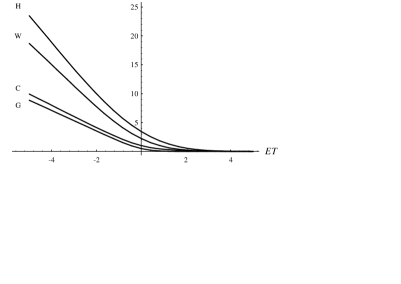
Figure 1: Vacuum response curves for switched detectors. The letters $G$, $C$, $W$ and $H$ denote Gaussian switching, Cauchy switching, Welch switching and Hanning switching, respectively.

Having explicitly illustrated the effects of excitation due to switching, from now on we shall consider the difference between the response in some given state $|A\rangle$ containing negative energy density or a negative energy flux and the vacuum $|0\rangle$:

$$\Delta\Pi_{A}(E;\vec{x}\,)=\Pi_{A}(E;\vec{x}\,)-\Pi_{0}(E;\vec{x}\,).$$ (23)

$\Delta\Pi_{A}$ will be finite even for sudden switching as the high frequency divergence is independent of state.

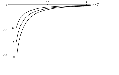
Figure 2: Response curves for energy $ET=1$ for a range of switched detectors a distance $z$ above a single Casimir plate. The letters $G$, $S$ and $H$ denote Gaussian switching, Sharp switching and Hanning switching, respectively.

To conclude this section we study a case of a static negative energy density before turning to negative energy fluxes in the next section. The simplest configuration to study is the field in its vacuum state $|{\rm Cas}\rangle$ outside a single Casimir plate $z=0$ on which the field is taken to vanish. For this configuration

$$\langle{\rm Cas}|\hat{\varphi}^{2}(z)|{\rm Cas}\rangle-\langle 0|\hat{\varphi}^{2}(z)|0\rangle=-{1\over 16\pi^{2}z^{2}},$$ (24)

which diverges to $-\infty$ as the plate is approached, and

$$\langle{\rm Cas}|\hat{\rho}_{\xi}(z)|{\rm Cas}\rangle-\langle 0|\hat{\rho}_{\xi}(z)|0\rangle=-{1\over 16\pi^{2}z^{4}}(1-6\xi).$$ (25)

In these equations $|0\rangle$ denotes the standard Minkowski vacuum. A calculation from Eq. (20) gives

$$\Delta\Pi_{\rm Cas}(E;z)=-{1\over 4\pi^{2}}\int\limits_{0}^{\infty}k{\rm d}k\>\bigl{|}\tilde{\lambda}(k+E)\bigr{|}^{2}\>{\sin(2kz)\over 2kz}$$

$$\ =-{1\over 4\pi^{2}}\int\limits_{0}^{\infty}w{\rm d}w\>\bigl{|}\tilde{\Lambda}(w+ET)\bigr{|}^{2}\>{\sin\left(2w(z/T)\right)\over 2w(z/T)}.$$ (26)

The response function $\Delta\Pi_{\rm Cas}(E,\vec{x}\,)$ is plotted for our range of switching functions in Fig. 2. It is clear from this that stimulated emission and absorption are reduced by the presence of the plate. This is a well known and experimentally observed effect. Note that as $\displaystyle{z/T}\to 0$, $\Delta\Pi_{\rm Cas}(E;z)\to-\Pi_{0}(E)$ since in this case the detector cannot become excited as can also be seen from Eq. (20) on noting that in this case $|f_{\vec{k}}(z\!=\!0)|=0$.

As a check on our calculations we may consider the response of an eternal detector by taking $\Lambda(\tau)=1$ $\forall\tau$, so $\tilde{\Lambda}(\omega)=2\pi\delta(\omega)$. In that case we find

$$\Delta\Pi_{\rm Cas}(E;z)=\begin{cases}0&E>0,\\ \displaystyle 2\pi\delta(0)\>{1\over 4\pi}{\sin(2Ez)\over z}&E<0,\\ \end{cases}$$ (27)

in agreement with the results of Ref. Davies:1989 for the response per unit time on identifying $2\pi\delta(0)$ as the total time of the measurement. As expected, in this case energy conservation prohibits excitation while de-excitation is affected by the presence of the mirror.

IV GENERAL STATE WITH ONE MODE EXCITED

A state of sufficient generality to illustrate the reponse of our switched detectors to negative energy fluxes is that of the most general state in which just a single mode of momentum $\vec{k}$ is excited. This may be written as

$$|\Psi\rangle=\sum\limits_{n=0}^{\infty}c_{n}|n\rangle,$$ (28)

where $|n\rangle$ denotes the $n$th excited state of the particular chosen mode and $\displaystyle\sum\limits_{n=0}^{\infty}|c_{n}|^{2}=1$. For simplicity we shall use a box normalization with box volume $V$. Without loss of generality we choose $\vec{k}=k\hat{x}$, then it is straightforward to calculate that

$$\langle\Psi|\hat{\varphi}(t,x)\hat{\varphi}(t^{\prime},x^{\prime})|\Psi\rangle-\langle 0|\hat{\varphi}(t,x)\hat{\varphi}(t^{\prime},x^{\prime})|0\rangle=$$

$${1\over kV}\biggl{\{}\cos k\bigl{(}(t-t^{\prime})-(x-x^{\prime})\bigr{)}\sum\limits_{n=0}^{\infty}n|c_{n}|^{2}+$$

$$\Re e\Bigl{[}{\rm e}^{-ik\left((t+t^{\prime})-(x+x^{\prime})\right)}\sum\limits_{n=2}^{\infty}\sqrt{n(n-1)}c_{n-2}^{\>*}c_{n}\Bigr{]}\biggr{\}},$$ (29)

where $\Re e$ denotes the real part. It follows that

$$\Delta\langle\hat{\varphi}^{2}\rangle={1\over kV}\biggl{\{}\sum\limits_{n=0}^{\infty}n|c_{n}|^{2}$$

$$\ {}+\Re e\Bigl{[}{\rm e}^{-i2k(t-x)}\sum\limits_{n=2}^{\infty}\sqrt{n(n-1)}c_{n-2}^{\>*}c_{n}\Bigr{]}\biggr{\}},$$ (30)

and

$$\Delta\langle\hat{\rho}_{\xi}\rangle=\Delta\langle\hat{F}_{\xi}\rangle={k\over V}\biggl{\{}\sum\limits_{n=0}^{\infty}n|c_{n}|^{2}$$

$$\ {}+(4\xi-1)\Re e\Bigl{[}{\rm e}^{-i2k(t-x)}\sum\limits_{n=2}^{\infty}\sqrt{n(n-1)}c_{n-2}^{\>*}c_{n}\Bigr{]}\biggr{\}}.$$ (31)

where ${\hat{\rho}}_{\xi}=-\hat{T}^{t}{}_{t}$ and $\hat{F}_{\xi}=\hat{T}^{x}{}_{t}$, are the energy density and right-moving energy flux respectively. All of these expressions correspond to the standard normal-ordered expectation values. The cross-terms here enable these quantities (which would classically be positive definite) to take either sign. The frequency of these cross terms is double that of the fundamental mode highlighting the interference nature of negative energy fluxes.

We now turn to our detector response. A straightforward calculation reveals

$$\Delta\Pi_{\Psi}(E;x)=$$

$${1\over 2kV}\biggl{\{}\Bigl{(}\bigl{|}\tilde{\Lambda}(kT+ET)\bigr{|}^{2}+\bigl{|}\tilde{\Lambda}(kT-ET)\bigr{|}^{2}\Bigr{)}\sum\limits_{n=0}^{\infty}n|c_{n}|^{2}$$

$${\qquad}+2\Re e\Bigl{[}\tilde{\Lambda}(kT+ET)\tilde{\Lambda}(kT-ET){\rm e}^{i2kx}$$

$${\qquad\qquad}\times\sum\limits_{n=2}^{\infty}\sqrt{n(n-1)}c_{n-2}^{\>*}c_{n}\Bigr{]}\biggr{\}}.$$ (32)

There are a number of observations to make about Eq. (32):

(a) $\Delta\Pi_{\Psi}(E,\vec{x}\,)$ is symmetric under $E\to-E$ as follows mathematically from the reality of the difference of the two Wightman functions and physically from the relationship between stimulated emission and absorption. In particular, although Grove’s discussion is expressed purely in terms of absorption, the approach here is entirely consistent with his results.

(b) It is easy to check that Eq. (16) holds for $\Delta\langle{\hat{\varphi}}^{2}\rangle$ of Eq. (30) and $\Delta\Pi_{\Psi}$ of Eq. (32) by virtue of Parseval’s theorem.

(c) For the special case of an $n$ particle state ($c_{n}=1$, all others zero) we have

$${\Delta\Pi}_{|n\rangle}(E;x)={n\over 2kV}\Bigl{\{}\bigl{|}\tilde{\Lambda}(ET+kT)\bigr{|}^{2}+\bigl{|}\tilde{\Lambda}(ET-kT)\bigr{|}^{2}\Bigr{\}}.$$ (33)

That the response is proportional to $n$ reassures us that in this simple case at least our switched monopole is acting as a particle detector.

(d)  Using the identity Ford:1991

$$\left(|\alpha|^{2}+|\beta|^{2}\right)\sum\limits_{n=0}^{\infty}n|c_{n}|^{2}$$

$$+2\Re e\left[\alpha\beta\sum\limits_{n=2}^{\infty}\sqrt{n(n-1)}c_{n-2}^{\>*}c_{n}\right]\geq-|\beta|^{2},$$ (34)

valid for arbitrary complex numbers $\alpha$, $\beta$ and $c_{n}$ such that $\displaystyle\sum\limits_{n=0}^{\infty}|c_{n}|^{2}=1$ we see that

$$\Delta\langle{\hat{\varphi}}^{2}\rangle\geq-{1\over kV}$$ (35)

and

$$\Delta\Pi_{\Psi}\geq-{1\over 2kV}\min\Bigl{(}\bigl{|}\tilde{\Lambda}(kT+ET)\bigr{|}^{2},\bigl{|}\tilde{\Lambda}(kT-ET)\bigr{|}^{2}\Bigr{)}.$$ (36)

Thus while either $\Delta\langle{\hat{\varphi}}^{2}\rangle$ or $\Delta\Pi_{\Psi}$ may be negative there is a limit as to how negative they can be. Eq. (35) is the direct analogue for $\langle{\hat{\varphi}}^{2}\rangle$ of the results obtained by Ford Ford:1991 for components of $\langle{\hat{\rho}}\rangle$. An interesting insight into Eq (36) is given by noting that

$${\Delta\Pi}_{|1\rangle}(E;x)={1\over 2kV}\Bigl{\{}\bigl{|}\tilde{\Lambda}(ET+kT)\bigr{|}^{2}+\bigl{|}\tilde{\Lambda}(ET-kT)\bigr{|}^{2}\Bigr{\}}$$

$$\quad\geq 2{1\over 2kV}\min\Bigl{(}\bigl{|}\tilde{\Lambda}(kT+ET)\bigr{|}^{2},\bigl{|}\tilde{\Lambda}(kT-ET)\bigr{|}^{2}\Bigr{)}.$$ (37)

so that

$$\Delta\Pi_{\Psi}\geq-\frac{1}{2}{\Delta\Pi}_{|1\rangle}(E;x).$$ (38)

This equation admits the following natural semi-classical interpretation. The detector may be thought to respond to the zero-point energy we have subtracted in forming $\Delta\Pi_{\Psi}$ exactly as an $n$-particle state with $n=\frac{1}{2}$. If we allow for the vacuum fluctuations in this way the total response will always be positive:

$$\Delta\Pi_{\Psi}+{\Delta\Pi}_{|-\frac{1}{2}\rangle}(E;x)\geq 0.$$ (39)

where ${\Delta\Pi}_{|-\frac{1}{2}\rangle}(E;x)$ is understood to be formally defined by Eq. (33) with $n=-\frac{1}{2}$.

A case of particular interest is that of (single mode) squeezed states defined for any complex number $\zeta$ by

$$|\zeta\rangle=\exp\left[{\textstyle{1\over 2}}\zeta^{*}{\hat{a}}^{2}-{\textstyle{1\over 2}}\zeta({\hat{a}}^{\dagger})^{2}\right]|0\rangle.$$ (40)

This state may be written in the present form with $c_{n}=0$ for $n$ odd and

$$c_{2n}=(\cosh r)^{-1/2}{\bigl{[}(2n)!\bigr{]}^{1/2}\over n!}\bigl{(}-{\textstyle{1\over 2}}{\rm e}^{i\theta}\tanh r\bigr{)}^{n},$$ (41)

where $\zeta=r{\rm e}^{i\theta}$. Correspondingly, we have

$$\Delta\langle\hat{\varphi}^{2}\rangle={1\over kV}\biggl{\{}\sinh^{2}r-\sinh r\cosh r\cos\bigl{[}2k(x-t)+\theta\bigr{]}\biggr{\}},$$ (42)

and

$$\Delta\langle\hat{\rho}_{\xi}\rangle=\Delta\langle\hat{F}_{\xi}\rangle={k\over V}\biggl{\{}\sinh^{2}r-$$

$$-(4\xi-1)\sinh r\cosh r\cos\bigl{[}2k(x-t)+\theta\bigr{]}\biggr{\}}.\qquad$$ (43)

Thus for a fraction $\cos^{-1}(\tanh r)/\pi$ of each cycle, $\Delta\langle\hat{\varphi}^{2}\rangle$ is negative; this is always less than half, tending to one half as $r$ tends to infinity. The average value of $\Delta\langle\hat{\varphi}^{2}\rangle$ over a cycle is $\sinh^{2}r/(kV)$ which is, of course, positive. For minimal coupling the energy density will be negative for an equal time but will be out of phase with $\Delta\langle\hat{\varphi}^{2}\rangle$. For other physical choices of couplings ($0<\xi\leq 1/6$), the energy density may or may not be negative depending on the degree of squeezing (magnitude of $r$). Whenever it is, it will always be out of phase with $\Delta\langle\hat{\varphi}^{2}\rangle$. The minimum value of $\Delta\langle\hat{\varphi}^{2}\rangle$ is

$$\Delta\langle\hat{\varphi}^{2}\rangle_{\rm min}=-{1\over kV}\{1-{\rm e}^{-2r}\},$$ (44)

which is, of course, consistent with the bound (35).

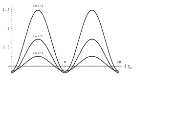
Figure 3: Response curves for squeezed states with squeezing factor $r={1\over 4}$, $r={1\over 2}$ and $r={3\over 4}$ for a detector with $\chi=1$.

The detector response to a squeezed state is given by

$${\Delta\Pi}_{\zeta}(E;x)=$$

$${1\over 2kV}\biggl{\{}\Bigl{(}\bigl{|}\tilde{\Lambda}(kT+ET)\bigr{|}^{2}+\bigl{|}\tilde{\Lambda}(kT-ET)\bigr{|}^{2}\Bigr{)}\sinh^{2}r$$

$$-2\sinh r\cosh r\ \Re e\Bigl{[}\tilde{\Lambda}(kT+ET)\tilde{\Lambda}(kT-ET){\rm e}^{i(2kx+\theta)}\Bigr{]}\biggl{\}},$$ (45)

or, equivalently,

$${\Delta\Pi}_{\zeta}(E;x)={1\over 2kV}\Bigl{(}\bigl{|}\tilde{\Lambda}(kT+ET)\bigr{|}^{2}+\bigl{|}\tilde{\Lambda}(kT-ET)\bigr{|}^{2}\Bigr{)}\times$$

$$\ \sinh r\cosh r\bigl{\{}\tanh r-\tanh\chi\cos{(2kx+\theta+\phi)}\bigr{\}},$$ (46)

where

$$\tanh\chi(kT,ET)\equiv{2\bigl{|}\tilde{\Lambda}(kT+ET)\bigr{|}\bigl{|}\tilde{\Lambda}(kT-ET)\bigr{|}\over\bigl{|}\tilde{\Lambda}(kT+ET)\bigr{|}^{2}+\bigl{|}\tilde{\Lambda}(kT-ET)\bigr{|}^{2}}$$ (47)

and $\phi\equiv{\rm Arg}\bigl{[}\tilde{\Lambda}(kT+ET)\tilde{\Lambda}(kT-ET)\bigr{]}$. For the switchings of Sec. II, which are all symmetric about $\tau=\tau_{0}$, we have $\phi=-2k\tau_{0}$.

It is clear from Eq.(46) that for fixed $kT$ and $ET$ there is a critical degree of squeezing, given by $0<|\zeta|=r<\chi$ required for the squeezed state to produce a suppression of vacuum excitation. For fixed $kT$ and $ET$ the minimum value attained by $\Delta\Pi_{\zeta}$ occurs for $r={1\over 2}\chi$, and in this case, one finds that for suitably chosen $x$ (or $\tau_{0}$) the lower bound (38) is achieved. Fig. 3 illustrates the response for $\chi=1$ as $k\tau_{0}$ is varied for $r={1\over 4}$, $r={1\over 2}$ and $r={3\over 4}$.

For sharp, Hanning and Welch switching the behaviour of $\tanh\chi(kT,ET)$ as a function of $kT$ and $ET$ is quite complicated; for illustration, $\tanh\chi_{S}(1,ET)$ for sharp switching is plotted as a function of $kE$ in Fig. 4. For Gaussian and Cauchy switching, $\tanh\chi$ is a monotonic decreasing function of $kT$ and $ET$. In the latter cases the explicit forms are sufficiently simple to be worth noting, we have

$$\tanh\chi_{G}=\operatorname{sech}(2kET^{2}),$$ (48)

and

$$\tanh\chi_{C}=\begin{cases}\operatorname{sech}(2ET)&ET<kT,\\ \operatorname{sech}(2kT)&ET\geq kT.\\ \end{cases}$$ (49)

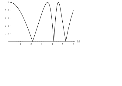
Figure 4: $\tanh\chi_{S}(kT,ET)$ for sharp switching plotted as a function of $kE$ for $kT=1$.

Another simple case in which there is a period of negative energy flux, which has been of historical importance, is that of the vacuum mixed with a two-particle state. In this case we have

$$|\Psi\rangle={1\over\surd(1+\epsilon^{2})}\bigl{(}|0\rangle+\epsilon|2\rangle\bigr{)},$$ (50)

where without loss of generality we have taken $\epsilon$ to be real. Corresponding to Eqs.(30) and (31) we have

$$\Delta\langle\hat{\varphi}^{2}\rangle={1\over kV}{1\over 1+\epsilon^{2}}\bigl{\{}2\epsilon^{2}+\sqrt{2}\epsilon\cos 2k(t-x)\bigr{\}}$$ (51)

and

$$\Delta \langle\hat{\rho}_{\xi}\rangle=\langle\hat{F}_{\xi}\rangle=$$

$$={k\over V}{1\over 1+\epsilon^{2}}\bigl{\{}2\epsilon^{2}+\sqrt{2}(4\xi-1)\epsilon\cos 2k(t-x)\bigr{\}}.$$ (52)

Clearly for small $\epsilon$ both $\Delta\langle\hat{\varphi}^{2}\rangle$ and $\Delta\langle\hat{\rho}_{\xi}\rangle$ can be negative for approximately half the time, and, as before, for physical choices of couplings ($0\leq\xi\leq 1/6$) these times are out of phase. Corresponding to Eq.(32) we have

$${\Delta\Pi}_{\Psi}(E;x)=$$

$$\quad{1\over 2\pi k(1+\epsilon^{2})}\biggl{\{}\epsilon^{2}\Bigl{(}\bigl{|}\tilde{\Lambda}(E+k)\bigr{|}^{2}+\bigl{|}\tilde{\Lambda}(E-k)\bigr{|}^{2}\Bigr{)}$$

$$\qquad+\Re e\Bigl{[}\sqrt{2}\epsilon\tilde{\Lambda}(kT+ET)\tilde{\Lambda}(kT-ET){\rm e}^{i2kx}\Bigr{]}\biggr{\}}$$

$$\quad={1\over 2\pi k(1+\epsilon^{2})}\Bigl{(}\bigl{|}\tilde{\Lambda}(E+k)\bigr{|}^{2}+\bigl{|}\tilde{\Lambda}(E-k)\bigr{|}^{2}\Bigr{)}\times$$

$$\qquad\qquad\Bigl{\{}\epsilon^{2}+{\epsilon\over\sqrt{2}}\tanh\chi\cos(2kx+\phi)\Bigr{\}}.$$ (53)

It is clear that for $\sqrt{2}|\epsilon|<\tanh\chi$ we will, as before, have periods when the excitation is less that in the vacuum.

We should add that the similarity of this case to that of squeezed states is not accidental: if we work only to order $\epsilon^{2}$ then the vacuum plus two particle state coincides with a squeezed state with $\zeta=-\sqrt{2}\epsilon$.

V RINDLER SPACE

Following Candelas and Sciama Candelas:1984 and Grove Grove:1988 , we will now study the response of an inertial detector moving through the Rindler vacuum, $|R\rangle$, defined in the wedge $x>|t|$ as illustrated in Fig. 5. The Rindler vacuum may be thought of as the natural vacuum state in the gravitational field of an infinite flat earth Sciama:1981 and is analogous to the Boulware vacuum of Schwarzschild space-time while the Minkowski vacuum is analogous to Hartle-Hawking vacuum. This scenario is thus related to the question posed by the title of Candelas and Sciama’s paper Candelas:1984 : ‘Is there a quantum equivalence principle?’ in which the authors addressed teh question of whether a detector falling freely in Schwarzschild space-time could distinguish if it was moving through the Hartle-Hawking vacuum or the Boulware vacuum.

An inertial detector moving through the Rindler vacuum must make a finite time measurement as the detector will reach the boundary of Rindler space in a finite proper time. This boundary plays the role of a mirror in that the field vanishes there; indeed the Rindler vacuum may be realised as the natural vacuum above a uniformly accelerating mirror in the limit that the acceleration tends to infinity.

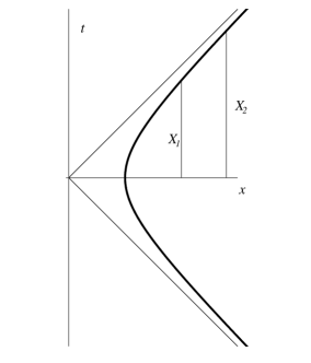
Figure 5: The measurement time of an inertial detector in Rindler space $x>|t|$ is limited by the presence of the boundary of Rindler space (mirror) at $x=t$. Candelas and Sciama chose to consider the limit $(X,T)\to\infty$ in such a way that the final acceleration $A=(X^{2}-T^{2})^{-1/2}$ remained constant as for the two trajectories marked $X_{1}$ and $X_{2}$ here.

Without loss of generality we may take the detector to be at fixed $x$, $x=X$ say. Then expressing the Rindler Wightman function in Minkowski coordinates we have

$$\langle R|\hat{\varphi}(t,X,y,z)\hat{\varphi}(t^{\prime},X,y,z)|R\rangle$$

$$\quad={1\over 2\pi^{2}(\eta^{2}-{\eta^{\prime}}^{2})}{\displaystyle\ln\left({\eta\over\eta^{\prime}}\right)\over\displaystyle\left[\ln^{2}\left({\eta\over\eta^{\prime}}\right)-(\tau-\tau^{\prime})^{2}\right]}$$

$$\quad={1\over 4\pi^{2}(t^{2}-{t^{\prime}}^{2})}\left[{1\over\displaystyle\ln\biggl{(}{X-t^{\prime}\over X-t}\biggr{)}}+{1\over\displaystyle\ln\biggl{(}{X+t^{\prime}\over X+t}\biggr{)}}\right],$$ (54)

where, as usual, $t=\eta\sinh\tau$ and $x=\eta\cosh\tau$. In Eq. (54) $t-t^{\prime}$ is understood to occur in the combination $t-t^{\prime}-i\epsilon$ appropriate to its character as a distribution.

For simplicity, we consider a detector switched on suddenly at $t=0$ and off suddenly at $t=T<X$. We have calculated the corresponding response $\Delta\Pi_{R}$ numerically. The result taking $X$ fixed and independent of $T$ is plotted in Fig. 6. That the response for fixed $E$ tends to $-\infty$ as $T\to X$ is to be expected on the basis of Eq. (16) since we have

$$\Delta\langle\hat{\varphi}^{2}(t)\rangle=-{1\over 48\pi^{2}\eta^{2}}=-{1\over 48\pi^{2}(X^{2}-t^{2})}$$ (55)

and so

$$\int\limits_{0}^{T}{\rm d}t\>\Delta\langle\hat{\varphi}^{2}(t)\rangle=-{1\over 96\pi^{2}X}\ln\left({X+T\over X-T}\right),$$ (56)

which diverges logarithmically to $-\infty$ as $T\to X$.

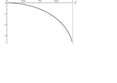
Figure 6: Detector response at energy $E=1$ for fixed $X=1$ as $T$ varies. $T=1$ corresponds to reaching the boundary of Rindler space.

Rather than consider the limit illustrated in Fig. 6, Candelas and Sciama chose to consider the limit $(X,T)\to\infty$ in such a way that the final acceleration $A=(X^{2}-T^{2})^{-1/2}$ remained constant. The numerically calculated detector response, $\Delta\Pi_{R}$, corresponding to this configuration is plotted in Fig. 7. The fact that this response tends to zero as $T\to\infty$ is the essence of the result obtained by Candelas and Sciama.

Both Figs. 6 and  7 bear out the conclusion of Grove that as a detector approaches the mirror the reduction in vacuum fluctuations near the mirror lead to a sharp reduction in the level of excitation of the detector. This interesting effect is lost in the limit taken by Candelas and Sciama.

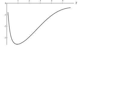
Figure 7: Detector response at energy $E=1$ as $T$ varies with $X$ varying so that the final acceleration $A=(X^{2}-T^{2})^{-1/2}$ is held fixed at $7{\cdot}09$ (so $X=1$ when $T=0{\cdot}99$).

In fact, as Candelas and Sciama did not subtract the infinite vacuum excitation introduced by their switching they were forced to consider the time derivative $\displaystyle{{\rm d}\over{\rm d}T}\Pi_{R}(E)$. This provides a notion of the difference in response between one ensemble of detectors switched on at time 0 and off at time $T$ and a different ensemble switched on at time 0 and off at time $T+{\rm d}T$. Grove considered $\displaystyle{{\rm d}\over{\rm d}T}\bigl{(}\Pi_{R}(E)-\Pi_{0}(E)\bigr{)}$ but incorrectly asserted that $\displaystyle{{\rm d}\over{\rm d}T}\Pi_{0}(E)=0$ whereas in reality

$${{\rm d}\over{\rm d}T}\Pi_{0}(E)={1\over 2\pi^{2}}\left[{\cos ET\over T}+E\,{\rm si}(ET)\right],$$ (57)

where ${\rm si}(x)$ is the sine integral defined by Gradsteyn:1980

$${\rm si}(x)\equiv\int\limits_{\infty}^{x}{\rm d}t\>{\sin t\over t}.$$

Eq. (57) may be derived either from differentiating Eq. (22) or directly by deforming the contour of integration to that used by Candelas and Sciama. Note that

$${{\rm d}\over{\rm d}T}\Pi_{0}(E)\to-{E\over 2\pi}\theta(-E)\qquad{\rm as}\quad T\to\infty$$ (58)

as required. Grove’s oversight does not in any case effect the analysis of the divergence in $\displaystyle{{\rm d}\over{\rm d}T}\Pi_{R}(E)$ as $T\to X$, since although $\displaystyle{{\rm d}\over{\rm d}T}\Pi_{0}(E)$ is non-vanishing it is manifestly regular in this limit. We shall work with $\displaystyle{{\rm d}\over{\rm d}T}\bigl{(}\Pi_{R}(E)-\Pi_{0}(E)\bigr{)}={{\rm d}\over{\rm d}T}\Delta\Pi_{R}(E)$ as this is more natural within our formalism.

Taking account of the foregoing comments, Candelas and Sciama prove that

$${{\rm d}\over{\rm d}T}\Delta\Pi_{R}(E)\sim- {1\over 8\pi^{2}}{\ln\bigl{|}2A^{2}T/E\bigr{|}\over T}$$

$$\qquad\text{as}\quad\bigl{|}A^{2}T/E\bigr{|}\to\infty.$$ (59)

From Eq. (16) we immediately obtain

$$\langle R|:\hat{\varphi}^{2}(T):|R\rangle={1\over 2\pi}\int\limits_{-\infty}^{\infty}{\rm d}E\>{{\rm d}\over{\rm d}T}\Delta\Pi_{R}(E).$$ (60)

We may follow Grove and use the asymptotic expression (59) of $\displaystyle{{\rm d}\over{\rm d}T}\Delta\Pi_{R}(E)$ for $\bigl{|}E/(2A^{2}T)\bigr{|}\leq{\cal O}(1)$ and approximate it as zero for $\bigl{|}E/(2A^{2}T)\bigr{|}>{\cal O}(1)$. Then

$${1\over 2\pi} \int\limits_{-\infty}^{\infty}{\rm d}E\>{{\rm d}\over{\rm d}T}\Delta\Pi_{R}(E)$$

$$\sim-{1\over 16\pi^{3}T}\int\limits_{-{\cal O}\bigl{(}2A^{2}T\bigr{)}}^{{\cal O}\bigl{(}2A^{2}T\bigr{)}}{\rm d}E\>\ln\bigl{|}E/(2A^{2}T)|$$

$$=-{A^{2}\over 4\pi^{3}}\int\limits_{0}^{{\cal O}(1)}{\rm d}x\>\ln x=-{A^{2}\over 4\pi^{3}}{\cal O}(1).$$ (61)

Given the crudeness of the calculation the agreement with the exact result

$$\langle R|:\hat{\varphi}^{2}(T):|R\rangle\sim-{A^{2}\over 48\pi^{2}}$$ (62)

is remarkable.

VI CONCLUSION

With our particular choice of linear coupling we have seen the very close link between detector response and reduced vacuum noise. The absence of vacuum fluctuations leads to a reduction in the level of excitations of a switched detector over that which would have occurred in the vacuum as a result of the switching. We may translate this into thermodynamic terms. We consider a hot ensemble of two level atoms which is initially at inverse temperature $\beta$ and is then allowed to interact for a finite time with a state $|\Psi\rangle$. The ensemble will, of course, cool (lose entropy) if it is placed just in the vacuum so we consider the change in entropy relative to the change in the vacuum which is given by

$$\Delta S={\beta E\over 1+{\rm e}^{-\beta E}}\bigl{[}\Delta\Pi_{\Psi}(E)-{\rm e}^{-\beta E}\Delta\Pi_{\Psi}(-E)\bigr{]}.$$ (63)

Considering for simplicity states for which $\Delta\Pi_{\Psi}(E)=\Delta\Pi_{\Psi}(-E)$ (for example, squeezed states) we have

$$\Delta S=\beta E\,{1-{\rm e}^{-\beta E}\over 1+{\rm e}^{-\beta E}}\,\Delta\Pi_{\Psi}(E).$$ (64)

Here the prefactor is manifestly positive so the ensemble which interacted with that state $|\Psi\rangle$ will have cooled more than an identical ensemble in the vacuum if and only if $\Delta\Pi_{\Psi}(E)<0$.

The foregoing results serve to clarify the response of matter to pulses of negative energy flux of limited duration. They are broadly in accordance with one’s intuition that negative energy should have the effect of enhancing de-excitation, i.e. to induce ‘cooling’. However, our results are necessarily somewhat model dependent and for our standard monopole model we find that there is not always a simple relationship between the strength of the negative energy flux and the behaviour of matter.

Considerable interest attaches to the thermodynamics of negative energy. If a sustained negative energy flux could be directed at a hot body (or a black hole) in such a way as to reduce its temperature, hence entropy, by a macroscopic amount there would appear to be a clear violation of the second law of thermodynamics. There is a considerable literature on this topic already. The results of this paper are a first step to investigating the thermodynamics of negative energy. However, the ‘cooling’ effects we have discussed cannot be immediately used to draw thermodynamic conclusions, because they have been restricted to first order in perturbation theory and, as shown by Grove Grove:1986 , a proper investigation of the thermodynamic implications necessitates a calculation to second order in perturbation theory. (At first order alone, it is not possible to determine whether the de-excitation effects are merely due to the (small) violation of energy conservation expected in any process in which a general quantum state collapses to an energy eigenstate, or whether they pressage a systematic reduction in the energy of the matter which would have serious thermodynamic implications.) We shall report on this further investigation in a separate paper.

References

- (1) H. Epstein, V. Glaser and A. Jaffe, Nuovo Cimento 36, 1016 (1965)
- (2) M. Morris and K. Thorne, Am.J.Phys. 56, 395 (1988)
- (3) M. Morris, K. Thorne and Y. Yurtsever, Phys.Rev.Lett.61, 1446 (1988)
- (4) L.H. Ford and T.A. Roman, Phys.Rev. D41 3662 (1990)
- (5) L.H. Ford and T.A. Roman, Phys.Rev. D46 1328 (1992)
- (6) L.H. Ford, Proc.R.Soc.(London) A346, 227 (1978)
- (7) P.C.W. Davies, Phys.Lett.113B, 393 (1982)
- (8) L.H. Ford, Phys.Rev.D43, 3972 (1991)
- (9) L.H. Ford and T.A. Roman, Phys.Rev. D51 4277 (1995)
- (10) L.H. Ford and T.A. Roman, Phys.Rev. D55 2082 (1997)
- (11) M.J. Pfenning and L. H. Ford Phys.Rev. D57 3489 (1998)
- (12) L.H. Ford, M.J. Pfenning and T.A. Roman, Phys.Rev. D57 4839 (1998)
- (13) C. Fewster and S. Eveson, Phys.Rev. D58 084010 (1998)
- (14) C. Fewster and E. Teo, Phys.Rev. D59 104016 (1999)
- (15) É.É. Flanagan, Phys.Rev. D56 4922 (1997)
- (16) P.G. Grove, Class. Quantum Grav.5, 1381 (1988)
- (17) L.H. Ford, P.G. Grove and A.C. Ottewill, Phys.Rev. D46 4566 (1992)
- (18) A.D. Helfer, Class. Quantum Grav. 15, 1169 (1998)
- (19) P. Candelas and D.W. Sciama, Phys. Rev.D27, 1715 (1983) ; also published in Quantum Theory of Gravity, ed. S.M. Christensen (Adam Hilger, Bristol, 1984)) p.78
- (20) C.W. Misner, K.S. Thorne and J.A. Wheeler, Gravitation (Freeman, San Francisco, 1973)
- (21) E.J. Hannon, Multiple Time Series (Wiley, New York, 1970)
- (22) P.C.W. Davies, Z.X. Liu and A.C. Ottewill, Class. Quantum Grav. 6, 1041 (1989)
- (23) P.G. Grove, Class. Quantum Grav.3, 801 (1986)
- (24) I.S. Gradsteyn and I.M. Ryzhik, Tables of Integrals, Series and Products (Academic Press, New York, 1980)
- (25) D.W. Sciama, P. Candelas and D. Deutsch, Adv. Phys. 30, 327 (1981)