Background of gravitational waves from pre-galactic black hole formation

Abstract

We study the generation of a gravitational wave (GW) background produced from a population of core-collapse supernovae, which form black holes in scenarios of structure formation of the Universe. We obtain, for example, that a pre-galactic population of black holes, formed at redshifts $z\simeq 30-10$, could generate a stochastic GW background with a maximum amplitude of $h_{\rm BG}\simeq 10^{-24}$ in the frequency band $\nu_{\rm obs}\simeq 30-470{\rm Hz}$ (considering a maximum efficiency of generation of GWs, namely, $\varepsilon_{\rm GW}=7\times 10^{-4}$). In particular, we discuss what astrophysical information could be obtained from a positive, or even a negative, detection of such a GW background produced in scenarios such as those studied here. One of them is the possibility of obtaining the initial and final redshifts of the emission period from the observed spectrum of GWs.

1 Introduction

Because of the fact that gravitational waves (GWs) are produced by a large variety of astrophysical sources and cosmological phenomena, it is quite probable that the Universe is pervaded by a background of such waves. A variety of binary stars (ordinary, compact or combinations of them), Population III stars, phase transitions in the early Universe and cosmic strings are examples of sources that could produce such a putative background of GWs (Thorne 1987, Blair and Ju 1996, Owen et al1998, Ferrari et al1999a, 1999b, Schutz 1999, Giovannini 2000, Maggiore 2000, Schneider et al2000, among others).

In the present study we have considered the background of GWs produced from a Population III black hole formation. The basic arguments in favour of the existence of these pre-galactic black holes are the following: (a) from the Gunn-Peterson effect (Gunn and Peterson 1965), it is widely accepted that the Universe underwent a reheating (or reionization) phase between the standard recombination epoch (at $z\sim 1000$) and $z>5$ as a result of the formation of the first structures of the Universe (see, Haiman and Loeb 1997, Loeb and Barkana 2001 for a review). However, at what redshift the reionization occured is still an open question (Loeb and Barkana 2001), although recent studies conclude that it occurred at redshifts in the range $6<z<30$ (Venkatesan 2000); (b) the metallicity of $\sim 10^{-2}Z_{\odot}$ found in ${\rm high}-z$ Ly$\alpha$ forest clouds (Songaila and Cowie 1996, Ellison et al2000) is consistent with a stellar population formed at $z>5$ (Venkatesan 2000).

In the present paper we have adopted a stellar generation with a Salpeter initial mass function (IMF) as well as different stellar formation epochs. We then discuss what conclusions would be drawn from whether (or not) the stochastic background studied here is detected by forthcoming GW observatories such as LIGO and VIRGO.

The paper is organized as follows. In section 2 we describe how to calculate the background of GWs produced during the formation of the stellar black holes in this scenario (the reader finds a more detailed description in de Araujo et al2002), in section 3 we present some numerical results and the discussions, in section 4 we consider the detectability of this putative GW background and finally in section 5 we present our conclusions.

2 The gravitational wave production from pre-galactic stars

Before going into detail of the calculation of the background of GWs produced by pre-galactic stars, it is import to consider in what ways the present study differs from previous ones.

Ferrari et al(1999a), for example, consider the background of GWs produced by the formation of black holes of galactic origin, i.e., those formed at redshifts $z<5$. Schneider et al(2000) study the collapse of Very Massive Objects (VMO), and the eventual formation of very massive black holes and the GWs they generate. Fryer et al(2002) study, among other issues, the collapse of very massive Population III stars ($>300{\rm M}_{\odot}$) and the GWs generated by them.

Here, we consider a different approach to the formation of pre-galactic objects. We take into account the formation of Population III stellar black holes, considering that the progenitor stars follow a Salpeter’s IMF. In this case, the progenitor stars have masses in the range $25-125M_{\odot}$. We also consider that the formation of these black holes occurs at high redshifts, namely, $z>10$. It is worth noting that Sapeter’s Population III stars could account for the metallicity found in high-z Ly$\alpha$ forest clouds, and, at least in part, since the QSOs could also be important, for the reionization of the Universe.

Let us now focus on how to calculate the background of GWs produced by the Population III stellar black holes we propose exist.

The spectral energy density, the flux of GWs, received on Earth, $F_{\nu}$, in ${\rm erg}\,{\rm cm}^{-2}\,{\rm s}^{-1}\,{\rm Hz}^{-1}$, reads (see, e.g. Douglass and Braginsky 1979, Hils et al1990)

$$F_{\nu}={c^{3}s_{\rm h}\omega_{\rm obs}^{2}\over 16{\rm\pi}G},$$ (1)

where $\omega_{\rm obs}=2{\rm\pi}\nu_{\rm{obs}}$, with $\nu_{\rm{obs}}$ being the GW frequency (Hz) observed on Earth, $c$ is the velocity of light, $G$ is the gravitational constant and $\sqrt{s_{\rm h}}$ is the strain amplitude of the GW ($\rm Hz^{-1/2}$).

The stochastic GW background produced by gravitational collapses that lead to black holes would have a spectral density of the flux of GWs and strain amplitude also related to equation (1). The strain amplitude at a given frequency, at the present time, is the contribution of black holes with different masses at different redshifts. Thus, the ensemble of black holes formed produces a background whose characteristic strain amplitude at the present time is $\sqrt{s}_{\rm h}$.

On the other hand, the spectral density of the flux can be written as (Ferrari et al1999a)

$$F_{\nu}=\int_{z_{\rm{cf}}}^{z_{\rm{ci}}}\int_{m_{\rm{min}}}^{m_{\rm{u}}}f_{\nu}(\nu_{\rm{obs}})dR_{\rm BH}(m,z)$$ (2)

where $f_{\nu}(\nu_{\rm{obs}})$ is the energy flux per unit of frequency (in ${\rm erg}\,{\rm cm}^{-2}\,{\rm Hz}^{-1}$) produced due to the formation of a unique black hole and $dR_{\rm BH}$ is the differential rate of black hole formation.

The above equation takes into account the contribution of different masses that collapse to form black holes occurring between redshifts $z_{\rm ci}$ and $z_{\rm cf}$ (beginning and end of the star formation phase, respectively) that produce a signal at the same frequency $\nu_{\rm{obs}}$. On the other hand, we can write $f_{\nu}(\nu_{\rm{obs}})$ (Carr 1980) as

$$f_{\nu}(\nu_{\rm{obs}})={{\rm\pi}c^{3}\over 2G}h_{\rm BH}^{2}$$ (3)

where $h_{\rm BH}$ is the dimensionless amplitude produced by the collapse, to a black hole, of a given star with mass $m$ that generates at the present time a signal with frequency $\nu_{\rm{obs}}$. Then, the resulting equation for the spectral density of the flux is

$$F_{\nu}={\pi c^{3}\over 2G}\int h_{\rm BH}^{2}dR_{\rm BH}.$$ (4)

From the above equations, we obtain for the strain amplitude

$$s_{\rm h}={1\over\nu_{\rm obs}^{2}}\int h_{\rm BH}^{2}dR_{\rm BH}.$$ (5)

Then, the dimensionless amplitude of the background of GWs, $h_{\rm BG}$, reads

$$h_{\rm BG}^{2}={1\over\nu_{\rm obs}}\int h_{\rm BH}^{2}dR_{\rm BH}$$ (6)

(see, de Araujo et al2000 for details) where $\nu_{\rm obs}$, $h_{\rm BH}$ and $dR_{\rm BH}$ are defined below.

The dimensionless amplitude $h_{\rm BH}$ produced by the collapse of a star, or star cluster, to form a black hole is (Thorne 1987)

$$h_{\rm BH}\simeq 7.4\times 10^{-20}\,\varepsilon_{\rm GW}^{1/2}\bigg{(}{M_{\rm r}\over{\bf M}_{\odot}}\bigg{)}\bigg{(}{d_{\rm L}\over 1{\rm Mpc}}\bigg{)}^{-1}$$ (7)

where $\varepsilon_{\rm GW}$ is the efficiency of generation of GWs, $M_{\rm r}$ is the remnant black hole mass and $d_{\rm L}$ is the luminosity distance to the source.

It is worth mentioning that equation (7) refers to the black hole ‘ringing’, which has to do with the de-excitation of the black hole quasi-normal modes. Note also that $\varepsilon_{\rm GW}\propto a^{4}$ (see, e.g. Stark and Piran 1986), where ‘$a$’ is the the dimensionless angular momentum. Thus, greater the GW efficiency, greater the dimensionless angular momentum.

We assume that the progenitor masses of the black holes range from $M=25-125{\rm M}_{\odot}$ (see Timmes et al1995, Woosley and Timmes 1996). The remnant and the progenitor masses are related to $M_{\rm r}=\alpha M$ and, we assume $\alpha=0.1$ (see, e.g. Ferrari et al1999a).

The collapse of a star to a black hole produces a signal with an observed frequency $\nu_{\rm{obs}}$ at the Earth (Thorne 1987)

$$\nu_{\rm{obs}}\simeq 1.3\times 10^{4}\,{\rm Hz}\bigg{(}{{\rm M}_{\odot}\over M_{\rm r}}\bigg{)}(1+z)^{-1}$$ (8)

where the factor $(1+z)^{-1}$ takes into account the redshift effect on the emission frequency.

The differential rate of black hole formation $dR_{\rm BH}$ reads

$$dR_{\rm BH}=\dot{\rho}_{\star}(z){dV\over dz}\phi(m)dmdz$$ (9)

where $dV$ is the co-moving volume element, $\phi(m)$ is the stellar initial mass function (IMF) and $\dot{\rho}_{\star}(z)$ is the star formation rate (SFR) density.

The SFR density can be related to the reionization of the Universe. The amount of baryons necessary to participate in early star formation, to account for the reionization, would amount to a small fraction, $f_{\star}$, of all baryons of the Universe (see, e.g. Loeb and Barkana 2001). We then assume that

$$\dot{\rho}_{\star}\equiv{d\rho_{\star}\over dt}={d\over dt}[\Omega_{\star}\;\rho_{\rm c}\;(1+z)^{3}]$$ (10)

where the term in brackets represents the stellar mass density at redshift $z$, with $\rho_{\rm c}$ the present critical density, and $\Omega_{\star}$ the stellar density parameter. The latter can be written as a fraction of the baryonic density parameter, namely, $\Omega_{\star}=f_{\star}\Omega_{\rm B}$, which we assume to be independent of the redshift.

From the above equations, we obtain for the dimensionless amplitude

$$h_{\rm BG}^{2} = {(7.4\times 10^{-20}\alpha)^{2}\varepsilon_{\rm GW}\over\nu_{\rm{obs}}}$$ (11)

$$\times\bigg{[}\int_{z_{\rm cf}}^{z_{\rm ci}}\int_{m_{\rm min}}^{m_{\rm u}}\bigg{(}{m\over{\rm M}_{\odot}}\bigg{)}^{2}\bigg{(}{d_{\rm L}\over 1{\rm Mpc}}\bigg{)}^{-2}\dot{\rho}_{\star}(z){dV\over dz}\phi(m)dmdz\bigg{]}$$

where $m_{\rm min}=25{\rm M}_{\odot}$, $m_{\rm u}=125{\rm M}_{\odot}$ and $z_{\rm ci}$ ($z_{\rm cf}$) is the beginning (end) of the black hole formation phase. Equation (11) is computed for each observed frequency. Also, looking at equation (11), one notes that to integrate it, one needs to choose the IMF, the cosmological parameters and set values for the following parameters: $z_{\rm ci}$, $z_{\rm cf}$, $\alpha$, $\varepsilon_{\rm GW}$, $f_{\star}$. In the next section we present the numerical results and discussions.

3 Numerical results and discussions

To evaluate the background of GWs produced by the formation of the Population III black holes, it is necessary to know in which redshifts they began and finished formation. This is a very difficult question to answer, since it involves knowledge of the role of the negative and positive feedbacks of star formation which are regulated by cooling and injection of energy processes.

Should the stochastic background of GWs studied here be significantly produced and detected at a reasonable confidence level, the present study can be used to obtain the redshift range where the Population III black holes were formed. We refer the reader to the paper by de Araujo et al(2002) for further discussions. In figure 1 an example is given of how one could get $z_{\rm ci}$ and $z_{\rm cf}$ from the curve $h_{\rm BG}$ versus $\nu_{\rm obs}$. Knowing the frequency band $\nu_{\rm min}-\nu_{\rm max}$ detected from a cosmological source, and using equation (8), one can obtain both $z_{\rm ci}$ and $z_{\rm cf}$ from figure 1. Thus, these redshifts are therefore observable. Note that we have assumed as did Ferrari et al(1999a) that $\alpha$ is a constant ($\alpha=0.1$).

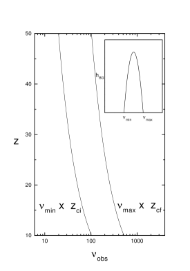
Figure 1: Example of how one could obtain the initial (final) redshift $z_{\rm ci}$ ($z_{\rm cf}$) of the GW emission period from $h_{\rm BG}$ versus $\nu_{\rm obs}$. We have adopted $\alpha=0.1$.

Stars start forming at different redshifts, creating ionized bubbles (Strömgren spheres) around themselves, which expand into the intergalactic medium (IGM), at a rate dictated by the source luminosity and the background IGM density (Loeb and Barkana 2001). The reionization is complete when the bubbles overlap to fill the entire Universe. Thus the epoch of reionization is not the epoch of star formation. There is a non-negligible time span between them. Here, we have chosen different formation epochs to see their influence on the putative background of GWs and also to see if it could be detected by the forthcoming GW antennas.

To calculate $h_{\rm BG}$ we adopted the standard Salpeter IMF. For $\varepsilon_{\rm GW}$, the efficiency of production of GWs, whose distribution function is unknown, we have parametrized our results in terms of its maximum value, namely, $\varepsilon_{\rm GW_{\rm max}}=7\times 10^{-4}$. This figure is obtained from studies by Stark and Piran (1986) who simulated the axisymmetric collapse of a rotating star to a black hole.

To calculate $h_{\rm BG}$ we still need to know $\Omega_{\star}$, which has a key role in the definition of the SFR density. From different studies one can conclude that a few per cent, may be up to $\sim 10\%$, of the baryons must be condensed into stars in order for the reionization of the Universe to take place (see, e.g. Venkatesan 2000). Here we have set the value of $\Omega_{\star}$ in such a way that it amounts to $1\%$ of all baryons (our fiducial value).

Looking at equation (11), one could think it would depend critically on the cosmological parameters $H_{0}$, $\Omega_{\rm B}$, $\Omega_{\rm DM}$ (the density parameter for the dark matter) and $\Omega_{\Lambda}$ (the density parameter associated with the cosmological constant). But our results show that $h_{\rm BG}$ depends only on $H_{0}$ and $\Omega_{\rm B}$, the Hubble parameter and the baryonic density parameter, respectively.

The quantity $h_{100}^{2}\Omega_{\rm B}=0.019\pm 0.0024$ (where $h_{100}$ is the Hubble parameter given in terms of 100 ${\rm km\;s^{-1}\;Mpc^{-1}}$) is adopted in the present model. This figure is obtained from Big Bang nucleosynthesis studies (see, e.g. Burles et al1999).

In table 1 we present the redshift band, $z_{\rm ci}$ and $z_{\rm cf}$, for the models studied and the corresponding GW frequency bands. For the cosmological parameters, we have adopted $h_{100}=0.65$, $\Omega_{\rm M}=0.3$, $\Omega_{\rm B}=0.045$ and $\Omega_{\Lambda}=0.7$. We have also adopted $\alpha=0.1$, $f_{\star}=0.01$ and the standard IMF.

It is worth noting that no structure formation model has been used to find the black holes formation epoch; instead, we have simply chosen the values of $z$ to see whether it is possible to obtain detectable GW signals. In the next section, it will be seen that unless $\varepsilon_{\rm GW}$ is negligible, the background of GWs we propose here can be detected. Our choices, however, can be understood as follows. The greater the redshift formation, the more power the masses related to the Population III objects have. Thus from our models A to D, our model D (A) has more (less) power when compared to the others. The models E, F and G would mean a more extended star formation epoch, which means that the feedback processes of star formation are such that they allow a more extended star formation epoch when compared to the models B, C and D, respectively.

Note that the reionization epoch occurred at lower redshifts as compared to the first stars formation redshifts. Loeb and Barkana (2001) found, for example, that if the stars were formed at $z\simeq 10-30$, with standard IMF, they could have reionized the Universe at redshift $z\sim 6$. Our models A, B and E, for example, could account for such a reionization redshift.

If the process of structure formation of the Universe and the consequent star formation were well known, one could obtain the redshift formation epoch of the first stars. On the other hand, if the background of GWs really exists and is detected, one can obtain information about the formation epoch of the first stars.

Table 1: The redshifts of collapse for our models and the corresponding GW frequency bands. The cosmological parameter $h_{100}^{2}\Omega_{\rm B}=0.019$ (see the text), $\alpha=0.1$, $f_{\star}=0.01$ (our fiducial value) and the standard IMF are adopted.

• Model	$z_{\rm ci}$	$z_{\rm cf}$	$\Delta\nu_{\rm obs}$ (Hz)
  A	20	10	50-470
  B	30	20	34-250
  C	40	30	25-170
  D	50	40	20-130
  E	30	10	34-470
  F	40	10	25-470
  G	50	10	20-470

A relevant question is whether the background we study here is continuous or not. The duty cycle indicates if the collective effect of the bursts of GWs generated during the collapse of a progenitor star generates a continuous background. For all the models studied here the duty cycle is $\gg 1$ (see de Araujo et al2002 for details).

We find, for example, that the formation of a Population (III) of black holes, in the model D, could generate a stochastic background of GWs with amplitude $h_{\rm BG}\simeq(0.8-2)\times 10^{-24}$ and a corresponding closure density of $\Omega_{\rm{GW}}\simeq(0.7-1.4)\times 10^{-8}$, at the frequency band $\nu_{\rm{obs}}\simeq 20-130\,{\rm Hz}$ (assuming an efficiency of generation $\varepsilon_{\rm GW}\simeq 7\times 10^{-4}$, the maximum one).

In other paper to appear elsewhere (de Araujo et al2002), we study in detail how the variations of the several parameters modify our results.

4 Detectability of the background of gravitational waves

The background predicted in the present study cannot be detected by single forthcoming interferometric detectors, such as VIRGO and LIGO (even by advanced ones). However, it is possible to correlate the signal of two or more detectors to detect the background that we propose to exist.

To assess the detectability of a GW signal, one must evaluate the signal-to-noise ratio (SNR), which for a pair of interferometers is given by (see, e.g. Flanagan 1993)

$${\rm SNR}^{2}=\left[\left(\frac{9H_{0}^{4}}{50\pi^{4}}\right)T\int_{0}^{\infty}d\nu\frac{\gamma^{2}(\nu)\Omega^{2}_{GW}(\nu)}{\nu^{6}S_{\rm h}^{(1)}(\nu)S_{\rm h}^{(2)}(\nu)}\right]$$ (12)

where $S_{\rm h}^{(i)}$ is the spectral noise density, $T$ is the integration time and $\gamma(\nu)$ is the overlap reduction function, which depends on the relative positions and orientations of the two interferometers. The closure energy density is given by

$$\Omega_{\rm GW}={1\over\rho_{\rm c}}{d\rho_{\rm GW}\over d\log\nu_{\rm{obs}}}={4{\rm\pi}^{2}\over 3H^{2}_{0}}\nu_{\rm{obs}}^{2}h_{\rm BG}^{2}.$$ (13)

Here we consider, in particular, the LIGO interferometers, and their spectral noise densities have been taken from a paper by Owen et al(1998).

In table 2 we present the SNR for 1 year of observation with $\alpha=0.1$, $\Omega_{\rm B}h^{2}_{100}=0.019$, $f_{\star}=0.01$ and $\varepsilon_{\rm GW_{\rm max}}=7\times 10^{-4}$ for the models in table 1, for the three LIGO interferometer configurations.

Table 2: For the models in table 1, we present the SNR for pairs of LIGO I, II and III (‘first’, ‘enhanced’ and ‘advanced’, respectively) observatories for 1 year of observation. Note that an efficiency of generation $\varepsilon_{\rm GW_{\rm max}}=7\times 10^{-4}$ is assumed.

• 		SNR
  Model	LIGO I	LIGO II	LIGO III
  A	$8.3\times 10^{-3}$	$1.6$	$6.6$
  B	$8.5\times 10^{-3}$	$2.3$	$26$
  C	$8.7\times 10^{-3}$	$2.7$	$47$
  D	$8.1\times 10^{-3}$	$2.5$	$51$
  E	$2.7\times 10^{-3}$	$5.7$	$37$
  F	$5.0\times 10^{-3}$	$12$	$120$
  G	$7.7\times 10^{-2}$	$21$	$260$

Note that for the ‘initial’ LIGO (LIGO I), there is no hope of detecting the background of GWs we propose here. For the ‘enhanced’ LIGO (LIGO II) there is some possibility of detecting the background, since ${\rm SNR}>1$, if $\varepsilon_{\rm GW}$ is around the maximum value. Even if the LIGO II interferometers cannot detect such a background, it will be possible to constrain the efficiency of GW production.

The prospect of detection with the ‘advanced’ LIGO (LIGO III) interferometers is much more optimistic, since the SNR for almost all models is significantly greater than unity. Only if the value of $\varepsilon_{\rm GW}$ were significantly lower than the maximum value would the detection not be possible. In fact, the signal-to-noise ratio is critically dependent on this parameter.

Note that the larger the star formation redshift band, the greater the SNR. Secondly, the earlier the star formation, the greater the SNR. It is worth recalling that, if one can obtain the curve ‘$h_{\rm BG}$ versus $\nu_{\rm obs}$’ and the value of $\alpha$ is known, one can find the redshift of star formation.

5 Conclusions

We have shown that a background of GWs is produced from Population III black hole formation at high redshift. This background can in principle be detected by a pair of LIGO II (or more probably by a pair of LIGO III) interferometers. However, a relevant question should be considered: what astrophysical information can one obtain whether or not such a putative background is detected?

First, let us consider a non-detection of the GW background. The critical parameter to be constrained here is $\varepsilon_{\rm GW}$. A non-detection would mean that the efficiency of GWs during the formation of black holes is not high enough. Another possibility is that the first generation of stars is such that the black holes formed had masses $>100M_{\odot}$, and should they form at $z>10$ the GW frequency band would be out of the LIGO frequency band.

Secondly, a detection of the background with a significant SNR would permit us to obtain the curve of $h_{\rm BG}$ versus $\nu_{\rm obs}$. From it, one can constrain $\alpha$ and the redshift formation epoch; and for a given IMF and $\Omega_{\rm B}h^{2}$, one can also constrain the values of $f_{\star}$ and $\varepsilon_{\rm GW}$. On the other hand, using the curve of $h_{\rm BG}$ versus $\nu_{\rm obs}$ and in addition other astrophysical data, say CBR data, models of structure formation and reionization of the Universe, constraint on $\varepsilon_{\rm GW}$ can also be imposed. We refer the reader to the paper by de Araujo et al(2002) for further discussions.

It is worth mentioning that a significant amount of GWs can also be produced during the formation of neutron stars and if such stars are r-mode unstable (Andersson 1998). We leave these issues for other studies to appear elsewhere.

References

References

- [1]
- [2] []Andersson N 1998 Astrophys. J. 211 708
- [3]
- [4] []Blair D G and Ju L 1996 Mon. Not. R. Astron. Soc. 283 618
- [5]
- [6] []Burles S, Nollett K M, Truran J N and Turner M S 1999 Phys.Rev.Lett. 82 4176
- [7]
- [8] []Carr B J 1980 Astron. Astrophys. 89 6
- [9]
- [10] []de Araujo J C N, Miranda O D and Aguiar O D 2000 Phys. Rev. D 61 124015
- [11]
- [12] []de Araujo J C N, Miranda O D and Aguiar O D 2002 Mon. Not. R. Astron. Soc. at press
- [13]
- [14] []Douglass D H and Braginsky V G 1979 General Relativity: An Einstein Centenary Survey (Cambridge: Cambridge University Press) p 90
- [15]
- [16] []Ellison S, Songaila A, Schaye J and Petinni M 2000 Astron. J. 120 1175
- [17]
- [18] []Ferrari V, Matarrese S and Schneider R 1999a Mon. Not. R. Astron. Soc. 303 247
- [19]
- [20] []Ferrari V, Matarrese S and Schneider R 1999b Mon. Not. R. Astron. Soc. 303 258
- [21]
- [22] []Flanagan E E 1993 Phys. Rev. D 48 2389
- [23]
- [24] [] Fryer C L, Holz D E and Hughes S A 2002 Astrophys. J. 565 430
- [25]
- [26] []Giovannini M 2000 Preprint gr-qc/0009101
- [27]
- [28] [] Gunn J E and Peterson B A 1965 Astrophys. J. 142 1633
- [29]
- [30] []Haiman Z and Loeb A 1997 Astrophys. J. 483 21
- [31]
- [32] []Hils D, Bender P L and Webbink R F 1990 Astrophys. J. 360 75
- [33]
- [34] []Loeb A and Barkana R 2001 Ann. Rev. Astron. Astrophys. 39 19
- [35]
- [36] []Maggiore M 2000 Phys. Rep. 331 283
- [37]
- [38] []Owen B J, Lindblom L, Cutler C, Schutz B F, Vecchio A and Andersson N 1998 Phys. Rev. D 58 084020
- [39]
- [40] []Schneider R, Ferrara A, Ciardi B, Ferrari V and Matarrese S 2000 Mon. Not. R. Astron. Soc. 317 385
- [41]
- [42] []Schutz B F 1999 Class. Quantum Grav. 16 A131
- [43]
- [44] []Songaila A and Cowie L L 1996 Astron. J. 112 335
- [45]
- [46] []Stark R F and Piran T 1986 Proc. 4th Marcel Grossmann Meeting on General Relativity (Rome, Italy) (Amsterdam: Elsevier) p 327
- [47]
- [48] []Thorne K S 1987 300 years of Gravitation (Cambridge: Cambridge University Press) p 331
- [49]
- [50] [] Timmes F X, Woosley S E and Weaver T A 1995 Astrophys. J. Suppl 98 617
- [51]
- [52] []Venkatesan A 2000 Astrophys. J. 537 55
- [53]
- [54] Woosley S E and Timmes F X 1996 Nucl. Phys. A 606 137
- [55]