The detection of Gravitational Waves

Abstract

This chapter is concerned with the question: how do gravitational waves (GWs) interact with their detectors? It is intended to be a theoretical review of the fundamental concepts involved in interferometric and acoustic (Weber bar) GW antennas. In particular, the type of signal the GW deposits in the detector in each case will be assessed, as well as its intensity and deconvolution. Brief reference will also be made to detector sensitivity characterisation, including very summary data on current state of the art GW detectors.

1 Introduction

Gravitational waves (GW), on very general grounds, appear to be a largely unavoidable consequence of a well established fact that no known interaction propagates instantly from source to observer: gravitation would be the first exception to this rule, should it be described by Newton’s theory. Indeed, the Newtonian gravitational potential $\phi(\vec{x},t)$ satisfies Poisson’s equation

$$\nabla^{2}\phi(\vec{x},t)=-4\pi G\,\varrho(\vec{x},t)\;,$$ (1)

where $\varrho(\vec{x},t)$ is the density of matter in the sources of gravitational fields, and $G\/$ is Newton’s constant. But, since (1) contains no time derivatives, the time dependence of $\phi(\vec{x},t)$ is purely parametric, i.e., time variations in $\varrho(\vec{x},t)$ instantly carry over to $\phi(\vec{x},t)$, irrespective of the value of $\vec{x}$. So, for example, non-spherically symmetric fluctuations in the mass distribution of the Sun (such as e.g. those caused by solar storms) would instantly and simultaneously be felt both in the nearby Mercury and in the remote Pluto…

Quite independently of the quantitative relevance of such instant propagation effect in this particular example – which is none in practice –, its very existence is conceptually distressing. In addition, the asymmetry between the space and time variables in (1) does not even comply with the basic requirements of Special Relativity.

Einstein’s solution to the problem of gravity, General Relativity (GR), does indeed predict the existence of radiation of gravitational waves. As early as 1918, Einstein himself provided a full description of the polarisation and propagation properties of weak GWs ein18 . According to GR, GWs travel across otherwise flat empty space at the speed of light, and have two independent and transverse polarisation amplitudes, often denoted $h_{+}(\vec{x},t)$ and $h_{\times}(\vec{x},t)$, respectively mtw . In a more general framework of so called metric theories of gravity, GWs are allowed to have up to a maximum 6 amplitudes, some of them transverse and some longitudinal will .

The theoretically predicted existence of GWs poses of course the experimental challenge to measure them. Historically, it took a long while even to attempt the construction of a gravitational telescope: it was not until the decade of the 1960’s that J. Weber first took up the initiative, and developed the first gravitational antennas. These were elastic cylinders of aluminum, most sensitive to short bursts (a few milliseconds) of GWs. After analysing the data generated by two independent instruments, and looking for events in coincidence in both, he reported evidence that a considerably large number of GW flares had been sighted weber .

Even though Weber never gave up his claims of real GW detection jweb2 , his contentions eventually proved untenable. For example, the rate and intensity of the reported events would imply the happening of several supernova explosions per week in our galaxy gh71 , which is astrophysically very unlikely.

It became clear that more sensitive detectors were necessary, whose design and development began shortly afterwards. In the mid 1970’s and early eighties, the new concept interferometric GW detector started to develop weiss ; ron , which would later lead to the larger LIGO and VIRGO projects, as well as others of more reduced dimensions (GEO-600 and TAMA), and to the future space antenna LISA. In parallel, cryogenic resonant detectors were designed and constructed in several laboratories, and towards mid 1990’s the next generation of ultracryogenic antennas, NAUTILUS (Rome), AURIGA (Padua), ALLEGRO (Baton Rouge, Louisiana) and NIOBE (Australia), began taking data. More recently, data exchange protocols have been signed up for multiple detector coincidence analysis igec . Based on analogous physical principles, new generation spherical GW detectors are being programmed in Brazil, Holland and Italy msch ; mgrail ; sfera .

In spite of many years of endeavours and hard work, GWs have proved elusive to all dedicated detectors constructed so far. However, the discovery of the binary pulsar PSR 1913+16 by R. Hulse and J. Taylor in 1974 ht75 , and the subsequent long term detailed monitoring of its orbital motion, brought a breeze of fresh air into GW science: the measured decay of the orbital period of the binary system due to gravitational bremsstrahlung accurately conforms to the predictions of General Relativity. Hulse and Taylor were awarded the 1993 Nobel Prize in Physics for their remarkable work. As of 1994 tay94 , the accumulated binary pulsar data confirm GR to a high precision of a tenth of a percent.

The binary pulsar certainly provides the most compelling evidence to date of the GW phenomenon as such, yet it does so thanks to the observation of a back action effect on the source. Even though I do not consider accurate the statement, at times made by various people, that this is only indirect evidence of GWs, it is definitely a matter of fact that there is more to GWs than revealed by the binary pulsar… For example, amplitude, phase and polarisation parameters of a GW can only be measured, according to current lore, with dedicated GW antennas.

But how do GW telescopes interact with the radiation they are supposed to detect? This is of course a fundamental question, and is also the subject of the present contribution, where I intend to review the theoretical foundations of this problem, and its solutions as presently understood. In section 2, I summarise the essential properties of GWs within a rather large class of possible theories of the gravitational interaction; section 3 briefly bridges the way to sections 4 and 5 where interferometric and acoustic detector concepts are respectively analysed in some detail. Section 5 also includes aboundant reference to new generation spherical detectors in its various variants (solid, hollow, dual). For the sake of completeness, I have added a section (section 6) with a very short summary of detector characterisation concepts, so that the interested reader gets a flavour of how sensitivities are defined, what do they express and how do GW signals compare with local noise disturbances in currently conceived detectors. Section 7 closes the paper with a few general remarks.

2 The nature of gravitational waves

Quite generally, a time varying mass-energy distribution creates in its surroundings a time varying gravitational field (curvature). As already stressed in section 1, we do not expect such time variations to travel instantly to distant places, but rather that they travel as gravity waves across the intervening space.

Now, how are these waves “seen”? A single observer may of course not feel any variations in the gravitational field where he/she is immersed, if he/she is in free fall in that field – this is a consequence of the Equivalence Principle wein . Two nearby observers have instead the capacity to do so: for, both being in free fall, they can take each other as a reference to measure any relative accelerations caused by a non-uniform gravitational field, in particular those caused by a gravitational wave field. We can rephrase this argument saying that gravitational waves show up as local tides, or gradients of the local gravitational field at the observatory.

In the language of Differential Geometry, tides are identified as geodesic deviations, i.e., variations in the four-vector connecting nearby geodesic lines. It is shown in textbooks, e.g. mtw , that the geodesic deviation equation is

$$\frac{D^{2}\xi_{\mu}}{ds^{2}}=R_{\mu\nu\rho\sigma}\,\dot{x}^{\nu}\dot{x}^{\sigma}\xi^{\rho}\;,$$ (2)

where “$D\/$” means covariant derivative, $s\/$ is proper time for either geodesic, $R_{\mu\nu\rho\sigma}$ is the Riemann tensor, $\dot{x}^{\nu}$ is a unit tangent vector (again to either geodesic), and $\xi^{\mu}\/$ is the vector connecting corresponding points of the two geodesic lines.

The GW fields considered in this paper will be restricted to a class of perturbations of the geometry of otherwise flat space-time, with the additional assumptions that they be

– small

– time-dependent

– vacuum perturbations

This is certainly not the most general definition of a GW yet it will suffice to our purposes here: any GWs generated in astrophysical sources and reaching a man-made detector definitely satisfy the above requirements. The interested reader is referred to grif for a thorough treatment of more general GWs.

Following the above assumptions, a GW can be described by perturbations $h_{\mu\nu}(\vec{x},t)$ of a flat Lorentzian metric $\eta_{\mu\nu}\/$, i.e., there exist quasi-Lorentzian coordinates $(\vec{x},t)$ in which the space-time metric $g_{\mu\nu}(\vec{x},t)$ can be written

$$g_{\mu\nu}(\vec{x},t)=\eta_{\mu\nu}+h_{\mu\nu}(\vec{x},t)$$ (3)

with

$$\eta_{\mu\nu}={\rm diag}\;(-1,1,1,1)\ ,\qquad\left|h_{\mu\nu}(\vec{x},t)\right|\ll 1\;.$$ (4)

The actual effect of a GW on a pair of test particles is, according to (2), determined by the Riemann tensor $R_{\mu\nu\rho\sigma}$, and this in turn is determined by the functions $h_{\mu\nu}\/$. I now review briefly the different possibilities in terms of which is the theory underlying the physics of gravity waves, i.e., which are the field equations which the $h_{\mu\nu}\/$ satisfy.

2.1 Plane GWs according to General Relativity

The vacuum field equations of General Relativity are, as is well known mtw ,

$$R_{\mu\nu}=0\;,$$ (5)

where $R_{\mu\nu}\/$ is the Ricci tensor of the metric $g_{\mu\nu}$. If quadratic and successively higher order terms in the perturbations $h_{\mu\nu}\/$ are neglected then this tensor can be seen to be given by

$$R_{\mu\nu}=\raisebox{-1.2pt}{\Large$\Box$}\bar{h}_{\mu\nu}-\partial_{\rho}\partial_{\nu}\bar{h}_{\mu}^{\nu}-\partial_{\mu}\partial_{\nu}\bar{h}_{\rho}^{\nu}\;,$$ (6)

with

$$\raisebox{-1.2pt}{\Large$\Box$}\equiv\eta^{\mu\nu}\,\partial_{\mu}\partial_{\nu}\ ,\qquad\bar{h}_{\mu\nu}\equiv h_{\mu\nu}-\mbox{\large$\frac{1}{2}$}\,h\,\eta_{\mu\nu}\ ,\qquad h\equiv\eta^{\mu\nu}\,h_{\mu\nu}\;.$$ (7)

New coordinates $(\vec{x^{\prime}},t^{\prime})$ can be defined by means of transformation equations

$$x^{\prime\mu}=x^{\mu}+\varepsilon^{\mu}(\vec{x},t)\;,$$ (8)

and these will still be quasi-Lorentzian if the functions $\varepsilon^{\mu}(\vec{x},t)$ are sufficiently small. More precisely, the GW components are, in the new coordinates,

$$h^{\prime}_{\mu\nu}=h_{\mu\nu}-\partial_{\mu}\varepsilon_{\nu}-\partial_{\nu}\varepsilon_{\mu}$$ (9)

provided higher order terms in $\varepsilon^{\mu}$ are neglected. Thus “sufficiently small” means that the derivatives of $\varepsilon_{\mu}$ be of the order of magnitude of the metric perturbations $h_{\mu\nu}$ – so that in the new coordinates $x^{\prime\mu}\/$ the metric tensor also splits up as $g^{\prime}_{\mu\nu}=\eta_{\mu\nu}+h^{\prime}_{\mu\nu}$. It is now possible, see mtw , to choose new coordinates in such a way that the gauge conditions

$$\partial_{\nu}\bar{h}_{\rho}^{\nu}=0$$ (10)

hold. This being the case, equations (5) read

$$\raisebox{-1.2pt}{\Large$\Box$}\bar{h}_{\mu\nu}=0\;,$$ (11)

which are vacuum wave equations. Therefore GWs travel across empty space at the speed of light, according to GR theory. Plane wave solutions to (11) satisfying (10) can now be constructed mtw which take the form

$$h_{\mu\nu}(\vec{x},t)=h_{\mu\nu}^{TT}(\vec{x},t)=\left(\begin{array}[]{cccc}0&0&0&0\\ 0&h_{+}(t-z)&h_{\times}(t-z)&0\\ 0&\ h_{\times}(t-z)&\ -h_{+}(t-z)&0\\ 0&0&0&0\end{array}\right)$$ (12)

for waves travelling down the $z\/$-axis. The label $TT\/$ is an acronym for transverse-traceless, the usual denomination for this particular gauge.

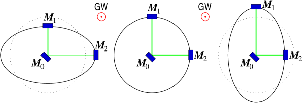
The physical meaning of the polarisation amplitudes in (12) is clarified by looking at the effect of an incoming wave on test particles. Consider e.g. two equal test masses whose center of mass is at the origin of $TT\/$ coordinates; let $\ell_{0}$ be their distance in the absence of GWs, and $(\theta,\varphi)$ the orientation (relative to the $TT\/$ axes) of the vector joining both masses. Making use of the geodesic deviation equation (2), with the Riemann tensor associated to (12), it can be seen that the GW only affects the transverse projection of the distance relative to the wave propagation direction (the $z\/$-axis); in fact, if $\ell(t)\equiv(\xi^{\mu}\,\xi_{\mu})^{1/2}$ is such distance then some simple algebra leads to the result

$$\ell(t)=\ell_{0}\,\left[1+\frac{1}{2}\,\left\{h_{+}(t)\,\cos 2\varphi+h_{\times}(t)\,\sin 2\varphi\right\}\,\sin^{2}\theta\right]\;.$$ (13)

Figure 1: The “$+$” and “$\times$” polarisation modes of a GW, according to GR theory. The dotted lines (circles) indicate the test particles’ position in the absence of GW signal. Each step in the graph corresponds to a quarter of the period of the driving GW, as labeled atop.

It is very important at this point to stress that the wavelength $\lambda$ of the incoming GW must be much larger than the distance $\ell(t)$ between the particles for (13) to hold, i.e.,

$$\ell(t)\ll\lambda\;,$$ (14)

and this is a condition which must be added to the already made assumption that $|h_{\mu\nu}|\ll 1$.

A graphical representation of the result (13) is displayed in figure 1: a number of test particles are evenly distributed around a circle perpendicular to the incoming GW, i.e., in the $xy\/$ plane. When a periodic signal comes in, the distances between those particles change following (13); note that the changes are modulated by the angular factors, i.e., according to the particles’ positions on the circle. The “$+$” mode is characterised by a vanishing wave amplitude $h_{\times}$, while in the “$\times$” mode $h_{+}$ vanishes.

2.2 Plane GWs according to metric theories of gravity

Although General Relativity has never been questioned so far by experiment, there are in fact alternative theories, e.g. Brans-Dicke theory bd61 , which are interesting for a number of reasons, for example cosmological reasons gazta . Generally, these theories make their own specific predictions about GWs, and they partly differ from those of GR – just discussed. The term metric theory indicates that the gravitational interaction affects the geometry of space-time, i.e., the metric tensor $g_{\mu\nu}$ is a fundamental ingredient – though other fields may also be necessary to complete the theoretical scheme. Obviously, General Relativity falls within this class of theories.

The appropriate scheme to assess the physics of such more general class of GWs was provided long ago el73 . The idea is to consider only plane gravitational waves, which should be an extremely good approximation for astrophysics, given our great distance even to the nearest conceivable GW source, and to characterise them by their Newman-Penrose scalars chan .

It appears that only six components of the Riemann tensor out of the usual 20 are independent in a plane GW; these are given by the four Newman-Penrose scalars

$$\mbox{{Y}}_{2}(v),\mbox{{Y}}_{3}(v),\mbox{{Y}}_{4}(v)\ \;{\rm y}\ \;\mbox{{F}}_{22}(v)\;,$$ (15)

of which $\mbox{{Y}}_{2}$ and $\mbox{{F}}_{22}$ are real, while $\mbox{{Y}}_{3}$ and $\mbox{{Y}}_{4}$ are complex functions of the null variable $v\/$ – see chan for all notation details. If a quasi-Lorentzian coordinate system is chosen such that GWs travel along the $z\/$-axis then $v=t-z$, and one can calculate the scalars (15) to obtain

$$\halign to=433.62pt{\@eqnsel\hskip\@centering$\displaystyle{#}$&\global\@eqcnt\@ne\hskip 2\arraycolsep\hfil${#}$\hfil&\global\@eqcnt\tw@\hskip 2\arraycolsep$\displaystyle{#}$\hfil&\llap{#}\cr\hfil\hskip 0.0pt plus 1000.0pt$\displaystyle{\mbox{{Y}}_{2}(t-z) &10.0pt\hfil${= &10.0pt$\displaystyle{-\mbox{\large$\frac{1}{6}$}\,R_{tztz}\;, {}&\hbox to0.0pt{\hss{\rm(0.16a)}\cr\penalty 100\vskip 3.0pt\vskip 0.0pt\cr\hfil\hskip 0.0pt plus 1000.0pt$\displaystyle{\mbox{{Y}}_{3}(t-z) &10.0pt\hfil${= &10.0pt$\displaystyle{-\mbox{\large$\frac{1}{2}$}\,(-R_{txtz}+{\rm i}R_{tytz})\;, {}&\hbox to0.0pt{\hss{\rm(0.16b)}\cr\penalty 100\vskip 3.0pt\vskip 0.0pt\cr\hfil\hskip 0.0pt plus 1000.0pt$\displaystyle{\mbox{{Y}}_{4}(t-z) &10.0pt\hfil${= &10.0pt$\displaystyle{-R_{txtx}+R_{tyty}+2{\rm i}R_{txty}\;, {}&\hbox to0.0pt{\hss{\rm(0.16c)}\cr\penalty 100\vskip 3.0pt\vskip 0.0pt\cr\hfil\hskip 0.0pt plus 1000.0pt$\displaystyle{\mbox{{F}}_{22}(t-z) &10.0pt\hfil${= &10.0pt$\displaystyle{-R_{txtx}-R_{tyty}\;. &\hbox to0.0pt{\hss{\rm(0.16d)}\cr}}}}}}}}}}}}}}}}}$$

General Relativity is characterised by $\mbox{{Y}}_{4}(t-z)$ being the only non-vanishing scalar, while in Brans-Dicke theory $\mbox{{F}}_{22}(t-z)$ also is different from zero – see el73 for full details.

It is relevant to remark at this stage that the only non-trivial components of the Riemann tensor of a plane GW are the so called “electric” components, $R_{titj}$, as we see in equations (2.2–d) above. These are, incidentally, also the only ones which appear in the geodesic deviation equation (2), since one may naturally choose $\dot{x}^{\mu}=(1;0,0,0)$ .

Figure 2: The six polarisation modes of a plane, metric GW. The dotted and solid lines correspond to distributions separated by a half period of the incoming wave, and it is assumed that the particles lie on a circle when no GW is acting. Note the indicators that the modes in the upper row are excited by a wave which arrives perpendicular to the particles’ plane, while those in the lower row correspond to GWs which are in the same plane as the particles. It must however be clarified that the mode $\mbox{{F}}_{22}$ has spherical symmetry, so it includes a combination of longitudinal and transverse excitations in like proportions.

This fact helps us make a graphical representation of all six possible polarisation states of a general metric GW in the same manner as in figure 1. The result is represented in figure 2 – whose source is reference will . The idea is to take a ring of test particles, let a GW pass by, and analyse the results of the displacements it causes in the distributions of those particles, just as done in section 2.2. Note that the first three modes are transverse, while the other three are longitudinal – see the caption to the figure. As already stressed, GR only gives rise to the two $\mbox{{Y}}_{4}$ modes.

3 Gravitational wave detection concepts

We are now ready to discuss the objectives and procedures to detect GWs: knowing their physical structure, one can design systems whose interaction with the GWs be sufficiently well understood and under control; suitable monitoring of the dynamics of such systems will be the source of information on whatever GW parameters may show up in a given observation experiment.

There are two major detection concepts: interferometric and acoustic detection. Historically, the latter came first through the pioneering work of J. Weber, but interferometric GW antennas are at present attracting the larger stake of the investment in this research field, both in hardware and in human commitment. This is because much hope has been deposited in their capabilities to reach sufficient sensitivity to measure GWs for the first time.

Interferometric detectors aim to measure phase shifts between light rays shone along two different (straight) lines, whose ends are defined by freely suspended test masses. This is done in a Michelson layout, using mirrors, beam splitters and photodiodes. Acoustic detectors are instead based on elastically linked test masses – rather than freely suspended – which resonantly respond to GW excitations.

These qualitative ideas can be made quantitatively precise, but the process is a non-trivial one and has important subtleties which must be properly understood for a thorough assessment of the detector workings and readout. The next sections are devoted to explain with some detail which are the theoretical principles governing the behaviour and response of both kinds of GW antennas.

4 Interferometric GW detectors

A rather naïve idea to measure the effect of an incoming GW is provided by the following argument – see also figure 3 for reference: let a GW having a “$+$” polarisation (assume GR for simplicity at this stage) come in perpendicular to the local horizontal at a given observatory; if three masses are laid down on the vertices of an ideally oriented isosceles right triangle then, as we saw (figure 1), the catets shrink and stretch with opposite phases. If a beam of laser light is now shone into the system, and a beam-splitter attached to mass $M_{0}$ and mirrors attached to $M_{1}$ and $M_{2}$, then one can think of measuring the distance changes between the masses by simple interferometry.

Figure 3: The “naïve” interferometric detector concept: a GW coming perpendicular to the sheet’s plane, “$+$” polarised relative to the $x\/$ and $y\/$ axes, causes the end masses $M_{1}$ and $M_{2}$ to oscillate in phase opposition relative to the central mass $M_{0}$. Light is shone into the system, and suitable beam splitters and mirrors are attached to the masses; length changes are then measured interferometrically, which directly lead to determine the GW amplitude.

This may look like a very reasonable proposal for a detector yet the following criticism readily suggests itself: gravitation is concerned with geometry, i.e., gravitational fields alter lengths and angles; therefore GWs will affect identically both distances between the masses of figure 3 and the wavelength of the light travelling between them – thus leading to a cancellation of the conjectured interferometric effect…

While the criticism is certainly correct, the conclusion is not. The reason is that it overlooks the fact that gravitation is concerned with the geometry of space-time – not just space. In the case of the above GW it so happens that, in $TT\/$ coordinates, the time dimension of space-time is not warped in the GW geometry – see the form of the metric tensor in equation (12) – while the transverse space dimensions are. Consequently an electromagnetic wave travelling in the $xy\/$ plane experiences wavelength changes depending on the propagation direction, but it does not experience frequency changes. The net result of this is that the phase of the electromagnetic wave differs from direction to direction of the $xy\/$ plane, and this makes a GW amenable to detection by interferometric principles.

Looked at in this way, the masses represented in figure 3 only play a passive role in the detector, in the sense that they simply make the interference between the two light beams possible by providing physical support for the mirrors and beam splitters. In other words, the physical principles underlying the working of an interferometric GW detector must have to do with the interaction between GWs and electromagnetic waves rather than with geodesic deviations of the masses.

Admittedly, this is not the most common point of view brian . It can however be made precise by the following considerations, which are studied in depth in references cqg and fara .

4.1 Test light beams in a GW-warped space-time

According to the above, it appears that we must address the question of how GW-induced fluctuations in the geometry of a background space-time affect the properties (amplitude and phase) of a plane electromagnetic wave – a light beam – which travels through such space-time. It will be sufficient to consider that the light beam is a test beam, i.e., its back action on the surrounding geometry is negligible.

Let then $A_{\mu}(\vec{x},t)$ be the vector potential which describes an electromagnetic wave travelling in vacuum; $A_{\mu}\/$ thus satisfies Maxwell’s equations

$$\raisebox{-1.2pt}{\Large$\Box$}A_{\mu}=0\;,$$ (17)

where $\Box$ stands for the generalised d’Alembert operator:

$$\raisebox{-1.2pt}{\Large$\Box$}\equiv g^{\rho\sigma}\,\nabla_{\rho}\nabla_{\sigma}\;.$$ (18)

We need only retain first order terms in $h_{\mu\nu}$ in the covariant derivatives, so that equation (17) reads

$$\raisebox{-1.2pt}{\Large$\Box$}A_{\mu}\simeq\eta^{\rho\sigma}\,(\partial_{\rho}\partial_{\sigma}A_{\mu}-2\Gamma_{\mu\sigma}^{\nu}\,\partial_{\rho}A_{\nu}-\Gamma_{\rho\sigma}^{\nu}\,\partial_{\nu}A_{\mu}-A_{\nu}\,\partial_{\rho}\Gamma_{\mu\sigma}^{\nu})=0\;,$$ (19)

To this equation, gauge conditions must be added. We shall conventionally adopt the usual Lorentz conditions, $\nabla_{\!\!\mu}A^{\mu}=0$, which, to lowest order in the gravitational perturbations, read

$$\nabla_{\!\mu}A^{\mu}\simeq-\partial_{t}A_{t}+\partial_{x}A_{x}+\partial_{y}A_{y}+\partial_{z}A_{z}-h^{\mu\nu}\,\partial_{\mu}A_{\nu}=0\;.$$ (20)

In addition to the weakness of the GW perturbation, it is also the case in actual practice that:

• The GW typical frequencies, $\omega$, are much smaller than the frequency of the light, $\Omega$: $\omega\ll\Omega$.

• The wavelength of the GW is much larger than the cross sectional dimensions of the light beam.

Wave front distortions and beam curvature are effects which can also be safely neglected in first order calculations fara . Finally, I shall make the simplifying assumption of perpendicular incidence, i.e., the incoming GW propagates in a direction orthogonal to the interferometer’s arms.

We shall thus consider one of the interferometer arms aligned with the $x\/$-direction, and the other with the $y\/$-direction, while the incoming GW will be assumed to approach the detector down the $z\/-axis$. The interaction GW-light beam will thus occur in the $z=0$ plane, hence the GW perturbations can be suitably described by a function of time alone, i.e.,

$$h_{\mu\nu}(\vec{x},t)\longrightarrow h_{\mu\nu}(\omega t)\;,$$ (21)

where $\omega$ is the frequency of the GW, which we can also safely assume to be plane-fronted, since its source will in all cases of interest be far removed from the observatory. In addition, for a beam running along the $x-axis$, the electromagnetic vector potential will only depend on the space variable $x\/$ and on time, i.e.,

$$A_{\mu}(\vec{x},t)\longrightarrow A_{\mu}(x,t)\;.$$ (22)

The following ansatz suggests itself for a solution to equations (19):

$$\halign to=433.62pt{\@eqnsel\hskip\@centering$\displaystyle{#}$&\global\@eqcnt\@ne\hskip 2\arraycolsep\hfil${#}$\hfil&\global\@eqcnt\tw@\hskip 2\arraycolsep$\displaystyle{#}$\hfil&\llap{#}\cr\hfil\hskip 0.0pt plus 1000.0pt$\displaystyle{A_{t}\,(t,x) &10.0pt\hfil${= &10.0pt$\displaystyle{\varepsilon_{0}(\omega t)\;, {}&\hbox to0.0pt{\hss{\rm(0.23a)}\cr\penalty 100\vskip 3.0pt\vskip 0.0pt\cr\hfil\hskip 0.0pt plus 1000.0pt$\displaystyle{A_{x}\,(t,x) &10.0pt\hfil${= &10.0pt$\displaystyle{\varepsilon_{1}(\omega t)\;, {}&\hbox to0.0pt{\hss{\rm(0.23b)}\cr\penalty 100\vskip 3.0pt\vskip 0.0pt\cr\hfil\hskip 0.0pt plus 1000.0pt$\displaystyle{A_{y}\,(t,x) &10.0pt\hfil${= &10.0pt$\displaystyle{a_{2}\;\exp[{\rm i}\Omega\,(t-x)]\, {\rm e}^{{\rm i}\,\phi_{2}(\omega t)}\;, {}&\hbox to0.0pt{\hss{\rm(0.23c)}\cr\penalty 100\vskip 3.0pt\vskip 0.0pt\cr\hfil\hskip 0.0pt plus 1000.0pt$\displaystyle{A_{z}\,(t,x) &10.0pt\hfil${= &10.0pt$\displaystyle{a_{3}\;\exp[{\rm i}\Omega\,(t-x)]\, {\rm e}^{{\rm i}\,\phi_{3}(\omega t)}\;, &\hbox to0.0pt{\hss{\rm(0.23d)}\cr}}}}}}}}}}}}}}}}}$$

where $\varepsilon_{0}(\omega t)$, $\varepsilon_{1}(\omega t)$, $\phi_{2}(\omega t)$ and $\phi_{3}(\omega t)$ are small quantities of order $h\/$, $a_{2}$ and $a_{3}$ are constants, and $\Omega$ is the frequency of the light. Clearly, these expressions reproduce the plane wave solutions to vacuum Maxwell’s equations in the limit of flat space-time, i.e., when $h_{\mu\nu}=0$.

Let us now take an incoming GW of the form

$$h_{\{+,\times\}}(t)=\tilde{H}_{\{+,\times\}}\,\mathrm{e}^{{\rm i}\omega t}\;,$$ (24)

and substitute it into (19) and (20), with the ansatz (4.1-d), neglecting higher order terms in the ratio $\omega/\Omega$. Then cqg , both $\phi_{2}$ and $\phi_{3}$ are seen to satisfy the approximate differential equation

$$\ddot{\phi}(t)+\frac{2{\rm i}\Omega}{\omega}\,\dot{\phi}(t)+\frac{{\rm i}\Omega^{2}}{\omega^{2}}\,h_{+}(t)=0\;.$$ (25)

The solution to this equation which is independent of the initial conditions is, to the stated level of accuracy,

$$\phi_{2}(t)\simeq\phi_{3}(t)\simeq\frac{\Omega}{2\omega}\,\tilde{H}_{+}\sin\omega t\;.$$ (26)

As shown in reference cqg , we need not worry about either $\varepsilon_{0}(\omega t)$ or $\varepsilon_{1}(\omega t)$ at this stage because the longitudinal component of the electric field (i.e., $E_{x}\/$) is an order of approximation smaller than the transverse components, which are given by

$$E_{y}=\partial_{t}A_{y}\ ,\qquad E_{z}=\partial_{t}A_{z}\;,$$ (27)

hence

$$\halign to=433.62pt{\@eqnsel\hskip\@centering$\displaystyle{#}$&\global\@eqcnt\@ne\hskip 2\arraycolsep\hfil${#}$\hfil&\global\@eqcnt\tw@\hskip 2\arraycolsep$\displaystyle{#}$\hfil&\llap{#}\cr\hfil\hskip 0.0pt plus 1000.0pt$\displaystyle{E_{y}(x,t) &10.0pt\hfil${\simeq&10.0pt$\displaystyle{{\rm i}\Omega\,a_{2}\,\exp\left[{\rm i}\Omega(t-x) + {\rm i}\,\frac{\Omega}{2\omega}\,\tilde{H}_{+}\sin\omega t\right]\;, {}&\hbox to0.0pt{\hss{\rm(0.28a)}\cr\penalty 100\vskip 3.0pt\vskip 4.30554pt\cr\hfil\hskip 0.0pt plus 1000.0pt$\displaystyle{E_{z}(x,t) &10.0pt\hfil${\simeq&10.0pt$\displaystyle{{\rm i}\Omega\,a_{3}\,\exp\left[{\rm i}\Omega(t-x) + {\rm i}\,\frac{\Omega}{2\omega}\,\tilde{H}_{+}\sin\omega t\right]\;. &\hbox to0.0pt{\hss{\rm(0.28b)}\cr}}}}}}}}}$$

These expressions beautifully show how the incoming GW causes a phase shift in an electromagnetic beam of light. Note that this phase shift is a periodic function of time, with the frequency of the GW. If we consider a real interferometer, such as very schematically shown in figure 3, and call $\tau\/$ the round trip time for the light to go from $M_{0}$ to $M_{2}$ and back, then the accumulated phase shift is, according to these formulas,

$$\delta_{x}\phi=2\times\frac{\Omega}{2\omega}\,\tilde{H}_{+}\sin\frac{\omega\tau}{2}\;,$$ (29)

since there is an obvious symmetry between light rays travelling to the right and to the left for a GW arriving perpendicularly to them.

The arguments leading to equations (4.1-b) can be very easily reproduced, mutatis mutandi, to obtain the phase shift experienced by a light ray travelling in the $y$, rather than the $x\/$ direction – everything in fact amounts to a simple interchange $\{x\longleftrightarrow y\}$ in the equations, which includes $\{h_{+}\longleftrightarrow-h_{+}\}$ as this is equivalent to $\{h_{xx}\longleftrightarrow h_{yy}\}$, see (12). The result is

$$\delta_{y}\phi=-2\times\frac{\Omega}{2\omega}\,\tilde{H}_{+}\sin\frac{\omega\tau}{2}\;.$$ (30)

In the actual interferometer, provided it has equal arm lengths, the two laser rays recombine in the beam splitter with a net phase difference

$$\delta\phi=\delta_{x}\phi-\delta_{y}\phi=\frac{2\Omega}{\omega}\,\tilde{H}_{+}\sin\frac{\omega\tau}{2}\;,$$ (31)

and this produces an interference signal, which is in principle measurable – if the instrumentation is sufficiently sensitive.

The reader may wonder how is it that the detector signal only depends on one of the GW amplitudes, $h_{+}$, but not on the other, $h_{\times}$. The reason is that we have made a very special assumption regarding the orientation of the GW’s polarisation axes relative to the light beam propagation directions. In a realistic case, even if perpendicular GW incidence happens, the detector’s arms will not be aligned with the GW’s natural axes, let alone the most likely case of oblique incidence. An important conclusion one should draw from this section is a conceptual one, that interferometric detectors are able to measure GW amplitudes and polarisations as a result of the interaction between the electromagnetic field of light rays and the background space-time geometry they travel across.

Beyond this, though, equation (31) has very relevant quantitative consequences, too. For example, as stressed in reference cqg , its range of validity is not limited to interferometer arms short compared to the GW wavelength. Therefore, according to the formula, a null effect (signal cancellation) happens if the round trip time $\tau$ equals the period of the GW, $2\pi/\omega$. Likewise, equation (31) also tells us that maximum detector signal occurs when $\tau=\pi/\omega$. All this happen to be true for arbitrary incidence and polarisation of the incoming GWs as well. For GW frequencies in the 1 kHz range, the best detector should thus have arm lengths in the range of 150 kilometers – and even longer for lower GW frequencies. No ground based GW antenna has ever been conceived of such dimensions yet there are intelligent ways to store the light in shorter arms for suitably tuned GW periods. I shall not go into details of these technical matters, see ron and brian for thorough information.

Figure 4: The acoustic detector concept: a GW coming perpendicular to the spring drives the two masses $M\/$ at its ends to oscillate at the GW’s frequency. Resonant amplification is obtained when the latter equals the spring’s characteristic frequency, $\Omega$.

5 Acoustic GW detectors

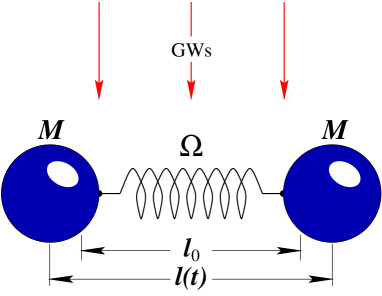
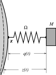
Acoustic GW detectors work based on a completely different concept – see figure 4: the idea is to set up test masses $M\/$ linked together by a spring of relaxed length $\ell_{0}$, so that GW tides drive their oscillations around the equilibrium position, with significant mechanical amplification at the spring’s characteristic frequency $\Omega$. The spring deformation

$$q(t)\equiv\ell(t)-\ell_{0}$$ (32)

thus obeys the following equation of motion:

$$\ddot{q}(t)+\Omega^{2}q(t)=\frac{1}{2}\,\ell_{0}\ddot{h}(t)\;,$$ (33)

where

$$h(t)=\left[h_{+}(t)\,\cos 2\varphi+h_{\times}(t)\,\sin 2\varphi\right]\,\sin^{2}\theta\;,$$ (34)

as follows from (13) – see also reference pizz for a complete discussion of this case.

This is the main idea, but in practice acoustic GW detectors are elastic solids rather than a single spring, i.e., they do not have a single characteristic frequency but a whole spectrum. The response of an elastic solid to a GW excitation is assessed by means of the classical theory of Elasticity, as described for example in ll70 . In such theory the deformations of the solid are given by the values of a vector field of displacements, $\vec{u}(\vec{x},t)$, which satisfies the evolution equations

$$\varrho\frac{\partial^{2}\vec{u}}{\partial t^{2}}-\mu\nabla^{2}\vec{u}-(\lambda+\mu)\,\nabla(\nabla{\bf\cdot}\vec{u})=\vec{f}(\vec{x},t)\;,$$ (35)

where $\varrho$ is the (undeformed) solid’s density, and $\lambda$ and $\mu\/$ are its Lamé coefficients, related to the Poisson ratio and Young modulus of the material the solid is made of ll70 . The function in the rhs of the equation is the density of external forces driving the motion of the system; in the present case, these are the tides generated by the sweeping GW, i.e.,

$$f_{i}(\vec{x},t)=\varrho\,R_{titj}(t)\,x_{j}\;,$$ (36)

where $R_{titj}(t)$ are components of the Riemann tensor evaluated at a fixed point of the solid, most expediently chosen at its center of mass. As already discussed in section 2.2, plane GWs have at most six degrees of freedom, adequately associated with the six electric components of the Riemann tensor, $R_{titj}(t)$. The six components are one monopole amplitude and five quadrupole amplitudes, and this important structure is made clear by the following expression of the density of GW tidal forces:

$$\vec{f}(\vec{x},t)=\vec{f}^{(0,0)}(\vec{x})\,g^{(0,0)}(t)\ +\ \sum_{m=-2}^{2}\,\vec{f}^{(2,m)}(\vec{x})\,g^{(2,m)}(t)\;,$$ (37)

which is entirely equivalent to (36) – see reference lobo –, and uses the common $(l,m)$ notation convention to indicate multipole terms. It is very important to stress at this stage that $\vec{f}^{(l,m)}(\vec{x})$ are pure form factors, simply depending on the fact that tides are monopole-quadrupole quantities, while all the relevant dynamic information carried by the GW is encoded in the time dependent coefficients $g^{(l,m)}(t)$. According to these considerations, we see that the ultimate objective of an acoustic GW antenna is to produce values of $g^{(l,m)}(t)$ – or indeed to extract from the device’s readout as much information as possible about those quantities.

Somewhat lengthy algebra permits to write down a formal solution to equations (36) and (37) in terms of an orthogonal series expansion lobo :

$$\vec{u}(\vec{x},t)=\sum_{N}\,\omega_{N}^{-1}\,\vec{u}_{N}(\vec{x})\,\left[\ \sum_{\stackrel{{\scriptstyle\scriptstyle l=0\ {\rm and}\ 2}}{{m=-l,...,l}}}\;f_{N}^{(l,m)}\,g_{N}^{(l,m)}(t)\,\right]\;,$$ (38)

where

$$\halign to=433.62pt{\@eqnsel\hskip\@centering$\displaystyle{#}$&\global\@eqcnt\@ne\hskip 2\arraycolsep\hfil${#}$\hfil&\global\@eqcnt\tw@\hskip 2\arraycolsep$\displaystyle{#}$\hfil&\llap{#}\cr\hfil\hskip 0.0pt plus 1000.0pt$\displaystyle{f_{N}^{(l,m)} &10.0pt\hfil${\equiv&10.0pt$\displaystyle{\frac{1}{M}\,\int_{\rm Solid}\vec{u}_{N}^{*}(\vec{x}) \cdot\vec{f}^{(l,m)}(\vec{x})\,\mathrm{d}^{3}x\;, {}&\hbox to0.0pt{\hss{\rm(0.39a)}\cr\penalty 100\vskip 3.0pt\vskip 4.30554pt\cr\hfil\hskip 0.0pt plus 1000.0pt$\displaystyle{g_{N}^{(l,m)}(t) &10.0pt\hfil${\equiv&10.0pt$\displaystyle{\int_{0}^{t}g^{(l,m)}(t')\,\sin\omega_{N}(t-t')\,\mathrm{d}t'\;, &\hbox to0.0pt{\hss{\rm(0.39b)}\cr}}}}}}}}}$$

with $M\/$ the whole solid’s mass; $omega_{N}\/$ is the (possibly degenerate) characteristic frequency of the elastic body, and $\vec{u}_{N}(\vec{x})$ the corresponding wavefunction, both determined by the solution to the eigenvalue problem

$$\mu\nabla^{2}\vec{u}_{N}+(\lambda+\mu)\,\nabla(\nabla\vec{\cdot}\vec{u}_{N})=-\omega_{N}^{2}\,\varrho\,\vec{u}_{N}\;,$$ (40)

with the boundary conditions that the surface of the solid be free of any tensions and/or tractions – see lobo for full details.

Historically, the first GW antennas were Weber’s elastic cylinders weber , but more recently, spherical detectors have been seriously considered for the next generation of GW antennas, as they show a number of important advantages over cylinders. I shall devote the next sections to a discussion of both types of systems, though clear priority will be given to spheres, due to their much richer capabilities and theoretical interest.

5.1 Cylinders

First thing to study the response of an elastic solid to an incoming GW is, as we have just seen, to determine its characteristic oscillation modes, i.e., its frequency spectrum $\omega_{N}$ and associated wavefunctions, $\vec{u}_{N}(\vec{x})$. In the case of a cylinder this is a formidable task; although its formal solution is known ric ; Ras , cylindrical antennas happen in practice tobe narrow and long expl ; naut , and so approximate solutions can be used instead which are much simpler to handle, and sufficiently good – see also wein .

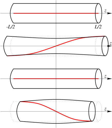
It appears that, in the long rod approximation, the most efficiently coupled modes are the longitudinal ones, and these have typical sinusoidal profiles, of the type

$$\delta z(z,t)\propto\sin\left(\frac{n\pi z}{L}\right)\,\sin\left(\frac{n\pi v_{s}t}{L}\right)\,\ ,\qquad n=1,2,3,\ldots$$ (41)

for a rod of length $L\/$ whose end faces are at $z=\pm L/2$, and in which the speed of sound is $v_{s}$. Figure 5 graphically shows the longitudinal deformations of the cylinder which correspond to (41), including transverse distortions which, though not reflected in the simplified equation (41), do happen in practice as a result of the Poisson ratio being different from zero ll70 . An important detail to keep in mind is that odd n modes have maximum displacements at the end faces, while even n modes have nodes there. In fact, the latter do not couple to GWs pizz . It is also interesting to stress that the center of the cylinder is always a node – this is relevant e.g. to suspension design issues naut .

Figure 5: The first longitudinal oscillation mode of a long cylinder. Note that it has a node at the center and maxima at the end faces. A whole period is represented, and transverse deformations are also shown.

A very useful concept to characterise the sensitivity of an acoustic antenna is its cross section for the absorption of GW energy. If an incoming GW flux density of $\Phi(\omega)$ watts per square metre and Hertz sweeps the cylinder and sets it to oscillate with energy $E(\omega)$ joules then the cross section is defined by the ratio

$$\sigma_{\rm abs}(\omega)=\frac{E(\omega)}{\Phi(\omega)}\;,$$ (42)

which is thus measured in m² Hz. Simple calculations show that, for optimal antenna orientation (perpendicular to the GW incidence direction) this quantity is given by pizz

$$\sigma_{\rm abs}(\omega_{n})=\frac{8}{\pi n^{2}}\;\frac{GMv_{s}^{2}}{c^{3}}\ ,\qquad n=1,3,5,\ldots\;,$$ (43)

where $M\/$ is the cylinder’s total mass.

It is interesting to get a flavour of the order of magnitude this quantity has: consider a cylinder of Al5056 (an aluminum alloy, for which $v_{s}\simeq 5400$ m/s), 3 metres long and 60 centimetres across, which has a mass of 2.3 tons; the above formula tells us that, for the first mode ($n=1$),

$$\sigma_{\rm abs}(\omega_{1})=4.3\times 10^{-21}\ {\rm cm}^{2}\,{\rm Hz}\;.$$ (44)

This is a very small number indeed, and gives an idea of how weak the coupling between GWs and matter is.

The weakness of the coupling gives an indication of how difficult it is to detect GWs. By the same token, though, GWs are very weakly damped as they travel through matter, which means they can produce information about otherwise invisible regions, such as the interior of a supernova, or even the big bang.

Equation (43) is only valid for perpendicular GW incidence. If incidence is instead oblique then a significant damping factor of $\sin^{4}\theta\/$ comes in, where $\theta\/$ is the angle between the GW direction and the cylinder’s axis pizz . This is a severe penalty, and it also happens in interferometric detectors not optimally oriented cqg ; st .

5.2 Solid spheres

The first initiatives to construct and operate GW detectors are due to J. Weber, who decided to use elastic cylinders. This philosophy and practice has survived him, and still today (February 2002) all GW detectors in continuous data taking regimes are actually Weber bars, though with significant sensitivity improvements bars derived, amongst other, from ultracryogenic and SQUID techniques.

About ten years after Weber began his research, R. Forward published an article fo71 where he pondered in a semi-quantitative way the potential virtues of a spherical, rather than cylindrical GW detector. Ashby and Dreitlein ad75 estimated how the whole Earth, as an auto-gravitating system, responds to GWs bathing it, and later Wagoner wp77 developed a theoretical model to study the response of an elastic sphere to GW excitations.

Interest in this new theoretical concept then waned to eventually re-emerge in the 1990s. The ALLEGRO detector group at Louisiana constructed a room temperature prototype antenna jm93 ; phd , which produced sound experimental evidence that it is actually possible to have a working system capable of making multimode measurements – I’ll come to this in detail shortly –, thus proving that a full-fledged spherical GW detector is within reach of current technological state of the art, as developed for Weber bars. It was apparently the fears to find unsurmountable difficulties in this problem which deterred further research on spherical GW antennas for years eug .

In this section I will give the main principles and results of the theory of the spherical GW detector, based on a formalism which has already been partly used in section 5, and for whose complete detail the reader is referred to lobo .

As we have seen, first thing we need is the eigenmodes and frequency spectrum of the spherical solid. This is a classical problem, long known in the literature, the solution to which I will briefly review here, with some added emphasis on the issues of our present concern.

The oscillation eigenmodes of a solid elastic body fall into two families: spheroidal and torsional modes lobo . Of these, only the former couple to GWs, while torsional modes do not couple at all bian . Spheroidal wavefunctions have the analytic form

$$\vec{u}_{nlm}(\vec{x})=A_{nl}(r)\,Y_{lm}(\vec{n})\,\vec{n}-B_{nl}(r)\,{\rm i}\vec{n}\!\times\!\vec{L}Y_{lm}(\vec{n})\;,$$ (45)

where $Y_{lm}$ are spherical harmonics ed60 , $\vec{n}=\vec{x}/R\/$ is the outward pointing normal, $\vec{L}$ is the ‘angular momentum operator’, $\vec{L}\equiv-{\rm i}\vec{x}\times\nabla$, $A_{nl}(r)$ and $B_{nl}(r)$ are somewhat complicated combinations of spherical Bessel functions lobo , and $\{nlm\}$ are ‘quantum numbers’ which label the modes. The frequency spectrum appears to be composed of ascending series of multipole harmonics, $\omega_{nl}$, i.e., for each multipole value $l\/$ there are an infinite number of frequency harmonics, ordered by increasing values of $n$. For example, there are monopole frequency harmonics $\omega_{10}$, $\omega_{20}$, $\omega_{30}$, etc.; then dipole frequencies $\omega_{11}$, $\omega_{21}$,…, then quadrupole harmonics $\omega_{12}$, $\omega_{22}$, and so on. Each of these frequencies is $(2l+1)$-fold degenerate, and this is a fundamental fact which makes of the sphere a theoretically ideal GW detector, as we shall shortly see.

If the above expressions are substituted into (5-b), then into (38), one easily obtains the sphere’s response function as

$$\vec{u}(\vec{x},t) = \sum_{n=1}^{\infty}\,\frac{a_{n0}}{\omega_{n0}}\,\vec{u}_{n00}(\vec{x})\,g_{n0}^{(0,0)}(t)$$ (46)

$$+ \sum_{n=1}^{\infty}\,\frac{a_{n2}}{\omega_{n2}}\,\left[\sum_{m=-2}^{2}\vec{u}_{n2m}(\vec{x})\,g_{n2}^{(2,m)}(t)\right]\;,$$ (47)

where

$$\halign to=433.62pt{\@eqnsel\hskip\@centering$\displaystyle{#}$&\global\@eqcnt\@ne\hskip 2\arraycolsep\hfil${#}$\hfil&\global\@eqcnt\tw@\hskip 2\arraycolsep$\displaystyle{#}$\hfil&\llap{#}\cr\hfil\hskip 0.0pt plus 1000.0pt$\displaystyle{a_{n0} &10.0pt\hfil${= &10.0pt$\displaystyle{-\frac{1}{M}\,\int_{0}^{R} A_{n0}(r)\,\rho\,r^{3}\,\mathrm{d}r\;, {}&\hbox to0.0pt{\hss{\rm(0.48a)}\cr\penalty 10000\vskip 3.0pt\vskip 10.00002pt\cr\hfil\hskip 0.0pt plus 1000.0pt$\displaystyle{a_{n2} &10.0pt\hfil${= &10.0pt$\displaystyle{-\frac{1}{M}\,\int_{0}^{R} \left[A_{n2}(r) + 3\,B_{n2}(r)\right]\,\rho\,r^{3}\,\mathrm{d}r\;, &\hbox to0.0pt{\hss{\rm(0.48b)}\cr}}}}}}}}}$$

and

$$g_{nl}^{(l,m)}(t)\equiv\int_{0}^{t}g^{(l,m)}(t^{\prime})\,\sin\omega_{nl}(t-t^{\prime})\,\mathrm{d}t^{\prime}\;.$$ (49)

Figure 6: The five quadrupole spheroidal oscillation modes of a solid elastic sphere, and the monopole mode. Note the latter (top left) is a spherically symmetric ‘breathing’ mode, while the rest have non-symmetric shapes. Because the eigenmodes (45) are actually complex (the spherical harmonics for $m\neq 0$ are complex) suitable combinations of them and their complex conjugates have been used to make plotting possible. These shapes are shared by all corresponding harmonics, i.e., quadrupole profiles for example are those shown no matter the harmonic number $n\/$ of their frequency $\omega_{n2}$: simply, they oscillate faster for higher $n\/$, but always keep the represented profile.

The series expansion (47) transparently shows that only monopole and quadrupole spherical modes can possibly be excited by an incoming GW. The monopole will of course not be excited at all if General Relativity is the true theory of gravitation. A spherical solid is thus seen to be the best possible shape for a GW detector. This is because of the optimality of the overlap coefficients $a_{nl}\/$ between the universal form factors $\vec{f}^{(l,m)}(\vec{x})$ and the sphere’s eigenmodes $\vec{u}_{nlm}(\vec{x})$, which comes about due to the clean multipole structure of the latter: only the $l\/$ = 0 and $l\/$ = 2 spheroidal modes couple to GWs, hence all the GW energy is deposited into them, and only them. Any other solid’s shape, e.g. a cylinder, has eigenmodes most of which have some amount of monopole/quadrupole projections in the form of the coefficients (5), and this means the incoming GW energy is distributed amongst many modes, thus making detection less efficient. We shall assess quantitatively the efficiency of the spherical detector in terms of cross section values below.

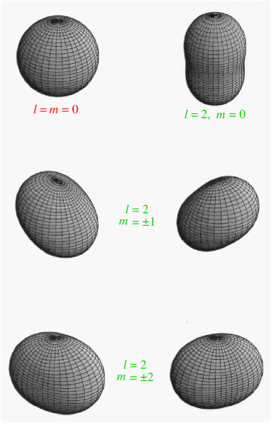
But, as just stated, quadrupole modes are degenerate. More specifically, they are 5-fold degenerate, each degenerate wavefunction corresponding to one of the five integer values $m\/$ can take between $-2$ and $+2$. Monopole modes are instead non-degenerate. Figure 6 shows the shapes of all these modes jao – see the caption to the figure for further details.

Degeneracy is a key concept for the multimode capabilities of the spherical detector. For, as explicitly shown by equation (47), monopole and quadrupole detector modes are driven by one and five GW amplitudes, respectively, i.e., $g^{(0,0)}(t)$ and $g^{(2,m)}(t)$. Therefore, if one could measure the amplitudes of these modes, i.e., the amplitudes of the deformations displayed in figure 6, then a complete deconvolution of the GW signal would be accomplished. This is a unique feature of the spherical antenna, which is not shared by any other GW detector: it enables the determination of all the GW amplitudes, not just a combination of them, no matter where the signal comes from. In section 5.3 below I shall give a more detailed review of how the multimode capability can be implemented in practice.

Cross sections

The general definition (42) applies in this case, too. Since cross section is a frequency dependent concept, and since quadrupole modes are degenerate, it is clear that energies deposited in each of the five degenerate modes of a given frequency harmonic must be added up to obtain $E(\omega_{n2})$ for that mode. Such energy must be calculated by means of volume integrals – to add up the energies of all differentials of mass throughout the solid –, the details of which I omit here. The final result turns out to be a remarkable one lobo : cross sections factorise in the form

$$\sigma_{\rm abs}(\omega_{nl})={\cal K}_{l}(\aleph)\,\frac{GMv_{t}^{2}}{c^{3}}\,(k_{nl}a_{nl})^{2}\qquad(l=0\mbox{\ or\ }2)\;,$$ (50)

where $GMv_{t}^{2}/c^{3}$ is a characteristic of the sphere’s material, and $(k_{nl}a_{nl})$ a dimensionless quantity associated with the $\{nl\}$-th frequency harmonic; finally, and this is the stronger theoretical point of this expression, ${\cal K}_{l}(\aleph)$ is a coefficient which is characteristic of the underlying theory of GWs, symbolically indicated with $\aleph$. For example, if the latter is General Relativity (GR) then

$$\aleph={\rm GR}\Rightarrow\left\{\begin{array}[]{l}{\cal K}_{0}(\aleph)=0\;,\\[6.99997pt] {\cal K}_{2}(\aleph)=\mbox{\Large$\frac{16\,\pi^{2}}{15}$}\;,\end{array}\right.$$ (51)

while if it is e.g. Brans-Dicke bd61 then these expressions get slightly more complicated bbc ; svino , etc.

Table 1: Compared characteristics and cross sections for a cylindrical and a spherical GW detector of like fundamental frequencies. Note that the cylinder is assumed to be optimally oriented, i.e., with its axis perpendicular to the GW incidence direction.

Cylinder	Sphere
$\nu_{1}$ = 910 Hz	$\left\{\begin{array}[]{l}\nu_{12}=910\ {\rm Hz}\\ \nu_{22}=1747\ {\rm Hz}\end{array}\right.$
$\left\{\begin{array}[]{l}L=3.0\ {\rm metres}\\ D=0.6\ {\rm metres}\end{array}\right.$	$2R\/$ = 3.1 metres
$M_{c}$ = 2.3 tons	$M_{s}$ = 42 tons
$\sigma_{1}=4.3$$\times$$10^{-21}$ cm2 Hz	$\left\{\begin{array}[]{l}\sigma_{12}=9.2\!\times\!10^{-20}\;{\rm cm}^{2}\ {\rm Hz}\\ \sigma_{22}=3.5\!\times\!10^{-20}\;{\rm cm}^{2}\ {\rm Hz}\end{array}\right.$
(Optimum orientation)	(Omnidirectional)

Sticking to GR, a few illustrative figures are in order. They are shown in table 1, where a material of aluminum Al5056 alloy has been chosen. It appears that a sphere having the same fundamental frequency ($\nu_{12}$) as a cylinder ($\nu_{1}$) is about 20 times more massive, and this results in a significant improvement in cross section, since it is proportional to the detector mass. A spherical detector is therefore almost one order of magnitude more sensitive than a cylinder in the same frequency band – obviously apart from the important fact that the sphere has isotropic sensitivity.

Figure 7: Cross section per unit mass of a cylinder and a sphere of like fundamental frequencies, in units of $Gv_{s}^{2}/c^{3}$. Note the (slightly) better figure (17 %) for the lowest mode in the sphere, as well as the appreciable value in the second harmonic of the latter, in sharp contrast with the null coupling of this mode in the cylinder. Third harmonics show a considerable reduction in sensitivity.

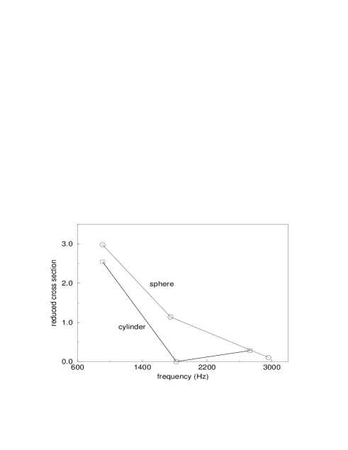
But there is more to this. Table 1 also refers to the sphere’s cross section in its second higher quadrupole harmonic frequency, $\nu_{22}$ – almost twice the value of the first, $\nu_{12}$. It is very interesting that cross section at this second frequency is only 2.61 times smaller than that at the first clo while, as stressed in section 2.1, it is zero for the second mode of the cylinder. Figure 7 shows a plot of the cross sections per unit mass of a cylinder and a sphere of like fundamental frequencies. It graphically displays the numbers given in the table, but also shows that, even per unit mass, the sphere is a better detector than a cylinder – its cross section ‘curve’ stays above the cylinder’s. In particular, the first quadrupole resonance turns out to have a cross section which is 1.17 times that of the cylinder (per unit mass, let me stress again) clo , i.e., $\sim$ 17 % better. This constitutes the quantitative assessment of the discussion in the paragraph immediately following equation (49).

5.3 The motion sensing problem

In order to determine the actual GW induced motions of an elastic solid a motion sensing system must be set up. In the case of currently operating cylinders this is done by what is technically known as resonant transducer paik . The idea of such device is to couple the large oscillating cylinder mass (a few tons) to a small resonator (less than 1 kg) whose characteristic frequency is accurately tuned to that of the cylinder. The joint dynamics of the resulting system $\{$cylinder + resonator$\}$ is a two-mode beat of nearby frequencies given by

$$\omega_{\pm}\simeq\omega_{0}\left(1\pm\frac{1}{2}\,\eta^{1/2}\right)\;,$$ (52)

where $\omega_{0}$ is the frequency of either oscillator when uncoupled to the other, and $\eta\equiv M_{\rm resonator}/M_{\rm cylinder}$. The key concept of this device is the resonant energy transfer, which flows back and forth between cylinder and sensor with the period of the beat, i.e., $2\pi(\eta\omega_{0})^{-1/2}$. This means that, because the sensor’s mass is very small compared to that of the cylinder, the amplitude of its oscillations is enhanced by a factor of $\eta^{-1/2}$ relative to those of the cylinder, whence a mechanical amplification factor is obtained before the sensor oscillations are converted to electrical signals, and further processed – see a more detailed account of these principles in amaldi2 .

The same principles can certainly be applied to make resonant motion sensors in a spherical antenna. In this case, however, a special bonus is there, associated to the degeneracy of the quadrupole frequencies: because all five quadrupole modes oscillate with the same frequency, it is possible to attach five (or more) identical resonators, tuned to a given quadrupole frequency, at suitable positions on the sphere surface, thus taking multiple samples of the sphere’s motion. This makes possible to retrieve the oscillation amplitudes of the five degenerate modes – figure 6 –, and thereby of the GW quadrupole amplitudes $g^{(l,m)}(t)$, since both are linearly related through equation (47).

A single spherical antenna can thus deconvolve completely the quadrupole GW signal, and do so with isotropic sky coverage. These characteristics are unique to the spherical detector, and they make it a theoretically superior system compared to either interferometers or Weber bars. In addition, a sphere can naturally measure the amplitude of the non-degenerate monopole mode, as it is conceptually simple to sense the amplitude of an isotropically breathing pattern.

Figure 8: Schematic diagramme of the coupling between a solid sphere and a resonator, modeled as a small mass linked to a spring attached to the sphere’s surface. The dashed-dotted arc line on the left indicates the position of the undeformed sphere’s surface, and the solid arc its actual position.

The conceptual idea of a resonant sensor is shown in figure 8, and the equations of motion for such a system are mnras

$$\halign to=433.62pt{\@eqnsel\hskip\@centering$\displaystyle{#}$&\global\@eqcnt\@ne\hskip 2\arraycolsep\hfil${#}$\hfil&\global\@eqcnt\tw@\hskip 2\arraycolsep$\displaystyle{#}$\hfil&\llap{#}\cr\hfil\hskip 0.0pt plus 1000.0pt$\displaystyle{\varrho\frac{\partial^{2} \vec{u}}{\partial t^{2}} &10.0pt\hfil${= &10.0pt$\displaystyle{\mu\nabla^{2} \vec{u} + (\lambda+\mu)\,\nabla(\nabla{\bf\cdot}\vec{u}) + {&\hbox to0.0pt{\hss\cr\penalty 100\vskip 3.0pt\vskip 0.0pt\cr}$\hfil& \sum_{b=1}^J M_b\Omega_b^2\,\left[z_b(t)-u_b(t)\right]\, \delta^{(3)}(\vec{x}-\vec{x}_b)\,\vec{n}_b + \vec{f}_{\rm GW}(\vec{x},t)\;, {} {\rm(0.53a)}\cr{\penalty 10000\vskip 3.0pt\vskip 6.99997pt} \ddot{z}_a(t) = -\Omega_a^2\, \left[z_a(t)-u_a(t)\right] + \xi_a^{\rm GW}(t)\ , \qquad a=1,\ldots,J\;, {\rm(0.53b)}\cr}$$ where $M_{a}$ and $\Omega_{a}$ are the mass and characteristic frequency of the $a$-th resonator, $\vec{f}_{\rm GW}(\vec{x},t)$ is the GW tide on the sphere -- see~{}(\ref{eq5.6}) --, and $\xi_{a}^{\rm GW}(t)$ is the GW induced tidal acceleration on the resonator itself, relative to the centre of the sphere; $\delta^{(3)}$ is the three dimensional Dirac density, i.e., point-like connections between sphere and sensors are assumed. The mathematical detail of the analysis of these equations is somewhat sophisticated. The interested reader will find complete information in~{}\cite[cite]{\@@bibref{Authors Phrase1YearPhrase2}{mnras}{\@@citephrase{(}}{\@@citephrase{)}}}; the rest of this section will be devoted to a brief discussion of the main conclusions of that analysis. \par First thing to stress is that equations~{}(\ref{eq5.20a}-b) cannot be solved analytically, they must instead be solved by a \emph{perturbative} procedure. The small perturbation parameters are the ratios \par\begin{equation}\eta_{a}\equiv\frac{M_{a}}{M}\ ,\qquad\eta_{a}\ll 1\ ,\qquad a=1,\ldots,J\;,\end{equation} where $M\/$ is the sphere's total mass. Actually, the analysis assumes that the resonators are all \emph{identical}, any deviations from this being eventually assessed by suitable methods~{}\cite[cite]{\@@bibref{Authors Phrase1YearPhrase2}{mnras,jm97}{\@@citephrase{(}}{\@@citephrase{)}}}. The fundamental result links the spring deformations to the the GW amplitudes $g^{(l,m)}(t)$ by the following formula, expressed in terms of \emph{Laplace transforms} -- noted with a caret (\,$\hat{}$\,): \par\begin{equation}\hat{q}_{a}(s)=\eta^{-1/2}\,\sum_{l,m}\,\hat{\Lambda}_{a}^{(lm)}(s;\Omega)\,\hat{g}^{(l,m)}(s)\ ,\qquad a=1,\ldots,J\;,\end{equation} where it is assumed that the resonators' frequency $\Omega$ is tuned to either a mono\-pole or a quadrupole harmonic of the sphere. The \emph{transfer functions} $\hat{\Lambda}_{a}^{(lm)}(s;\Omega)$ naturally depend on whether a monopole or a quadrupole mode is selected for resonator tuning; I will quote here only the quadrupole case, as it is the most interesting one -- see again full information in~{}\cite[cite]{\@@bibref{Authors Phrase1YearPhrase2}{mnras}{\@@citephrase{(}}{\@@citephrase{)}}}: \par\@@eqnarray\hat{\Lambda}_{a}^{(lm)}(s;\omega_{n2})&=&(-1)^{J}\,\sqrt{\frac{4\pi}{5}}\;a_{n2}\,\sum_{b=1}^{J}\,\left\{\sum_{\zeta_{c}\neq 0}\,\frac{1}{2}\left[\left(s^{2}+\omega_{c+}^{2}\right)^{-1}-\left(s^{2}+\omega_{c-}^{2}\right)^{-1}\right]\right.\\ &\times&\left.\frac{v_{a}^{(c)}v_{b}^{(c)*}}{\zeta_{c}}\right\}\,Y_{2m}(\vec{n}_{b})\,\delta_{l2}\;,\cr where $v_{a}^{(c)}$ is the $c\/$-th normalised eigenvector of the matrix $P_{2}(\vec{n}_{a}\!\cdot\vec{n}_{b})$, associated to its \emph{non-zero} eigenvalue $\zeta_{c}^{2}$, $P_{2}$ is a Legendre polynomial, and $\vec{n}_{a}$ is the position of the $a\/$-th resonator on the sphere's surface. Finally, \par\begin{equation}\omega_{a\pm}^{2}=\omega_{n2}^{2}\,\left(1\pm\sqrt{\frac{5}{4\pi}}\,\left|A_{n2}(R)\right|\,\zeta_{a}\,\eta^{1/2}\right)\ ,\qquad a=1,\ldots,J\;.\end{equation} \par Equations (\ref{eq5.22})--(\ref{eq5.24}) are the key to the GW signal deconvolution problem: they show that \emph{beats} occur around the tuned frequency ($\omega_{n2}$ in this case), and that the resonators oscillate with amplitudes enhanced by a factor $\eta^{-1/2}$, as indeed expected. Note that these beats have frequencies which depend on the resonators' positions $\vec{n}_{a}$, as shown by the presence of the~{}$\zeta_{a}$ coefficient in~{}(\ref{eq5.24}). \par\begin{figure}[b] \centering\includegraphics[width=256.0748pt]{fig9.eps} \@@toccaption{{\lx@tag[ ]{{9}}{The {\sl TIGA\/} and {\sl PHC\/} resonator distributions. In the former, \emph{six} sensors are attached to the pentagonal faces of a truncated icosahedron, while in the latter there are \emph{two} sets of \emph{five} quadrupole sensors, respectively tuned to the first quadrupole frequency (squares) and to the second (triangles); there is an 11-th sensor (star) which is tuned to a monopole frequency. The relevant common characteristic of these layouts is that they enable the definition of \emph{mode channels} --~{}see text for details. }}}\@@caption{{\lx@tag[: ]{{Figure 9}}{The {\sl TIGA\/} and {\sl PHC\/} resonator distributions. In the former, \emph{six} sensors are attached to the pentagonal faces of a truncated icosahedron, while in the latter there are \emph{two} sets of \emph{five} quadrupole sensors, respectively tuned to the first quadrupole frequency (squares) and to the second (triangles); there is an 11-th sensor (star) which is tuned to a monopole frequency. The relevant common characteristic of these layouts is that they enable the definition of \emph{mode channels} --~{}see text for details. }}}\@add@centering\end{figure} \par The deconvolution problem consists in inferring the GW amplitudes $\hat{g}^{(l,m)}(s)$ from the telescope's readouts $\hat{q}_{a}(s)$. Thus \emph{at least} 5 sensors must be attached to the sphere's surface if e.g.\ the 5 quadrupole amplitudes are looked for: once the corresponding five $\hat{q}_{a}(s)$ are \emph{measured} the system~{}(\ref{eq5.22}) is solved for $\hat{g}^{(2,m)}(s)$, that's it. \par Crucial at this point is to decide \emph{where} to implant the resonators, as such decision bears fundamentally on the simplicity, or even the possibility of solving the posed problem. There are two major proposals in the literature for this, and they are displayed in figure~{}\ref{fig9}. They permit the definition of so called \emph{mode channels}, which are linear combinations of the system readouts $\hat{q}_{a}(s)$ which are directly proportional to the GW amplitudes $\hat{g}^{(2,m)}(s)$. They happen to be of the form~{}\cite[cite]{\@@bibref{Authors Phrase1YearPhrase2}{mnras}{\@@citephrase{(}}{\@@citephrase{)}}} \par\begin{equation}\hat{y}^{(m)}(s)=\sum_{a=1}^{5\ {\rm or}\ 6}\,v_{a}^{(m)*}\hat{q}_{a}(s)\ ,\qquad m=-2,\ldots,2\;,\end{equation} both for {\sl TIGA\/} and {\sl PHC}. The actual result of these linear combinations is the following: \par\begin{equation}\hat{y}^{(m)}(s)=\eta^{-1/2}\,a_{n2}\,\frac{1}{2}\left[\left(s^{2}+\omega_{m+}^{2}\right)^{-1}-\left(s^{2}+\omega_{m-}^{2}\right)^{-1}\right]\,\hat{g}^{(2,m)}(s)\;,\end{equation} i.e., they are \emph{convolution products} of the signal and the system beats. \par This formula appears to be very powerful, as it shows that suitable sensor systems enable a \emph{single} spherical detector to fully deconvolve \emph{all} the GW amplitudes. One should however be careful about this conclusion, for the formula \emph{also} indicates that the relevant information \emph{can only be obtained at the resonance frequencies} $\omega_{m\pm}$ --~{}in an ideal, non-dissipative system. In a real system, resonant linewidths are never infinitely sharp, they have instead a certain breadth; this actually makes possible the observation across wider bandwidths, provided the amplifier noise can be kept sufficiently small --~{}I shall briefly come to this below in section~{}\ref{sec.6}. \par\par\par\@@numbered@section{subsection}{toc}{\bfit{Hollow} and \bfit{dual} spheres} \par The real merit of the just described spherical GW detector comes from its \emph{symmetry}. A \emph{hollow} sphere does of course share the symmetry properties of a solid sphere, and one might therefore expect it to be an interesting alternative, too. A detailed study of the performance of a hollow spherical GW detector can be found in~{}\cite[cite]{\@@bibref{Authors Phrase1YearPhrase2}{vega}{\@@citephrase{(}}{\@@citephrase{)}}}. The added bonus of a hollow sphere is that there is one more structural parameter one can adjust to enhance this or that property, and this is of course the \emph{thickness} of the spherical shell. It appears that cross sections at e.g.\ different quadrupole harmonics have characteristic behaviours when plotted as functions of thickness; also, one can decide to attach the motion sensors to the inner \emph{or} to the outer side of the shell, as their GW induced oscillations have different amplitudes. \par\begin{figure}[t] \centering\includegraphics[width=142.26378pt]{fig10.eps} \@@toccaption{{\lx@tag[ ]{{10}}{Conceptual scheme of the \emph{dual sphere}: the GW signal drives the facing surfaces between the nested spheres into oscillatory motions; when the signal frequency falls between the resonances of the spheres, oscillations happen with phase opposition, thereby enhancing the device's response. Motion sensing can be accomplished e.g.\ by non-resonant optical transducers. }}}\@@caption{{\lx@tag[: ]{{Figure 10}}{Conceptual scheme of the \emph{dual sphere}: the GW signal drives the facing surfaces between the nested spheres into oscillatory motions; when the signal frequency falls between the resonances of the spheres, oscillations happen with phase opposition, thereby enhancing the device's response. Motion sensing can be accomplished e.g.\ by non-resonant optical transducers. }}}\@add@centering\end{figure} \par To actually build and suspend a hollow sphere in the laboratory may be a difficult task from a technological point of view. Recently, though, a new concept spherical detector appeared in the literature~{}\cite[cite]{\@@bibref{Authors Phrase1YearPhrase2}{dual}{\@@citephrase{(}}{\@@citephrase{)}}}: this is called \emph{dual sphere}, and consists in a solid sphere nested inside a hollow one, concentric with it and with a narrow gap between them --~{}figure~{}\ref{fig10}. An incoming GW drives \emph{both} spheres into oscillation. Clearly, the inner solid sphere has a higher first (quadrupole) mode frequency than the outer hollow one, therefore an incoming GW with a frequency \emph{between} those two will drive the oscillations of the spheres with opposite phase, thus enhancing the signal by a rough factor of~{}2. \par The motion sensing in either hollow or dual spheres is conceptually analogous to that in the solid sphere, with the added flexibility that in the hollow piece one can choose to sense the displacements of either side of the shell. Actually, though, it appears that non-resonant detectors appear constitute a better choice in dual spheres, for this enables a significant bandwidth enlargement~{}\cite[cite]{\@@bibref{Authors Phrase1YearPhrase2}{dual}{\@@citephrase{(}}{\@@citephrase{)}}}. \par Let me briefly discuss now, for completeness, a few essentials of GW detector sensitivity. \par\par\par\@@numbered@section{section}{toc}{GW detector sensitivities} \par So far I have only discussed the \emph{theoretical} basis of the workings of GW detectors, whether interferometric or acoustic, yet have made no mention of the \emph{practical} difficulties of getting them actually working\ldots\par The extreme weakness of any expected GW signals arriving in the Earth~{}\cite[cite]{\@@bibref{Authors Phrase1YearPhrase2}{thorne}{\@@citephrase{(}}{\@@citephrase{)}}} is in fact a source of such truly difficult problems that it has prevented GW detectors from sighting a real signal in the last 40 years, since the times of J.~{}Weber. Local \emph{detector noise} has to date overwhelmed any signals possibly hitting the antennas, and therefore the technological challenge has been for years, and still is today, to reduce that noise to the level where it can be filtered out with a meaningful signal to noise ratio~{}\cite[cite]{\@@bibref{Authors Phrase1YearPhrase2}{klm93}{\@@citephrase{(}}{\@@citephrase{)}}}. \par During the last decade or so, a number of people in different countries worldwide have managed to get important GW detection research projects funded which constitute a major step forward in detector technology. Their goal is to improve the sensitivity to the point where a significant \emph{event rate} becomes available to the GW astronomer. We thus find such laboratories as {\sl VIRGO\/} (a French-Italian collaboration), {\sl LIGO\/} (USA alone), or {\sl LISA\/} (a space mission, jointly funded by {\sl NASA\/} and {\sl ESA}, the European Space Agency). In addition to those, somewhat smaller experiments are {\sl GEO-600\/} (a German-British venture) and {\sl TAMA\/} (the Japanese project, currently making strong progress in both and stability). \par So much for \emph{interferometric} antennas. But endeavours have not declined in the \emph{acoustic detector} arena, either. In fact, the five acoustic detectors of the Weber type ({\sl NAUTILUS, EXPLORER, AURIGA, ALLEGRO and NIOBE\/}) constitute the \emph{only working systems} in the world today. Unfortunately, though, they are only sensitive to catastrophic events happening in our galaxy, with a far too low occurrence rate. These detector systems are periodically upgraded, and their sensitivity has gone up a few orders of magnitude since their origins. As already stressed in section~{}\ref{sec.1}, new generation \emph{spherical} GW detectors are being programmed in Brazil, Holland and Italy, and these should suddenly improve over bars by at least one more order of magnitude. \par\begin{figure}[b] \centering\includegraphics[width=284.52756pt]{fig11.eps} \@@toccaption{{\lx@tag[ ]{{11}}{Spectral strain sensitivities of various future generation GW detectors, including the ``dual sphere''. }}}\@@caption{{\lx@tag[: ]{{Figure 11}}{Spectral strain sensitivities of various future generation GW detectors, including the ``dual sphere''. }}}\@add@centering\end{figure} \par Figure~{}\ref{fig.11} contains a recent plot of GW sensitivity of various earth based detectors, therefore in the frequency range near 1\,kHz. On the other hand, {\sl LISA\/} will be sensitive at frequencies far away from the range plotted in figure~{}\ref{fig.11} --~{}see {\sl LISA}'s web site at {\tt http://sci.esa.int/home/lisa} and figure~{}\ref{fig.12} below. What we see in ordinates in plots like the one in figure~{}\ref{fig.11}, which are standard in GW science, is a \emph{spectral density} --~{}or, rather, its \emph{square root}. It is to be understood as follows. \par\emph{Noise} of whatever origin causes any detector to generate random outputs --~{}\emph{stochastic} time series, as this is technically known. This noise competes with any GW signals which may be present in the antenna readout, obscuring their detection. Noise of course does not come from the sky, it rather gets added to the GW signal at almost all the different stages of the detection process. For example, the GW induced oscillations of a given mass compete with thermal oscillations of that mass and its suspension systems; then there is noise in the conversion from mechanical or optical GW signals to electrical signals; then there is noise introduced by the electronics in the amplifiers of the latter; and so forth\ldots\par In the end, the detector output is a certain physical magnitude (e.g.\ a voltage) which consists of a number of various superimposed sources of noise plus, possibly, a GW signal \emph{converted} to volts by the detector hardware. One infers the value of the \emph{actual} dimensionless GW amplitude $h(t)$, say, from the output voltage if one knows the precise physics of the transduction process --~{}and this is obviously the case in any useful instrument. \par Conversely, it is also possible to \emph{back-convert} all the sources of noise voltage picked up across the various detector stages to an equivalent dimensionless ``GW noise'', which gets directly added to real GW signals, and travels through an ideally noiseless detector. This artifact is expedient because, for a fixed antenna, it enables a quick assessment of the detectability of a given GW signal, normally calculated by methods of gravitation theory, by direct comparison with suitably constructed detector characteristic curves -- such as those in figure~{}\ref{fig.11}. \par Let us then call $x(t)$ any one of the detector's readout channels, \emph{back-con\-verted} to a GW amplitude by the above described procedure. We split this up into a GW signal proper $h(t)$ plus a noise term $n(t)$: \par\begin{equation}x(t)=h(t)+n(t)\;.\end{equation} \par For stationary Gaussian noise, the statistical properties of $n(t)$ are encoded in its \emph{spectral density} function, $S_{h}(\omega)$, which is the Fourier transform of the \emph{autocorrelation function} \par\begin{equation}R(\tau)\equiv\langle x(t)\,x(t+\tau)\rangle\ ,\qquad S_{h}(\omega)\equiv\int_{-\infty}^{\infty}\,R(\tau)\,\mathrm{e}^{{\rm i}\omega\tau}\,\mathrm{d}\tau\;,\end{equation} where $\langle-\rangle$ stands for \emph{ensemble average}~{}\cite[cite]{\@@bibref{Authors Phrase1YearPhrase2}{kay}{\@@citephrase{(}}{\@@citephrase{)}}}. It can be shown~{}\cite[cite]{\@@bibref{Authors Phrase1YearPhrase2}{klm93}{\@@citephrase{(}}{\@@citephrase{)}}} that the \emph{optimum filter} to extract the signal $h(t)$ from the system readout $x(t)$ is the so called \emph{matched filter}, whose transfer function is the signal's Fourier transform $\tilde{h}(\omega)$ divided by the spectral density $S_{h}(\omega)$, and the \emph{detection threshold} can be set from the integrated signal to noise ratio: \par\begin{equation}SNR=\int_{-\infty}^{\infty}\,\frac{|\tilde{h}(\omega)|^{2}}{S_{h}(\omega)}\,\frac{\mathrm{d}\omega}{2\pi}\;.\end{equation} \par The GW signal $h(t)$ is a dimensionless quantity, as it measures a perturbation of the Minkowski metric, see equation~{}(\ref{eq2.2}). Therefore the spectral density $S_{h}(\omega)$ has dimensions of time, or inverse frequency, Hz$^{-1}$, according to the definitions~{}(\ref{eq5.28}). Now, signal to noise ratio as defined by the integral~{}(\ref{eq5.29}) is made up of the contributions of the ratio between the signal power $|\tilde{h}(\omega)|^{2}$ to the noise power $S_{h}(\omega)$ at all frequencies; the idea of the graphical representation in figure~{}\ref{fig.11} is thus to show which is the level of noise at different frequencies by means of an rms quantity, such as is the square root of the noise spectral density. The appropriate units for this representation are accordingly Hz$^{-1/2}$, as indicated. \par\begin{figure}[t] \centering\includegraphics[width=341.43306pt]{fig12.eps} \@@toccaption{{\lx@tag[ ]{{12}}{Root mean square noise spectral densities, referred to GW amplitudes, for some of the upcoming interferometric GW detectors, together with the spectral intensities of various signals. The latter are estimated by numerical calculation, while the noise is modeled on the basis of its origin and instrumental characteristics. See~{}\cite[cite]{\@@bibref{Authors Phrase1YearPhrase2}{bfs}{\@@citephrase{(}}{\@@citephrase{)}}}. }}}\@@caption{{\lx@tag[: ]{{Figure 12}}{Root mean square noise spectral densities, referred to GW amplitudes, for some of the upcoming interferometric GW detectors, together with the spectral intensities of various signals. The latter are estimated by numerical calculation, while the noise is modeled on the basis of its origin and instrumental characteristics. See~{}\cite[cite]{\@@bibref{Authors Phrase1YearPhrase2}{bfs}{\@@citephrase{(}}{\@@citephrase{)}}}. }}}\@add@centering\end{figure} \par Different interesting sources of GWs are being considered by other authors in this volume, so I will not go into such matters here. It is nevertheless instructive to present an example graph of a few signals on top of various detectors' sensitivity curves in order to get a picture of the actual possibilities of each instrument, and also to grasp what are the spectral orders of magnitude of different GW signals. One such plot is presented in figure~{}\ref{fig.12}. This is, let me insist, the standard way to assess the detectability of the different GW sources. \par\par\par\@@numbered@section{section}{toc}{Concluding remarks} \par This article is a brief review on the nature of the interactions of GWs with \emph{test} particles and \emph{test} electromagnetic fields, as they specifically happen in currently conceived detection devices. While the fundamental principles are not new in themselves, their application in actual systems is still in many cases subject of research, as we have seen. A thorough understanding of these matters is absolutely essential for an adequate interpretation of the antenna readouts, the more so if one considers the extreme \emph{weakness} of any signals reaching us from even the most intense sources. \par I have omitted any detailed discussion of the practical problems faced by real detector building. This is a major research field in itself, of an intrinsically sophisticated and multidisciplinary nature -- involving such fundamental issues as quantum measurement limits and techniques, or Quantum Optics~{}\cite[cite]{\@@bibref{Authors Phrase1YearPhrase2}{brag}{\@@citephrase{(}}{\@@citephrase{)}}}. But it is of course not directly related to Astrophysics or Relativity\ldots\ I have however considered appropriate to summarily brief the interested reader on how detector sensitivities are defined, and on which are the detection thresholds in current state of the art GW detectors: this is a key issue for an astrophysicist/relativist wishing to assess the detectability of a given GW signal, whether by existing instruments or future planned. \par GW detection endeavours have been the subject of intensive research during the last 4 decades, though the ultimate goal of sighting GW events has still not been accomplished. While this may look like a major failure, one may not forget that detector sensitivities have gone up by a remarkable \emph{six orders of magnitude} (in energy, three in GW amplitude) since the very first telescopes constructed by J.~{}Weber. Also, a look at the trend in this development indicates that we are getting closer to the obejctive. \par Prospects look now better than ever yet the real challenge is still there\ldots\par\par\thebibliography\addcontentsline{toc}{section}{References} \@@lbibitem{ein18}\NAT@@wrout{1}{}{}{}{(1)}{ein18}\lx@bibnewblock A.\ Einstein: Sitz.\ Ber.\ K\"{o}n.\ Preus.\ Ak.\ Wiss., p.\ 688 (1916), and p.\ 154 (1918) \par\@@lbibitem{mtw}\NAT@@wrout{2}{}{}{}{(2)}{mtw}\lx@bibnewblock C.W.\ Misner, K.S.\ Thorne, J.A.\ Wheeler: \emph{Gravitation} (Freeman, San Francisco~{}1973) \par\@@lbibitem{will}\NAT@@wrout{3}{}{}{}{(3)}{will}\lx@bibnewblock C.M.\ Will: \emph{Theory and experiment in Gravitational Physics} (Cambridge University Press, Cambridge 1993) \par\@@lbibitem{weber}\NAT@@wrout{4}{}{}{}{(4)}{weber}\lx@bibnewblock J.\ Weber: Phys.\ Rev.\ Lett.\ {\bf 22}, 1320 (1969); {\bf 24}, 276 (1970); {\bf 25}, 180 (1970) \par\@@lbibitem{jweb2}\NAT@@wrout{5}{}{}{}{(5)}{jweb2}\lx@bibnewblock J.\ Weber: `Supernova 1987\,A Rome and Maryland GW radiation antenna observations'. In: \emph{Gravitational wave experiments}, Proceedings of the 1st Edoardo Amaldi Conference, ed.\ by E.\ Coccia, G.\ Pizzella, F.\ Ronga (World Scientific, Singapore 1995), p.\ 416 \par\@@lbibitem{gh71}\NAT@@wrout{6}{}{}{}{(6)}{gh71}\lx@bibnewblock G.W.\ Gibbons, S.W.\ Hawking: Phys.\ Rev.\ D {\bf 4}, 2191 (1971) \par\@@lbibitem{weiss}\NAT@@wrout{7}{}{}{}{(7)}{weiss}\lx@bibnewblock R.\ Weiss: Quarterly Progress Report, Research Laboratory of Electronics {\bf 105}, 54 (MIT 1972) \par\@@lbibitem{ron}\NAT@@wrout{8}{}{}{}{(8)}{ron}\lx@bibnewblock R.\ Drever: `Interferometric detectors for gravitational radiation'. In: \emph{Gravitational radiation}, ed.\ by N.\ Deruelle and T.\ Piran (North Holland, Amsterdam 1983), p.~{}321 \par\@@lbibitem{igec}\NAT@@wrout{9}{}{}{}{(9)}{igec}\lx@bibnewblock G.A.\ Prodi et al.: Int.\ J.\ Mod.\ Phys.\ {\bf D9}, 237 (2000) \par\@@lbibitem{msch}\NAT@@wrout{10}{}{}{}{(10)}{msch}\lx@bibnewblock O.D.\ Aguiar \emph{et al.}: `The first phase of the Brazilian Graviton project'. In: \emph{Gravitational waves}, Proceedings of the 3rd Edoardo Amaldi Conference, ed.\ by S.\ Meshkov (World Scientific, Singapore 2000), p.\ 413 \par\@@lbibitem{mgrail}\NAT@@wrout{11}{}{}{}{(11)}{mgrail}\lx@bibnewblock G.\ Frossati: `{\sl MINIGRAIL}, a sensitive spherical gravitational wave antenna for frequencies around 3.6 kHz', Projectruimte Normale Programma FWO (Leiden~{}2000) \par\@@lbibitem{sfera}\NAT@@wrout{12}{}{}{}{(12)}{sfera}\lx@bibnewblock P.\ Astone \emph{et al.}: `{\sl SFERA\/}: Proposal for a spherical GW detector' (Roma 1997) \par\@@lbibitem{ht75}\NAT@@wrout{13}{}{}{}{(13)}{ht75}\lx@bibnewblock R.A.\ Hulse, J.H.\ Taylor: Astrophys.\ Jour.\ {\bf 195}, L51 (1975) \par\par\@@lbibitem{tay94}\NAT@@wrout{14}{}{}{}{(14)}{tay94}\lx@bibnewblock J.H.\ Taylor: Rev.\ Mod.\ Phys.\ {\bf 66}, 711 (1994) \par\par\par\@@lbibitem{wein}\NAT@@wrout{15}{}{}{}{(15)}{wein}\lx@bibnewblock S.\ Weinberg: \emph{Gravitation and Cosmology\/} (Wiley \& Sons, New York 1972) \par\@@lbibitem{grif}\NAT@@wrout{16}{}{}{}{(16)}{grif}\lx@bibnewblock J.B.\ Griffiths: \emph{Colliding plane waves in General Relativity} (Clarendon Press, Oxford 1991) \par\@@lbibitem{bd61}\NAT@@wrout{17}{}{}{}{(17)}{bd61}\lx@bibnewblock C.\ Brans, R.H.\ Dicke: Phys.\ Rev.\ {\bf 124}, 925 (1961) \par\@@lbibitem{gazta}\NAT@@wrout{18}{}{}{}{(18)}{gazta}\lx@bibnewblock E.\ Gazta\~{n}aga, J.A.\ Lobo: Astroph.\ Jour.\ {\bf 548}, 47 (2001) \par\@@lbibitem{el73}\NAT@@wrout{19}{}{}{}{(19)}{el73}\lx@bibnewblock D.M.\ Eardley, D.L.\ Lee, A.P.\ Lightman: Phys.\ Rev.\ D {\bf 8}, 3308 (1973) \par\@@lbibitem{chan}\NAT@@wrout{20}{}{}{}{(20)}{chan}\lx@bibnewblock S.\ Chandrasekhar: \emph{The mathematical theory of Black Holes} (Pergamon Press, Oxford 1983) \par\@@lbibitem{brian}\NAT@@wrout{21}{}{}{}{(21)}{brian}\lx@bibnewblock B.J.\ Meers: Phys.\ Rev.\ D {\bf 38}, 2317 (1988) \par\@@lbibitem{cqg}\NAT@@wrout{22}{}{}{}{(22)}{cqg}\lx@bibnewblock J.A.\ Lobo: Class.\ Quan.\ Grav.\ {\bf 9}, 1385 (1992) \par\@@lbibitem{fara}\NAT@@wrout{23}{}{}{}{(23)}{fara}\lx@bibnewblock F.I.\ Cooperstock, V.\ Faraoni: Class.\ Quan.\ Grav.\ {\bf 10}, 1189 (1993) \par\@@lbibitem{pizz}\NAT@@wrout{24}{}{}{}{(24)}{pizz}\lx@bibnewblock G.\ Pizzella: \emph{Fisica Sperimentale del Campo Gravitazionale} (Nuova Italia Scientifica, Roma 1993) \par\@@lbibitem{ll70}\NAT@@wrout{25}{}{}{}{(25)}{ll70}\lx@bibnewblock L.D.\ Landau, E.M.\ Lifshitz: {\it Theory of Elasticity} (Pergamon Press, Oxford 1970) \par\@@lbibitem{lobo}\NAT@@wrout{26}{}{}{}{(26)}{lobo}\lx@bibnewblock J.A.\ Lobo: Phys.\ Rev.\ D {\bf 52}, 591 (1995) \par\@@lbibitem{ric}\NAT@@wrout{27}{}{}{}{(27)}{ric}\lx@bibnewblock R.G.\ Hier, S.N.\ Rasband: Astroph.\ Jour.\ {\bf 195}, 507 (1975). \par\@@lbibitem{Ras}\NAT@@wrout{28}{}{}{}{(28)}{Ras}\lx@bibnewblock S.N.\ Rasband: Jour.\ Acous.\ Soc.\ Am.\ {\bf 57}, 899 (1975) \par\@@lbibitem{expl}\NAT@@wrout{29}{}{}{}{(29)}{expl}\lx@bibnewblock P.\ Astone {\it et al.}: Phys.\ Rev.\ D {\bf 47}, 362 (1993) \par\@@lbibitem{naut}\NAT@@wrout{30}{}{}{}{(30)}{naut}\lx@bibnewblock P.\ Astone {\it et al.}: Astropart.\ Phys.\ {\bf 7}, 231 (1997) \par\@@lbibitem{st}\NAT@@wrout{31}{}{}{}{(31)}{st}\lx@bibnewblock S.V.\ Dhurandhar, M.\ Tinto: Mon.\ Not.\ Roy.\ Astr.\ Soc.\ {\bf 234}, 663 (1988), and {\bf 236}, 621 (1989) \par\@@lbibitem{bars}\NAT@@wrout{32}{}{}{}{(32)}{bars}\lx@bibnewblock Z.A.\ Allen {\it et al.}: Phys.\ Rev.\ Lett.\ {\bf 85}, 5046 (2000) \par\@@lbibitem{fo71}\NAT@@wrout{33}{}{}{}{(33)}{fo71}\lx@bibnewblock R.\ Forward: Gen.\ Rel.\ Grav.\ {\bf 2}, 149 (1971) \par\@@lbibitem{ad75}\NAT@@wrout{34}{}{}{}{(34)}{ad75}\lx@bibnewblock N.\ Ashby, J.\ Dreitlein: Phys.\ Rev.\ {\bf D12}, 336 (1975). \par\@@lbibitem{wp77}\NAT@@wrout{35}{}{}{}{(35)}{wp77}\lx@bibnewblock R.V.\ Wagoner, H.J.\ Paik: `Multimode detection of gravitational waves by a sphere'. In: \emph{Experimental Gravitation}, Proceedings of the Pavia International Symposium, Accad.\ Naz.\ dei Lincei (Roma 1977) \par\@@lbibitem{jm93}\NAT@@wrout{36}{}{}{}{(36)}{jm93}\lx@bibnewblock W.W.\ Johnson, S.M.\ Merkowitz: Phys.\ Rev.\ Lett.\ {\bf 70}, 2367 (1993) \par\@@lbibitem{phd}\NAT@@wrout{37}{}{}{}{(37)}{phd}\lx@bibnewblock S.\ M.\ Merkowitz: Truncated Icosahedral Gravitational Wave Antenna. PhD Thesis Memoir, Louisiana State University (Baton Rouge 1995) \par\@@lbibitem{eug}\NAT@@wrout{38}{}{}{}{(38)}{eug}\lx@bibnewblock E.\ Coccia: private communication \par\@@lbibitem{bian}\NAT@@wrout{39}{}{}{}{(39)}{bian}\lx@bibnewblock M.\ Bianchi, E.\ Coccia, C.N.\ Colacino, V.\ Fafone, F.\ Fucito: Class.\ Quan.\ Grav.\ {\bf 13}, 2865 (1996) \par\@@lbibitem{ed60}\NAT@@wrout{40}{}{}{}{(40)}{ed60}\lx@bibnewblock A.R.\ Edmonds: \emph{Angular Momentum in Quantum Mechanics} (Princeton University Press, Princeton 1960) \par\@@lbibitem{jao}\NAT@@wrout{41}{}{}{}{(41)}{jao}\lx@bibnewblock J.A.\ Ortega: Spherical gravitational wave detectors. PhD Thesis Memoir, University of Barcelona (Barcelona 1997) \par\@@lbibitem{bbc}\NAT@@wrout{42}{}{}{}{(42)}{bbc}\lx@bibnewblock M.\ Bianchi, M.\ Brunetti, E.\ Coccia, F.\ Fucito, J.A.\ Lobo: Phys.\ Rev.\ D {\bf 57}, 4525~{}(1998) \par\@@lbibitem{svino}\NAT@@wrout{43}{}{}{}{(43)}{svino}\lx@bibnewblock E.\ Coccia, F.\ Fucito, J.A.\ Lobo, M.\ Salvino: Phys.\ Rev.\ D {\bf 62}, 044019-1 (2000) \par\@@lbibitem{clo}\NAT@@wrout{44}{}{}{}{(44)}{clo}\lx@bibnewblock E.\ Coccia, J.A.\ Lobo, J.A.\ Ortega: Phys.\ Rev.\ D {\bf 52}, 3735 (1995) \par\@@lbibitem{paik}\NAT@@wrout{45}{}{}{}{(45)}{paik}\lx@bibnewblock H.J.\ Paik: `Electromechanical transducers and bandwidth of resonant mass GW detectors'. In: \emph{Gravitational wave experiments}, Proceedings of the 1st Edoardo Amaldi Conference, ed.\ by E.\ Coccia, G.\ Pizzella, F.\ Ronga (World Scientific, Singapore 1995), p.\ 201 \par\@@lbibitem{amaldi2}\NAT@@wrout{46}{}{}{}{(46)}{amaldi2}\lx@bibnewblock J.A.\ Lobo: `Spherical gravitational wave detectors and geometry'. In: \emph{Gravitational waves}, Proceedings of the 2nd Edoardo Amaldi Conference, ed.\ by E.\ Coccia, G.\ Pizzella, G.\ Veneziano (World Scientific, Singapore 1998), p.\ 168 \par\@@lbibitem{mnras}\NAT@@wrout{47}{}{}{}{(47)}{mnras}\lx@bibnewblock J.A.\ Lobo: Mon.\ Not.\ Roy.\ Astr.\ Soc.\ {\bf 316}, 173 (2000). See also {\tt gr-qc/0006055} \par\@@lbibitem{jm97}\NAT@@wrout{48}{}{}{}{(48)}{jm97}\lx@bibnewblock S.M.\ Merkowitz, W.W.\ Johnson: Phys.\ Rev.\ D {\bf 56}, 7513 (1997) \par\@@lbibitem{vega}\NAT@@wrout{49}{}{}{}{(49)}{vega}\lx@bibnewblock E.\ Coccia, V.\ Fafone, G.\ Frossati, J.A.\ Lobo, J.A.\ Ortega: Phys.\ Rev.\ D {\bf 57}, 2051~{}(1998) \par\@@lbibitem{dual}\NAT@@wrout{50}{}{}{}{(50)}{dual}\lx@bibnewblock M.\ Cerdonio, L.\ Conti, J.A.\ Lobo, A.\ Ortolan, L.\ Taffarello, J.P.\ Zendri: Phys.\ Rev.\ Lett.\ {\bf 87}, 031101~{}(2001) \par\@@lbibitem{symon}\NAT@@wrout{51}{}{}{}{(51)}{symon}\lx@bibnewblock K.R.\ Symon: \emph{Mechanics}, 2nd edition, chapter 2 (Addison-Wesley, Reading 1960) \par\@@lbibitem{thorne}\NAT@@wrout{52}{}{}{}{(52)}{thorne}\lx@bibnewblock K.S.\ Thorne: `Gravitational radiation'. In: \emph{300 Years of Gravitation}, ed.\ by S.W.\ Hawking and W.\ Israel (Cambridge University Press, Cambridge 1988), p.\ 330. See also more recent reviews by K.S.\ Thorne, e.g.\ {\tt gr-qc/9704042}, or visit the website \verb=http://fermi.phys.ualberta.ca/~ccgrra/thorne/index.html= \par\@@lbibitem{klm93}\NAT@@wrout{53}{}{}{}{(53)}{klm93}\lx@bibnewblock A.\ Kr\'{o}lak, J.A.\ Lobo, B.J.\ Meers: Phys.\ Rev.\ D {\bf 48}, 3451 (1993) \par\@@lbibitem{kay}\NAT@@wrout{54}{}{}{}{(54)}{kay}\lx@bibnewblock S.M.\ Kay: \emph{Modern spectral estimation: theory and application} (Prentice Hall, New Jersey 1988) \par\@@lbibitem{bfs}\NAT@@wrout{55}{}{}{}{(55)}{bfs}\lx@bibnewblock B.F.\ Schutz: Class.\ Quant.\ Grav.\ {\bf 16}, A131 (1999) \par\@@lbibitem{brag}\NAT@@wrout{56}{}{}{}{(56)}{brag}\lx@bibnewblock V.B.\ Braginsky, F.Ya.\ Khalili: \emph{Quantum measurement} (Cambridge University Press, Cambridge 1995) \endthebibliography \par\par\end{document}}}}}$$