Homoclinic Chaos in the Dynamics of a General Bianchi IX Model

Abstract

The dynamics of a general Bianchi IX model with three scale factors is examined. The matter content of the model is assumed to be comoving dust plus a positive cosmological constant. The model presents a critical point of saddle-center-center type in the finite region of phase space. This critical point engenders in the phase space dynamics the topology of stable and unstable four dimensional tubes $R\times S^{3}$, where $R$ is a saddle direction and $S^{3}$ is the manifold of unstable periodic orbits in the center-center sector. A general characteristic of the dynamical flow is an oscillatory mode about orbits of an invariant plane of the dynamics which contains the critical point and a Friedmann-Robertson-Walker (FRW) singularity. We show that a pair of tubes (one stable, one unstable) emerging from the neighborhood of the critical point towards the FRW singularity have homoclinic transversal crossings. The homoclinic intersection manifold has topology $R\times S^{2}$ and is constituted of homoclinic orbits which are bi-asymptotic to the $S^{3}$ center-center manifold. This is an invariant signature of chaos in the model, and produces chaotic sets in phase space. The model also presents an asymptotic DeSitter attractor at infinity and initial conditions sets are shown to have fractal basin boundaries connected to the escape into the DeSitter configuration (escape into inflation), characterizing the critical point as a chaotic scatterer.

The longtime debate on the chaotic dynamics of general Bianchi IX models started with the work of Belinskii, Khalatnikov and Lifshitz (BKL) on the oscillatory behaviour of such models in their approach to the singularityBKL . They showed that the approach to the singularity($t\rightarrow 0$) of a general Bianchi IX cosmological solution is an oscillatory mode, consisting of an infinite sequence of periods (called Kasner eras) during which two of the scale functions oscillate and the third one decreases monotonically; on passing from one era to another the monotonic behaviour is transfered to another of the three scale functions. The length of each era is determined by a sequence of numbers ${X_{s},0<X_{s}<1,s=integer}$, each of which arises from the preceding one by the transformation $X_{s+1}$ = fractional part of $1/X_{s}$. From the properties of this map it is obtained that the behaviour of the model becomes chaotic on approaching the singularity($t=0$) for arbitrary initial conditions given at $t_{0}>0$. With the advent of powerful numerical resources the interest in the behaviour of these models revived but - as in the BKL work - the procedure has been basically to obtain maps which approximate the dynamics of the model described by Einstein’s equations and which exhibit strong stochastic propertiesbarrow . How well these discrete maps represent the full nonlinear dynamics has been subject of much research, particularly by Bergerberger1 ; berger2 and Rughrugh . The interest in the chaoticity of Bianchi IX models has been mainly focused on the Mixmaster case (vacuum Bianchi IX model with three scale factorsmisner ), but the chaotic dynamics of other Bianchi IX model universes has also been discussed in the literature (cf. burd and references therein, and cornish ); homoclinic chaos in axisymmetric Bianchi IX universes with matter and cosmological constant has been treated in barguine . The chaoticity in the Mixmaster dynamics has been object of much dispute in the literature (cf. the contributions to the Section Bianchi IX (Mixmaster) dynamics in burd1 , particularly berger2 ). Latifi et al.latifi and Contopoulos et al.contopoulos have shown the nonintegrability of the Mixmaster model in the Painlevé sense, although the question of the generic behaviour (chaotic or not) remained unsettled mainly due to the absence of an invariant (or topological) characterization of chaos in the model (standard chaotic indicators as Liapunov exponents being coordinate dependent and therefore questionablematsas burd1 ). More recently Cornish and Levinlevin proposed to quantify chaos in the Mixmaster universe by calculating the dimensions of fractal basin boundaries in initial conditions sets for the full dynamics, these boundaries being defined by the code associated with one of the three outcomes on which one of the three axes is collapsing most quickly, as established numerically. Their result received a recent critical review that nevertheless endorses itletelier . In the present paper we shall give an invariant characterization of chaos for the Mixmaster model with a positive cosmological constant, but this criterion does not work for the case of zero cosmological constant.

Our purpose in this paper is to examine the dynamics of a general (three scale factors) Bianchi IX cosmological model with dust and cosmological constant and establish the existence of chaos using the criterion of the homoclinic transversal crossing of topological tubes that organizes the dynamical flow in the model. We show that the dynamics of the model is highly complex and chaotic, and that chaos has a definite homoclinic origin. The phase space of the model is noncompact and the presence of the cosmological constant determines two crucial facts in phase space: first, the existence of a critical point of the type saddle-center-center; second, two critical points at infinity corresponding to the DeSitter configuration, one acting as an “attractor” to the dynamics. With respect to the latter point, our system has the characteristic of a chaotic scattering system with two absolute outcomes consisting of (i) escape into inflation (the DeSitter attractor) or (ii) recollapse to the singularity. The presence of the critical point of saddle-center-center type is responsible for a wealthy and complex dynamics, engendering in phase space topological structures which are homoclinic to a manifold of periodic orbits, having the topology of the three sphere $S^{3}$. The dynamics has a 2-dim invariant plane allowing to expand the dynamical equations about it, in the same procedure used to examine the dynamics about a periodic orbit of the system. The mixmaster universe with a cosmological constant will correspond to the limiting case of dust equal to zero but, as we will discuss, the skeleton of its dynamics is framed in the dynamics of the general case.

The line element of the model has the form

$$ds^{2} = dt^{2}-({\theta^{1}})^{2}-({\theta^{2}})^{2}-({\theta^{3}})^{2},$$ (1)

where $t$ is the cosmological time and ${\theta^{1}}=M(t){\omega^{1}}$, ${\theta^{2}}=N(t){\omega^{2}}$ and ${\theta^{3}}=R(t){\omega^{3}}$. Here the ${\omega^{i}}$ are Bianchi IX 1-forms satisfying $d{\omega^{i}}={\epsilon^{ijk}}{\omega^{j}}\wedge{\omega^{k}}$. The matter content of the models is assumed to be a pressureless perfect fluid, namely dust, with energy density ${\rho}$, as described by the comoving observers with four velocity orthogonal to the homogeneity surfaces of (1), plus a positive cosmological constant $\Lambda$. The dynamics of the three scale factors M(t), N(t) and R(t) will be given by Einstein’s equations, which are equivalent to Hamilton’s equations generated by the Hamiltonian constraint

$$H = \frac{1}{8}\,\left(-\frac{M}{NR}p_{M}^{2}-\frac{N}{MR}p_{N}^{2}\right.$$ (2)

$$- \left.\frac{R}{MN}p_{R}^{2}+\frac{2}{R}p_{M}p_{N}+\frac{2}{M}p_{N}p_{R}+\frac{2}{N}p_{M}p_{R}\right)$$

$$+ \frac{1}{2MNR}(R^{4}+M^{4}+N^{4}-(R^{2}-N^{2})^{2}-(R^{2}-M^{2})^{2}$$

$$- (M^{2}-N^{2})^{2})-2\Lambda MNR-2E_{0}=0.$$

Here $p_{M}$, $p_{N}$ and $p_{R}$ are the momenta canonically conjugate to $M$, $N$ and $R$, respectively. $E_{0}$ is a constant proportional to the total energy of the model, arising from the first integral of the Bianchi identities, $\rho MNR=E_{0}$. Hamilton’s equations have the form

$$\dot{M} = \frac{\partial H}{\partial p_{M}}\,=\left(-\frac{M}{4NR}p_{M}+\frac{1}{4R}p_{N}+\frac{1}{4N}p_{R}\right),$$

$$\dot{p}_{M} = -\frac{\partial H}{\partial M}\,=\left(\frac{1}{8NR}p_{M}^{2}-\frac{N}{8M^{2}R}p_{N}^{2}\right.$$

$$- \left.\frac{R}{8M^{2}N}p_{R}^{2}+\frac{2}{8M^{2}}p_{N}p_{R}\right)$$

$$+ \frac{1}{2M^{2}NR}(R^{4}+M^{4}+N^{4}-(R^{2}-N^{2})^{2}$$

$$- (R^{2}-M^{2})^{2}-(M^{2}-N^{2})^{2})+2\Lambda NR$$

$$- \frac{1}{2MNR}(4M^{3}+4(R^{2}-M^{2})M$$

$$- 4(M^{2}-N^{2})M),$$

and cyclically in $M$, $N$, $R$, $p_{M}$,$p_{N}$, $p_{R}$. The dynamical system (Homoclinic Chaos in the Dynamics of a General Bianchi IX Model) and (Homoclinic Chaos in the Dynamics of a General Bianchi IX Model) presents one critical point E with coordinates

$$p_{M}=p_{N}=p_{R}=0,\quad M=N=R=M_{0},$$ (5)

where $M_{0}=\sqrt{\frac{1}{4\Lambda}}$. The energy of the critical point E is defined by

$$2E_{crit}=\sqrt{\frac{1}{4\Lambda}}.$$ (6)

Much of our understanding of nonlinear systems derives from linearization about critical points and the determination of existing invariant submanifolds, which are structures that actually organize the dynamics in phase space. The system presents a two dimensional invariant manifold of the dynamics, defined by

$$p_{M}=p_{N}=p_{R},\;\;M=N=R.$$ (7)

This invariant plane is actually the intersection of the two four dimensional invariant submanifolds defined by ($M=N,p_{M}=p_{N}$) and ($N=R,p_{N}=p_{R}$). The saddle-center-center critical point $E$ belongs to the invariant plane, and from it emerge the separatrices $S$. The FRW singularity ($M=N=R=0$,$p_{M}=p_{N}=p_{R}=0$) is a degenerate critical point of the dynamics on the invariant plane. The phase picture of the motion in the invariant plane is given in Fig. 1, already expressed in canonical coordinates $(x,p_{x})$, to be introduced in Eqs. (21)-(Homoclinic Chaos in the Dynamics of a General Bianchi IX Model), that are variables defined on the invariant plane. Also, a straightforward analysis of the infinity of the phase space under consideration shows that it has two critical points in this region, corresponding to the DeSitter solution, one acting as an attractor (stable DeSitter configuration) and the other as a repeller (unstable deSitter configuration) for the dynamics at infinity. The scale factors $M$, $N$ and $R$ approach the DeSitter attractor as $M=N=R\sim exp[t\sqrt{\Lambda/3}]$ and $p_{M}=p_{N}=p_{R}\sim exp[2t\sqrt{\Lambda/3}]$. It is easy to see that the DeSitter asymptotic configurations also belong to the invariant plane and that two of the separatrices $S$ approach them for times going to $\pm\infty$.

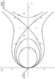
Figure 1: Phase portrait of the invariant plane $M=N=R,p_{M}=p_{N}=p_{R}$, in the coordinates $(x,p_{x})$ defined by $(21)-(22)$. The separatrices S are characterized by the energy $E_{0}=E_{crit}=\frac{1}{4\sqrt{\Lambda}}$. $E$ is the critical point of saddle-center-center type, that belongs to the invariant plane (cf. text). $x=0,p_{x}=0$ is the FRW singularity.

To proceed with the study of the phase space dynamics, let us now linearize the dynamical equations (Homoclinic Chaos in the Dynamics of a General Bianchi IX Model), (Homoclinic Chaos in the Dynamics of a General Bianchi IX Model) about the critical point E. We define

$$X = (M-M_{0}),W=(p_{M}-0),$$

$$Y = (N-M_{0}),K=(p_{N}-0),$$ (8)

$$Z = (R-R_{0}),L=(p_{R}-0).$$

We obtain

$$\left(\begin{array}[]{c}\dot{X}\\ \dot{Y}\\ \dot{Z}\\ \dot{W}\\ \dot{K}\\ \dot{L}\\ \end{array}\right)=\frac{1}{M_{0}}\ S\left(\begin{array}[]{c}X\\ Y\\ Z\\ W\\ K\\ L\\ \end{array}\right)$$

where

$$\left(\begin{array}[]{cccccc}0&0&0&-1/4&1/4&1/4\\ 0&0&0&1/4&-1/4&1/4\\ 0&0&0&1/4&1/4&-1/4\\ 3&-1&-1&0&0&0\\ -1&3&-1&0&0&0\\ -1&-1&3&0&0&0\end{array}\right)$$

In what follows, without loss of generality, we fix $\Lambda$ such that $M_{0}=1$. The nature of the critical point E is determined by the characteristic polynomial associated with the linearization matrix $S$. We obtain

$$P(\lambda)=({\lambda}^{2}-\frac{1}{4})({\lambda}^{2}+2)^{2},$$ (9)

with roots

$$\lambda=\pm\frac{1}{2},\lambda=\pm i\sqrt{2},$$ (10)

where the second pair has multiplicity two. The pair of real eigenvalues generates a saddle structure, while the degenerate pair of imaginary eigenvalues generate a double center structure. The analysis of the center structure will reveal a manifold of linearized unstable periodic orbits with the topology of a $3$-sphere, as we will see.

To display the structure of the linearized motion, we start by diagonalizing $S$ with the use of a transformation matrix $\Re$ whose columns are composed of six independent eigenvectors of $S$ siegel . A judicious choice of $\Re$ yields primed variables defined by the transformation

$${X}^{\prime} = \frac{1}{3}(X+Y+Z),$$

$${Y}^{\prime} = (X-Y),$$

$${Z}^{\prime} = (X+Y-2Z),$$ (11)

$${W}^{\prime} = (W+K+L),$$

$${K}^{\prime} = \frac{1}{2}(W-K),$$

$${L}^{\prime} = \frac{1}{6}(W+K-2L).$$

In these new variables, the quadratic Hamiltonian about $E$ is expressed in the form

$$H=(E_{crit}-E_{0})+\frac{1}{4}\left(\frac{1}{6}W^{\prime 2}-6X^{\prime 2}\right)$$ (12)

$$-\left(\frac{1}{2}K^{\prime 2}+Y^{\prime 2}\right)-\left(\frac{3}{2}L^{\prime 2}+\frac{1}{3}Z^{\prime 2}\right).$$

These variables are conjugated to the pairs according to $[X^{\prime},W^{\prime}]=1,[K^{\prime},Y^{\prime}]=1,[L^{\prime},Z^{\prime}]=1$, other Poisson brackets (PB) zero. The Hamiltonian (12) is separable, and we can immediately identify the following constants for the linearized motion

$$E_{hyp}=\frac{1}{4}\left(\frac{1}{6}W^{\prime 2}-6X^{\prime 2}\right),$$ (13)

$$E_{rot_{1}}=\frac{3}{2}L^{\prime 2}+\frac{1}{3}Z^{\prime 2},$$ (14)

$$E_{rot_{2}}=\frac{1}{2}K^{\prime 2}+Y^{\prime 2},$$ (15)

$$Q_{1}=\frac{1}{3}Y^{\prime}Z^{\prime}+\frac{1}{2}K^{\prime}L^{\prime},$$ (16)

$$Q_{2}=L^{\prime}Y^{\prime}-\frac{1}{3}Z^{\prime}K^{\prime},$$ (17)

in the sense that they all have zero PB with the Hamiltonian (12). The first three constants appear already as separable pieces in the Hamiltonian (12). $E_{hyp}$ corresponds to the energy associated with motion in the saddle sector, while $E_{rot_{1}}$ and $E_{rot_{2}}$ are the rotational energies associated with the motion in the linear part of the center-center manifold, namely, on stable periodic orbits in 2-dim tori. The remaining two constants are additional symmetries that arise as consequence of the multiplicity two of the imaginary eigenvalues, and are associated to the fact that the linearized dynamics in the center-center sector is that of a two-dimensional isotropic harmonic oscillator. They are not all independent but are related by

$$4E_{rot_{1}}E_{rot_{2}}=12Q_{1}^{2}+6Q_{2}^{2}.$$ (18)

We are now ready to describe the topology of the general dynamics in a linear neighborhood of the critical point $E$. To describe all possible motions, the following situations must be taken into account in the linearized Hamiltonian (12). If $E_{hyp}=0$ two possibilities arise. First, we have ${W}^{\prime}={X}^{\prime}=0$, implying that the motions are periodic orbits of the two-dimensional isotropic harmonic oscillator

$$H=\left(\frac{1}{2}K^{\prime 2}+Y^{\prime 2}\right)+\left(\frac{3}{2}L^{\prime 2}+\frac{1}{3}Z^{\prime 2}\right)$$ (19)

$$=(E_{crit}-E_{0}).$$

By a proper canonical reescaling of the variables in (Homoclinic Chaos in the Dynamics of a General Bianchi IX Model) and (19) it is easy to see that these constant energy surfaces are hyperspheres and that the constants of motion $Q_{1}$, $Q_{2}$ and $Q_{3}=(E_{rot_{1}}-E_{rot_{2}})$ satisfy the algebra of the three dimensional rotation group under the Poisson bracket operation, namely,

$$[Q_{i},Q_{j}]=\epsilon^{ijk}Q_{k}$$ (20)

The constant of motion $Q_{1}$ considered as a generator of infinitesimal contact transformations has a peculiar significance in characterizing the topology of the underlying group of the algebra (20)mcintosh . While $Q_{2}$ generates infinitesimal rotations of the orbits, $Q_{1}$ generates infinitesimal changes in eccentricity. The action of $Q_{1}$ is to take an orbit - let us say nearly circular - and transforms it into an orbit of higher and higher eccentricity until it collapses into a straight line. Continued application of $Q_{1}$ produces again an elliptic orbit, but now traversed in the opposite sense , so that it takes a $720^{0}$ rotation to bring the orbit back into itself. The two-valuedness of the mapping arises from the fact that the orbits are oriented. Therefore we are led to the conclusion that the group generated by these constants of motion is the unitary unimodular group and not the rotation group. It is therefore compatible to consider that the center-center manifold has indeed the topology of a three sphere $S^{3}$. Now the separate conservation of $E_{rot_{1}}$ and $E_{rot_{2}}$ (cf.Eq.(19)) allows us to show that the center-center manifold in the linear neighborhood of $E$ is foliated by Clifford two-dimensional surfaces in $S^{3}$ clifford , namely, two-tori $\Im_{E_{0}}$ contained in the energy surface $E_{0}=const$. Such surfaces, as well as the $S^{3}$ manifold that contains them depend continuously on the parameter $E_{0}$. We remark that these two tori will have limiting configurations which are periodic orbits, whenever $E_{rot_{1}}=0$ or $E_{rot_{2}}=0$, and correspond to the case of maximum eccentricity (for instance, a straight line in the plane $({Y}^{\prime},{Z}^{\prime}))$.

The second possibility will be ${W}^{\prime}=\pm 6{X}^{\prime}$, that defines the linear stable $V_{S}$ and unstable $V_{U}$ manifolds of the saddle-sector. $V_{S}$ and $V_{U}$ limit regions $I$ ($E_{hyp}<0$) and regions $II$ ($E_{hyp}>0$) of motion on hyperbolae which are solutions in the separable saddle-sector (cf. (12)) $E_{hyp}=\frac{1}{4}\left(\frac{1}{6}W^{\prime 2}-6X^{\prime 2}\right)$, (cf. (12)). Note that the saddle-sector depicts the structure of Fig. 1 in the neighborhood of $E$, with $V_{U}$ and $V_{S}$ tangent to the separatrices at $E$ barguine . The direct product of $\Im_{E_{0}}$ with $V_{S}$ and $V_{U}$ generates, in the linear neighborhood of $E$, the structure of stable $(\Im_{E_{0}}\times V_{S})$ and unstable $(\Im_{E_{0}}\times V_{U})$ 3-dim tubes, which coalesce into the two-dimensional tori $\Im_{E_{0}}$ for times going to $+\infty$ or $-\infty$, respectively. The energy of any orbit on these tubes is the same as that of the orbits on the two tori $\Im_{E_{0}}$. These 3-dim tubes are confined inside the 4-dim tubes which are the product of $V_{S}$ and $V_{U}$ by the $S^{3}$ center-center manifold. It is obvious that the existence of the $S^{3}$ center-center manifold is restricted to energy surfaces such that $(E_{crit}-E_{0})>0$. The intersection of the center-center manifold with the energy surface $H=E_{0}$ is in general a three sphere parametrized with $E_{0}$, from which two pairs (one stable and one unstable) of 4-dim tubes emanate (cf. Fig. 2 and caption). More particularly, in the linear neighborhood of $E$ (namely, for $(E_{crit}-E_{0})$ small), two pairs of 3-dim tubes emanate from the Clifford two-dimensional surface $\Im_{E_{0}}$ contained in $S^{3}$. For the case $E_{hyp}\not=0$, the motion is restricted on infinite tubes resulting from the direct product of the hyperbolae, lying in the regions $I$ and $II$ of Fig. 1, with $\Im_{E_{0}}$. A general orbit which visits the neighborhood of $E$ belongs to the general case $E_{hyp}\not=0$, $E_{rot_{1}}\not=0$ and $E_{rot_{2}}\not=0$. In this region the orbits have an oscillatory approach to the 3-dim linear tubes, the closer as $E_{hyp}\rightarrow 0$.

Figure 2: Stable and unstable 4-dimensional tubes emanating from the center-center manifold $S^{3}_{E_{0}}$. They are the nonlinear extension of $S^{3}_{E_{0}}(\Im_{E_{0}})\times V_{S}$ and $S^{3}_{E_{0}}(\Im_{E_{0}})\times V_{U}$ in the neighborhood of $E$.

We remark that the surface of the tubes constitutes a boundary for the general flow and, in the neighborhood of $E$, is defined by $E_{hyp}=0$. Depending on the sign of $E_{hyp}$ the motion will be confined inside the 4-dim tube (for $E_{hyp}<0$) and will correspond to a flow of motion distinct from the one confined outside the tube (for $E_{hyp}>0$). This can be seen from Eq.(12), that can be rewritten

$$E_{rot_{1}}+E_{rot_{2}}-E_{hyp}=(E_{crit}-E_{0}).$$

Let us consider, for instance, a set of initial conditions corresponding to initially expanding universes. Two distinct flows will be associated with these initial conditions, depending whether they are contained inside the tube or outside the tube. A careful examination of Fig. 2 shows us that the flow corresponding to initial conditions inside the stable tube will reach a neighborhood of $E$ and will return towards the FRW singularity inside the unstable tube (with $E_{hyp}<0$), while the flow of orbits associated to initial conditions that are outside the tube will reach the neighborhood of $E$ and escapes towards the DeSitter attractor along the exterior of the unstable tube that is directioned to the right. Also the flow of the stable tube on the bottom right of Fig. 2 will escape towards the DeSitter attractor along the interior of the unstable tube of the top right. We remark that the direction of the separatrices and hyperbolae in the linearized saddle-sector are the topological guide for the flow. Our main interest will rely on the stable and unstable tubes that emerge from the neighborhood of the critical point $E$ towards the FRW singularity and their homoclinic transversal crossings, that constitutes an invariant signature of chaos in the models.

By continuity, the nonlinear extension of the center-center manifold will maintain the topology of the three-sphere $S^{3}$, but will not be decomposable into $E_{rot_{1}}$ and $E_{rot_{2}}$ so that now only the four dimensional tubes with topology $R\times S^{3}$ are meaningful for the nonlinear dynamics.

The extension of the structure of the four dimensional tubes away from the neighborhood of $E$ are now to be examined, and our basic interest will reside in on the stable and unstable pair, $S^{3}_{E_{0}}\times V_{S}$ and $S^{3}_{E_{0}}\times V_{U}$, that leave the neighborhood of $E$ and proceed towards the Friedmann-Robertson-Walker (FRW) singularity of the model. To this end let us consider the two dimensional invariant manifold of the dynamics, defined by Eqs.(5). The two dimensional invariant plane is contained in a six dimensional phase space and it is obvious that, contrary to examples in lower dimensional systems, it does not separate the phase space in two disjoint parts. In fact the general motion about a neighborhood of the invariant plane is an oscillatory flow confined along the interior or the exterior of the four dimensional tubes $R\times S^{3}$, where the invariant plane (or more properly, one of the curves of the invariant plane) may be thought as a structure in the center of the tube, as we proceed to show. To see this, let us introduce the canonical coordinate transformation with the generating function

$$G=(MNR)^{\frac{1}{3}}p_{x}+\frac{M}{N}p_{y}+\frac{MN}{R^{2}}p_{z}$$

where $p_{x}$, $p_{y}$ and $p_{z}$ are the new momenta, resulting in

$$x=(MNR)^{\frac{1}{3}},y=\frac{M}{N},z=\frac{MN}{R^{2}}$$ (21)

and

$$p_{M}=\frac{1}{3}\frac{NR}{(MNR)^{\frac{2}{3}}}p_{x}+\frac{1}{N}p_{y}+\frac{N}{R^{2}}p_{z}$$

$$p_{N}=\frac{1}{3}\frac{NR}{(MNR)^{\frac{2}{3}}}p_{x}-\frac{M}{N^{2}}p_{y}+\frac{M}{R^{2}}p_{z}$$ (22)

$$p_{R}=\frac{1}{3}\frac{NR}{(MNR)^{\frac{2}{3}}}p_{x}-\frac{2MN}{R^{3}}p_{z}.$$

It is worth remarking that the linearization of this canonical transformation about the critical point $E$ yields exactly the linear transformation (Homoclinic Chaos in the Dynamics of a General Bianchi IX Model), and that the variables $(y,p_{y},z,p_{z})$ correspond to the primed variables $({K}^{\prime},{Y}^{\prime},{L}^{\prime},{Z}^{\prime})$ defined on the $S^{3}$ center-center manifold about a linear neighborhood of the critical point. The variable $x$ is obviously the average scale factor of the model. In these new variables, the full Hamiltonian (2) assumes the form

$$H=\frac{1}{24x}p_{x}^{2}-\frac{y^{2}}{2x^{3}}p_{y}^{2}-\frac{3z^{2}}{2x^{3}}p_{z}^{2}$$

$$-\frac{x}{2z^{\frac{4}{3}}}-\frac{1}{2}xz^{\frac{2}{3}}y^{2}-\frac{1}{2y^{2}}xz^{\frac{2}{3}}$$

$$+\frac{x}{yz^{\frac{1}{3}}}+\frac{yx}{z^{\frac{1}{3}}}+xz^{\frac{2}{3}}-2{\Lambda}x^{3}=2E_{0},$$ (23)

and the equations of the invariant plane reduce to

$$y=1,z=1,\quad p_{y}=0=p_{z}.$$ (24)

It is clear that $(x,p_{x})$ are variables defined on the invariant plane, and now the expansion of the Hamiltonian (Homoclinic Chaos in the Dynamics of a General Bianchi IX Model) about the neighborhood of the invariant plane can be easily implemented, producing a linearized Hamiltonian parametrized by the variables $(x(t),p_{x}(t))$ describing the curves in the invariant plane, in analogy with the way we expand a dynamical system about a periodic orbit. We obtain

$$H=\frac{1}{24x}p_{x}^{2}+\frac{3x}{2}-2{\Lambda}x^{3}-\frac{1}{2x^{3}}p_{y}^{2}-\frac{3}{2x^{3}}p_{z}^{2}$$

$$-x(y-1)^{2}-\frac{1}{3}x(z-1)^{2}=2E_{0}$$ (25)

with dynamical equations

$$(\delta y\dot{)}=-\frac{1}{x^{3}}{\delta}p_{y}$$

$$(\delta p_{y}\dot{)}=2x{\delta}y$$

$$(\delta z\dot{)}=-\frac{3}{x^{3}}{\delta}p_{z}$$ (26)

$$(\delta p_{z}\dot{)}=\frac{2x}{3}{\delta}z,$$

where ${\delta}y=y-1$, ${\delta}z=z-1$, ${\delta}p_{y}=p_{y}-0$ and ${\delta}p_{z}=p_{z}-0$. The linearization matrix in (Homoclinic Chaos in the Dynamics of a General Bianchi IX Model) has imaginary eigenvalues, both with multiplicity two, given by $\lambda=\pm\frac{i\sqrt{2}}{x(t)}$, so that in the neighborhood of the invariant plane we have only elliptic modes, namely, the motion is oscillatory about the invariant plane with increasing frequency as the orbits approach $x=0$. Close to the critical point $E$, the motion in the invariant plane is slow, i.e., $(\dot{x},\dot{p_{x}})$ is small. Following an orbit in this plane with diminishing $x$, its phase space speed increases but not faster than the frequency of the surrounding motion in the other four variables. We are thus justified in deriving a qualitative picture for the motion near the invariant plane from an adiabatic approximation for the relevant orbit manifolds. That is, we will assume that the overall geometry of the four dimensional stable and unstable tubes that are asymptotic to the $S^{3}$ center-center manifold can be approximated by the adiabatic deformation of this sphere as $x$ decreases away from the critical point. In this way, we have in the six dimensional phase space the four dimensional tubes of motion $R\times{S^{3}}$ with the two dimensional invariant plane as the structure at its center, about which are the oscillatory degrees of freedom $(y,p_{y},z,p_{z})$. We will use this fact to show that the motion in the invariant plane guides the four dimensional tubes of motion inducing inevitably the crossing of the unstable tube with the stable one in the neighborhood of $(x=0,p_{x}=0)$. Also the eigenvectors of the matrix in (Homoclinic Chaos in the Dynamics of a General Bianchi IX Model) can give us an idea of the behaviour of the flow in the tubes as $x$ diminishes, although in the neighborhood of $x=0$ the linear expansion (Homoclinic Chaos in the Dynamics of a General Bianchi IX Model)-(Homoclinic Chaos in the Dynamics of a General Bianchi IX Model) is no longer valid. Associated with the eigenvalue $\lambda=\frac{i\sqrt{2}}{x}$ we may choose the two independent eigenvectors

$$e_{1} = \left[\frac{1}{x},\frac{2x}{i\sqrt{2}},0,0\right]$$

$$e_{2} = \left[0,0,\frac{1}{x},\frac{2x}{3i\sqrt{2}}\right],$$

and for the eigenvalue $\lambda=-\frac{i\sqrt{2}}{x}$,

$$e_{3} = \left[-\frac{i\sqrt{2}}{2x},x,0,0\right]$$

$$e_{4} = \left[0,0,-\frac{3i\sqrt{2}}{2x},x\right].$$

From the above form of the eigenvectors, we can draw a series of important informations about the behaviour of the four dimensional tubes as they approach the singularity $x=0$. As $x$ decreases, the sections $x=const.$ of the four dimensional tubes about the invariant plane stretches in two directions and contracts in other two, while maintaining their symplectic invariants constant. Also as $x$ decreases the oscillations have increasing instantaneous frequency $\propto\frac{\sqrt{2}}{x}$. This appears as a characteristic of the dynamical approach to the singularity even for the extension of the tubes to a nonlinear neighborhood of the invariant plane. There is a further fundamental fact that results from the $x$-dependence of the above eigenvectors: let us consider for instance the sections $x=1$ of the tubes which emanate from the two-tori $\Im_{E_{0}}$ defined in the linear neighborhood of the critical point $E$. Their image projected on the planes $(y,p_{y})$, $(z,p_{z})$ can be rescaled to small circles that deforms into ellipses, as $x$ is infinitesimally diminished; the ellipse is rotated infinitesimally counterclockwise if the section corresponds to the inferior branch of the curves in the invariant plane ($p_{x}<0$) or clockwise if it corresponds to the superior branch ($p_{x}>0$). This will be fundamental to garantee the transversal crossing of the tubes in the neighborhood of $x=0$, as we will discuss. We must however remark that this conclusion is taken in the adiabatic approximation, namely, considering that the variation of $x$ with time is adiabatic; this certainly does not occur near the singularity but we assume that no drastic change in the dynamics will alter this behaviour for the actual dynamical tubes. We illustrate this numerically in Fig. 3 by depicting the sections $x=0.5$ projected on the planes $(y,p_{y})$. Figs. 4 show a numerical illustration of the unstable and stable 4-dim tubes emanating from the neighborhood of $E$ towards the FRW singularity. We note that, for $E_{crit}-E_{0}$ small, the motion proceeds towards the singularity along a tube whose projection on the invariant plane $(x,p_{x})$ shadows the invariant curve corresponding to $H=E_{0}$, along the upper branch and the lower branch (cf.Fig. 4(b)).

We proceed now to show the homoclinic crossing of the stable and unstable tubes at the neighborhood of the singularity $(x=0,p_{x}=0)$, a phenomenon analogous to Poincaré’s homoclinic tangle, and source of chaos in the modelkoiller . The four following points are essential for this. First, in the five dimensional energy surface $H=E_{0}$, the four dimensional tubes of motion $R\times S^{3}$ actually divide the space, separating the dynamics outside from the dynamics inside the tubes. Second, in the canonical variables $(x,p_{x},y,p_{y},z,p_{z})$ introduced above, we have seen that $(x,p_{x})$ are the variables on the invariant plane, whose phase space picture is depicted in Fig. 1, and the remaining degrees of freedom $(y,p_{y},z,p_{z})$ correspond to elliptic modes of motion (cf. analysis in the neighborhood of the invariant plane). Actually, the tubes have the two dimensional invariant plane as the structure at its center (more properly, one of the curves of the invariant plane corresponding to $H=E_{0}$), about which the flow with the oscillatory degrees of freedom $(y,p_{y},z,p_{z})$ proceeds and in fact the motion in the invariant plane guides the flow, inducing inevitably the crossing of one of the four-dimensional unstable tube with the stable one in a neighborhood of $(x=0,p_{x}=0)$. Third, we note that the invariant plane cannot leave the interior of the four dimensional tubes since they are separation surfaces in the five dimensional manifold $H=E_{0}$, and fourth the property of clockwise rotation or counterclockwise rotation of the sections of the stable and unstable tubes, respectively, in their approach to the FRW singularity. Summing up, in the five dimensional energy surface $H=E_{0}$, the model presents the structure of four dimensional tubes of orbits, emanating from a three sphere along the two saddle directions about the critical point saddle-center-center $E$, one stable and one unstable (the stable one corresponding to initially expanding universes). These tubes have the invariant plane curve as the structure at its center and the motion in the invariant plane guides the oscillatory flow towards the singularity $(x=0,p_{x}=0)$, inducing inevitably the crossing of the unstable tube with the stable one in a neighborhood of the singularity; that the crossing is not just a point comes from the conservation of sympletic areas in Hamiltonian dynamics, and the transversality of the crossing comes from the clockwise or counterclockwise rotation of the sections $(y,p_{y})$ and $(z,p_{z})$ of the stable and unstable tubes, respectively. If we consider the transversal crossing in a section, say $x=const.$, it is not difficult to see that the intersection is a $S^{2}$ manifold. Therefore the intersection manifold will be a 3-dim tube of flow (with topology $R\times S^{2}$) which is contained both in the 4-dim stable tube and in the 4-dim unstable tube, and homoclinic to the $S^{3}$ center-center manifold. It is the equivalent of a homoclinic 1-dim orbit in lower dimensional cases.

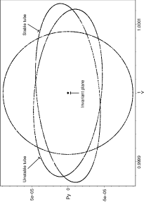
Figure 3: Sections of the stable and unstable tubes projected on the plane $(y,p_{y})$. The dotted circle is the projection of the 2-dim torus $\Im_{E_{0}}$ defined in the linear neighborhood of $E$. The ellipses are the sections for $x=0.5$ of the tubes emanating from $\Im_{E_{0}}$. Note the distortion of the circle into the ellipses and the clockwise/counterclockwise rotation of the sections of the unstable/stable 3-dim tubes as $x$ diminishes (from $x=1$ to $x=0.5$) towards the FRW singularity.

Fig. 4(a)

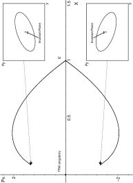
Fig. 4(b)

Figure 4: (a) Numerical illustration of the stable and unstable tubes emanating from the neighborhood of the critical point $E$ towards the FRW singularity, projected on the submanifold $(x,y,p_{x})$, for $E_{crit}-E_{0}=10^{-8}$. (b) Projection of the same stable and unstable tubes of (a) on the invariant plane $(x,p_{x})$. Note that the projection “shadows” the orbits on the invariant plane corresponding to $H=E_{0}$. The insets show the sections $x=0.2$ projected on the $(y,p_{y})$ plane.

Typically, if the 4-dim tubes intersect transversally once they will intersect each other an infinite number of times producing an infinite set of homoclinic orbits which are actually topological 3-dim tubes $R\times S^{2}$. The homoclinic 3-dim tube, which is bi-asymptotic to the $S^{3}$ manifold provides the mechanism for stretching and contraction, giving origin to the homoclinic tangle, which is an invariant signature of chaos in the model wiggins . We just mention that the dynamics near homoclinic orbits is very complex, forming well-known horseshoe structures (cf. wiggins ,koiller ,ozorio and ozorio1 , and the bibliography therein).

Let us consider the first intersection of the tubes; a part of the orbits inside the unstable tube will enter in the interior of the stable tube and the flow will proceed along the stable tube towards the neighborhood of the critical point $E$, from where it will re-enter the unstable tube and proceeds towards the FRW singularity and by a new intersection a part of these orbits will again enter the stable tube and proceed back towards the neighborhood of the critical point $E$, and so on, producing an infinite recurrence of the motion for a class of orbits, which will be periodic orbits of very long periods and bounded oscillatory orbits. Another part of the orbits inside the unstable tube will flow along the exterior of the stable tube towards the neighborhood of the critical point $E$, and afterwards will escape towards the DeSitter attractor at infinity along the exterior of the unstable tube of the second pair (cf. Fig. 2). This for one single intersection. The same pattern will be reproduced for each of the infinite intersections of the unstable tube with the stable one. In this process, the surface of the tubes, which is in fact a boundary for distinct types of flows, will become more and more stretched and folded, resulting in an intricate structure which will have some important physical consequences for the long time behaviour of the orbits. Indeed, basins of initial conditions for initially expanding universes have a fractal boundary associated with recollapse or escape into the DeSitter configuration, as we show soon.

We must comment that the chaotic aspect of the dynamics described here depends crucially on the presence of the cosmological constant that engenders the structure of a saddle-center-center critical point in phase space together with the homoclinic four dimensional tubes, the transversal crossings of which (in a neighborhood of the FRW singularity) characterize chaos definitely and unambiguously in the model. If we restrict ourselves to the energy surface $E_{0}=0$ we have the Mixmaster universe with a cosmological constant which presents the same structure of chaos. For the limiting case ($E_{0}=0,\Lambda=0$), the absence of the critical point appears to eliminate the set of homoclinic orbits and periodic orbits of arbitrarily large periods, whose recurrence engenders chaos in the models. In this instance, our approach does not allow to invariantly characterize chaos in the Mixmaster model.

Our system is open (noncompact) with two definite asymptotic exits, namely, collapse and escape to the DeSitter configuration. The code escape/collapse defines basin boundaries in the initial conditions set; these boundaries are associated precisely to the surface of the homoclinic tubes in the set, and correspond to the initial conditions for the homoclinic intersection manifold contained simultaneously in the stable and in the unstable 4-dim tubes. Together with the countable set of periodic orbits of arbitrarily large periods that exist in the neighborhood of each homoclinic orbit and that have the homoclinic orbit as an accumulation set ozorio ozorio1 , they constitute the set of orbits which neither escape or collapse. This set of bounded orbits that are in the boundary of collapse and escape constitutes , in this way, the strange repellor. The fractal dimension of the basin boundary sets are calculated below by a box-counting method.

Figure 5: Plot of the scaling law $f\propto\epsilon^{\alpha}$ in log-log scale, where $\epsilon$ is the uncertainty radius about 5,000 initial conditions taken inside the set $\cal D$ constructed about the point $(x=0.4,y=1,z=1,p_{x}=2.036467455281656,p_{y}=0,p_{z}=0)$ on the separatrix of the invariant plane $(x,p_{x})$. $f$ is the fraction of $\cal D$ of uncertain initial conditions with respect to the uncertainty code collapse/escape. The set $\cal D$ is a hypercube of edges $10^{-4}$ about the mentioned point, in the energy surface $E_{0}=0.9999999683772234$. The best fit of the small linear region renders $(a)$ $\alpha\approx 0.321$.

In other words, our system has the characteristic of a chaotic scattering system, having the saddle-center-center as a chaotic scatterer, with two absolute outcomes consisting of (i) escape into inflation (the DeSitter attractor) or (ii) recollapse to the singularity, for initially expanding universes. The DeSitter attractor defines a way out from the initial singularity to the inflationary phase but this exit to inflation is completely chaotic, namely, small fluctuations in initial conditions may cause the universe to change its asymptotic behaviour from recollapse to escape into inflation and vice-versa. This is due to the presence of chaotic sets in the phase space of the system, as a consequence of the structure of homoclinic tubes and their transversal crossings, which provides an invariant characterization of chaos in the model. One of the questions to be examined here is the characterization of sets of initial conditions for which the DeSitter attractor is attained and establish the character of a chaotic scattering system. To see this chaotic exit to inflation, let us consider initial conditions sets for initially expanding universes in the energy surface $E_{0}$ such that the orbits visit a linear neighborhood of the saddle-center-center critical point $E$. In this neighborhood, the Hamiltonian is separable according to (12), namely, $H=(E_{crit}-E_{0})+E_{hyp}-E_{rot_{1}}-E_{rot_{2}}=0$. The partition of the energy $(E_{crit}-E_{0})$ into the energies $E_{hyp}$ and $E_{rot_{1}}+E_{rot_{2}}$ of motion about the critical point will determine the outcome of the oscillatory regime about $E$ into collapse or escape to inflation (DeSitter attractor) whether $E_{hyp}<0$ or $E_{hyp}>0$, respectively. However the nonintegrability of the system, with the consequent homoclinic crossing of the tubes, will cause this partition to be chaotic in general, namely, given an arbitrary initial condition of energy $E_{0}$ we are no longer able to foretell in which of regions $I$ or $II$ about the saddle-center the orbit will land when it approaches $E$. Since $E_{hyp}=0$ is a limiting case, for initially expanding universes, the motion inside the tubes corresponds to orbits that will recollapse after reaching the neighborhood of $E$, while the motion outside the tubes corresponds to orbits that will escape into the inflationary phase (towards the DeSitter attractor at infinity). In other words, the intrincate crossing and merging of the tubes produces chaotic sets in the phase space of the model, in particular establishing fractal basin boundaries associated with the chaotic exit to inflation. To illustrate this, we finally present a numerical experiment where we obtain a measure of the fractal dimension of basin boundaries in sets of initial conditions by using the box-counting method with the uncertainty code collapse/escape into inflation. In this numerical experiment we evaluate the fractal dimension of portions $\cal{D}$ of phase space, about a point of the separatrix $S$ on the invariant plane. The box-counting method, due to Ott and collaborators ott , consists of determining the uncertainty exponent $\alpha$ appearing in the scaling law $f\propto\epsilon^{\alpha}$, where $\epsilon$ is the uncertainty radius about 5,000 initial conditions taken inside the sets $\cal{D}$, and $f$ is the fraction of $\cal{D}$ of uncertain initial conditions with the uncertainty code collapse/escape into inflation. The uncertainty exponent is related to the fractal dimension $d$ of the fractal basin boundary by $d=N-\alpha$, where $N=5$ is the phase space energy surface dimensionality. In our numerical experiment we selected a set $\cal{D}$ of homogeneously and randomly distributed initial conditions about the point $(x=0.4,y=1,z=1,p_{x}=2.036467455281656,p_{y}=0,p_{z}=0)$ on the separatrix $S$, such that the orbits visit a neighborhood of the saddle-center-center $E$ before collapse or escape into inflation. In Fig. 5 we depict the scaling law $f\propto\epsilon^{\alpha}$ in which the small linear portion lies between the saturation region for large $\epsilon$ and noise for very small $\epsilon$. The following value for the fractal dimension of the set $\cal{D}$ is found, $d\approx 4.627$, confirming the chaotic nature of these sets.

- (1) V. A. Belinskii, I. M. Khalatnikov and E. M. Lifshitz, Adv. Phys. 19, 525 (1970); Adv. Phys. 31, 639 (1982).
- (2) J. D. Barrow, Phys. Rep. 85, 1 (198); D. F. Chernoff and J. D. Barrow, Phys. Rev. Lett. 50,134 (1983).
- (3) B. K. Berger, Clas. Quant. Grav. 7, 203 (1990); Gen. Rel. Grav. 23, 1385 (1991); Phys. Rev. D49, 1120 (1994).
- (4) B. K. Berger in Deterministic Chaos in General Relativity, eds. D. Hobill, A. Burd and A. Coley (Plenum Press, New York, 1994).
- (5) S. E. Rugh and B. J. T. Jones, Phys. Lett. A147, 353 (1990).
- (6) C. W. Misner. Phys. Rev. Lett. 22, 1071 (1969).
- (7) A. Burd in Deterministic Chaos in General Relativity, eds. D. Hobill, A. Burd and A. Coley (Plenum Press, New York, 1994).
- (8) N. J. Cornish and J. J. Levin, Phys. Rev. D53, 3022 (1996); G. A. Monerat, H. P. de Oliveira and I. Damião Soares, Rev. D58, 063504 (1998).
- (9) H. P. de Oliveira, I. Damião Soares and T. J. Stuchi, Phys. Rev. D56, 730 (1997); R. Barguine, H. P. de Oliveira, I. Damião Soares and E. V. Tonini, Phys. Rev. D63, 063502 (12 pages) (2001).
- (10) Deterministic Chaos in General Relativity, eds. D. Hobill, A. Burd and A. Coley (Plenum Press, New York, 1994).
- (11) A. Latifi, M. Musette and R. Conte, Phys. Lett. A194, 83 (1994).
- (12) G. Contopoulos, B. Grammaticos and A. Ramani, J. Phys. A28, 5313 (1995) .
- (13) G. Francisco and G. E. A. Matsas, Gen. Rel. Grav. 20, 1047 (1998).
- (14) J. N. Cornish and J. J. Levin, Phys. Rev. Lett. 78, 998 (1997); Phys. Rev. D55, 7489 (1997).
- (15) A. E. Motter and P. S. Letelier, Phys. Lett. A285, 127 (2001).
- (16) C. L. Siegel and J. K. Moser, Lectures on Celestial Mechanics (Springer-Verlag, Berlin, 1971).
- (17) H. V. McIntosh, Am. J. Phys. 27, 620 (1959).
- (18) D. M. Y. Sommerville, The Elements of non-Euclidean Geometry (Dover Publication, New York, 1958).
- (19) S. Wiggins, Global Bifurcations and Chaos (Springer-Verlag, Berlin, 1988).
- (20) J. Guckenheimer and P. Holmes, Dynamical Systems and Bifurcations of Vector Fields, Appl. Math. Sciences, Vol.45 (Springer-Verlag, New York, 1983); J. Koiller, J. R. T. de Mello Neto and I. Damião Soares, Phys.Lett. 110A, 260 (1985).
- (21) J. K. Moser, Stable and Random Motions in Dynamical Systems (Princeton University Press, Princeton, NJ, 1973)
- (22) A. M. Ozorio de Almeida, Hamiltonian Systems, Chaos and Quantization (Cambridge University Press, Cambridge, 1988).
- (23) S. Blehar, C. Grebogi, E. Ott and R. Brown, Phys. Rev. A38, 930 (1988); E. Ott, Chaos in Dynamical Systems (Cambridge University Press, Cambridge, 1993).