What can we learn about neutron stars from gravity-wave observations?

Abstract

In the next few years, the first detections of gravity-wave signals using Earth-based interferometric detectors will begin to provide precious new information about the structure and dynamics of compact bodies such as neutron stars. The intrinsic weakness of gravity-wave signals requires a proactive approach to modeling the prospective sources and anticipating the shape of the signals that we seek to detect. Full-blown 3-D numerical simulations of the sources are playing and will play an important role in planning the gravity-wave data-analysis effort. I review some recent analytical and numerical work on neutron stars as sources of gravity waves.

I Introduction

In the course of the next decade, the inception of gravity-wave (GW) astronomy will open an exciting new window on the physics of compact, strongly gravitating objects such as neutron stars (NSs) and black holes (BHs), providing information complementary to that available from electromagnetic and neutrino observations, and plausibly producing important insights into unsolved questions such as the equation of state (EOS) of matter at nuclear densities, and the mechanisms behind gamma-ray bursts. Detailed reviews of GW sources, of the expected event rates, and of the physics that these sources could teach us are available elsewhere,Ferrari ; Hughes ; Kip but I shall list briefly the most promising astrophysical systems from which we could learn about NSs using Earth-based GW interferometers such as LIGO and VIRGO.

1. NS–NS and NS–BH binaries in the last few minutes of their inspirals. For a long time, these inspiraling systems have been the prototype for the category of the short-lived chirp signals detectable using Earth-based interferometers. The reason, of course, is that NS–NS binaries have actually been observed in our galaxy,Thorsett but also that the part of the inspiral accessible to the interferometers (with GW frequencies between 40 and 1000 Hz) sits well before the final merger of the binary, so it is described very accurately by the well-developed post–Newtonian equations for point masses.Blanchet The successful observation of GWs from these events will teach us about the masses, spins and locations of NSs, but not about their internal structure.

   On the contrary, the detection of GW from the endpoint of NS–BH inspirals should produce detailed information about NS structure and EOS. For a wide range of binary parameters, the NS will be torn apart by the tidal field of the BH well before the final plunge into the hole, and the tidal-disruption waves will be well inside the frequency range of good interferometer sensitivity.Vallisneri NS–BH binaries have also been proposed as engines for gamma-ray burstsJanka and as suitable environments for the production of heavy nuclei in $r$-processes.Lee I will discuss these systems more extensively in Sec. II of this paper.

2. Rapidly spinning, deformed NSs. This class includes the known and unknown radio pulsars (when their gravitational ellipticity is high enough to provide strong GWs), and the systems known as low-mass X-ray binaries (LMXB), where the NS is accreting matter and angular momentum from a companion, but instead of increasing its rotation, it is locked into spin periods of about 3 ms; it is conjectured that the angular momentum being accreted is lost to the emission of GW.Bildsten

   To detect rapidly spinning NSs, it will be necessary to integrate the GW signal for times up to several months, so the Doppler frequency modulation caused by the movement of the Earth around the sun will make it much harder to detect previously unknown sources.Brady At the same time, the shape of this modulation will make it possible to obtain the position of the source in the sky,Jaranowski and to match the GW source with one of the objects known from electromagnetic observations.

   If any GWs are detected, their features would be very informative, in particular when examined in correlation with electromagnetic signals from the same source. For instance, the ratio of the GW frequency to the NS angular frequency could identify the nature of the inhomogeneities that give rise to the GW emission, and the evolution of the GW amplitude and frequency could provide interesting data about NS physics such as crust structure and dynamics, crust–core interactions, magnetic fields, viscosity, superfluidity, and more.Kip

3. Proto-neutron stars. Finally, NSs could be observed as the rapidly spinning, strongly asymmetric remnants of stellar-core collapse, or as the proto–NSs produced by the accretion-induced collapse of white dwarves. Proto–NSs that spin very fast can hang up centrifugally at a stage where their radius is still large compared to that of the final NS. Such a configuration might be unstable to a bar mode, giving rise to an elongated object that would emit very strong GWs.bars The newborn NSs might also develop a GW-induced instability in their $r$-modes.Lindblom ; Kokkotas I will discuss this possibility more extensively in Sec. III.

   For all these systems, GWs would provide information complementary to that made available by neutrino observations, focusing on the density structure and asymmetry of the collapsing core rather than on its thermal structure.

While we wait eagerly for the first detections, numerical simulations of GW sources are beginning to provide precious insight into the effect of NS structure and dynamics on the GW signals. The purpose of this paper is to explore how simulations are helping and directing the theory and practice of GW data analysis. To do so, I will single out two promising GW sources (NS tidal disruption in NS–BH binaries, in Sec. II; NS $r$-modes, in Sec. III) that are currently being attacked with numerical simulations, and on which I have first-hand experience.

II Neutron-star tidal disruption as a probe into the equation of state of dense nuclear matter

With event rates between $10^{-7}$ and $10^{-4}$ per year in our galaxy, NS–BH mergers are one of the standard GW sources for second-generation interferometers (LIGO-II should be able to detect these systems out to 650 Mpc, yielding 1–1500 observations per yearKip ). The waveforms generated by these events will contain two kinds of information. The early part of the inspiral (during which the NS and BH are still relatively distant, and the dynamics can be described accurately by post–Newtonian equations of motion in the point-mass approximation) will tell us about the masses and the spins of the NS and BH. The late part of the inspiral, depending on the binary parameters, can see the BH tidal field become so strong that it disrupts the NS on a dynamical timescale; physical intuition then suggests that the details of the disruption process, as encoded in GWs, should carry useful information about the internal structure of the NS, and in particular about its EOS.theidea

II.1 A simple analytical model for NS tidal disruption

The prospects for extracting this information from the GWs that could be measured from a realistic event have been evaluated by the present author,Vallisneri using a crude model that however accounts for most of the relevant physics. The simplest possible representation of a NS inspiraling into a BH is a quasi-equilibrium sequence of relativistic Roche–Riemann ellipsoids. These ellipsoids are equilibrium configurations of a self-gravitating, polytropic, Newtonian fluid, moving on circular, equatorial geodesics in the Kerr spacetime, and subject to the BH relativistic tidal field.Chandra For these configurations, once the binary parameters $m$, $M$, $a$ and $r$ (respectively, the NS and BH masses, the BH spin, and the binary separation) are fixed, there is only one free parameter, corresponding to the NS radius $R$. So we will take $R$ as a representative of the uncertainty in the NS EOS.

As it inspirals toward the BH, a NS with parameters $m$ and $R$ would be represented by the appropriate Roche–Riemann ellipsoid at each separation $r$, until we reach a critical $r_{\mathrm{cr}}$, beyond which no more equilibrium configurations exist. We identify this end of the equilibrium sequence with the onset of dynamical tidal disruption, and from $r_{\mathrm{cr}}$ we obtain the GW frequency at tidal disruption, $f_{\mathrm{td}}=f_{\mathrm{td}}(m,R,M,a)$. This function is shown in Fig. 1, for the standard NS mass $m=1.4\,M_{\odot}$, and for a variety of BH masses. Figure 1 should be read as follows: given a NS–BH signal, choose the curve corresponding to the BH mass (as estimated from the frequency evolution of the early inspiral signal); on the horizontal axis, locate the frequency at which tidal disruption begins (as estimated from the late part of the GW signal); then read off the estimated NS radius on the vertical axis.

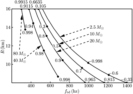
Figure 1: GW frequency at tidal disruption, $f_{\mathrm{td}}(m,R,M,a)$, as a function of NS radius $R$. Here we have set the NS mass to $1.4\,M_{\odot}$, we have indicated the BH mass on the curves, and we have omitted the dependence on the BH spin $a$, which gives negligible corrections. The BH spin parameter $a$ is nevertheless important to decide whether the NS will actually disrupt before it begins its rapid plunge into the BH. Estimating the onset of the plunge as the naive $6M$ ISCO, we find that to have disruption we need $a/M$ to assume at least the value indicated by the big dots in this figure. Negative $a/M$ denotes counterrotating orbits.

Figure 1 suggests that the GW frequency at tidal disruption depends strongly on the NS radius, and that the disruption waveforms lie in the band of good interferometer sensitivity for the advanced interferometers such as LIGO-II. It follows that, in principle, we could use the waveforms from a NS tidal-disruption event to measure both the NS mass and the NS radius. However, we still need to know just how well we could measure them.

II.2 The matched-filtering paradigm for gravity-wave data analysis

To answer this question, we need to invoke the theory of matched-filtering parameter estimation.parest The general idea is that GWs will be detected by correlating the measured signal $|s\rangle$ to a bank of theoretical templates $\{|h_{i}\rangle\}$, which represent our best approximation of the realistic GW signal, as it could happen for a variety of binary parameters. If the match $\langle s|h_{i}\rangle$ (the correlation between $|h_{i}\rangle$ and $|s\rangle$) is much higher than the match $\langle h_{i}|n\rangle$ that the template would give, on the average, with noise alone, then we claim that we have a detection. To know how well we can estimate $R$, we ask how probable it is that a particular realization of detector noise would lead us to mistake the template $|h_{R}\rangle$ with the nearby template $|h_{R+\Delta R}\rangle$: the answer is given in terms of the match $\langle h_{R}|h_{R+\Delta R}\rangle$.

To compute this match we construct a bank of signal templates that differ only in the GW frequency at the onset of tidal disruption. Because we are not interested in modeling accurately the relativistic dynamics of the binary, but only the effects of tidal disruption, we generate our waveforms from simple quadrupole-governed Newtonian inspirals,mtw cutting off the signal, more or less abruptly, when the instantaneous GW frequency reaches $f_{\mathrm{td}}$. Computing the match between nearby templates, we estimate the granularity to which $f_{\mathrm{td}}$ can be measured for a given signal strength (inversely proportional to distance); we can then use our equation for $f(R)$ to propagate the errors to the NS radius. The final result of this exercise is that, employing advanced Earth-based interferometers such as LIGO-IIKip , we should be able to measure the NS radius to 15%, for tidal-disruption events at distances that yield about one event per year.Vallisneri This estimated error should be compared to the error (about a factor of two) in the measurements of the NS thermal radius.

II.3 Inverting the mass–radius relation

What can we do once we get a few points on the $m(R)$ curve? We can try to solve for the EOS of dense nuclear matter in NSs. The relativistic model of nonrotating NSs may be considered as a mapping from the NS EOS, through the Oppenheimer–Volkoff (OV) equations,

$$\frac{dm}{dr}=4\pi r^{2}\rho,\quad\frac{d\rho}{dr}=-(\rho+p)\frac{m+4\pi r^{3}p}{r(r-2m)},$$ (1)

to macroscopic NS quantities such as mass and radius. Let us work through this mapping in the case of a polytropic EOS, $p=p(\rho)$. First, we set the central density $\rho_{c}$; then, we solve the OV equations and compute the NS radius $R=R(\rho_{c})$ and mass $m=m(\rho_{c})$; finally, we eliminate $\rho_{c}$ from these two equations, completing our mapping of the EOS $p(\rho)$ into the mass–radius relation $m(R)$.

Lindblommapping has shown how to invert the OV mapping using even a few $m(R)$ data points. Suppose that $p(\rho)$ is known up to a certain density $\rho_{max}$ from other observations and experiments. Now start with the least dense NS, and integrate the OV equations backward, from the surface of the star [where we know $R$ and $m(R)$] down to the radius where $\rho=\rho_{max}$. We are then left with a stellar core of known mass and radius, and we can use an analytic approximation for the solution of the OV equations to get $p_{c}$ and $\rho_{c}$; we add the point $p_{c}(\rho_{c})$ to the EOS, and repeat for the next NS. The result is $p(\rho)$ as a piecewise linear law. This analysis can be generalized to include rotationally deformed models, and to account for the statistical uncertainty in the $m(R)$ data. Recently, HaradaHarada has shown how other macroscopic parameters of NSs (such as moments of inertia, baryonic masses, binding energies, gravitational redshifts) can be used in this same framework to recover information about the EOS.

Finally, Saijo and NakamuraSaijo have suggested that it might be possible to measure the NS radius directly from the spectrum of the GWs emitted in NS–BH coalescences. These authors have used BH perturbation theory to compute the spectrum of GW emitted by a disk of dust inspiraling into a rotating BH. When the radius $R_{\mathrm{disk}}$ is larger than the wavelength of the quasi-normal modes of the BH, the spectrum acquires several peaks with separation $\propto R_{\mathrm{disk}}^{-1}$, irrespective of $M$ and $a$. Saijo and Nakamura conjecture that the same structure would be visible in the spectrum of GW signals from NS–BH binaries, providing direct information about the radius. However, several issues are left unaddressed: in particular, the particles of the disk move along geodesics, while the fluid of a NS would be strongly constrained by the gravitation and pressure of the star (except, perhaps, in the regime of severe tidal disruption); furthermore, for coalescence events that happen at realistic distances the signal strength might be too low to let us resolve the form-factor structure in the spectrum.

II.4 Numerical simulations of neutron-star tidal disruption

Summarizing, the preliminary analysis carried out by the present author suggests that NS tidal-disruption events have much to teach us about the NS EOS. This prediction is confirmed by Newtonian simulationsCentrella of NS–BH systems, carried out using both smooth particle hydrodynamicsLee ; Lee2 and Eulerian techniquesJanka ; Janka2 , which show that the ultimate fate of the system (complete or incomplete disruption; presence of accretion rings or tidal tails; features of the GW shutoff) depends strongly on the stiffness of the EOS. However, detailed relativistic numerical simulations are still needed to confirm these prospects, and will be essential as a foundation to interpret any tidal-disruption waveforms that might be measured in reality.

III Gravity waves from the $r$-modes of young neutron stars

All rotating stars possess a class of circulation modes ($r$-modes) that are driven toward instability by gravitational radiation reaction; in hot, rapidly rotating young NSs, this destabilizing effect might be so strong that it dominates viscous dissipation. Once an $r$-mode achieves sufficient amplitude, the star is quickly spun down as angular momentum is lost to gravitational radiation.Lindblom ; Kokkotas For stars with initial angular velocity $\Omega\sim 1000$ Hz, the timescale for $r$-mode growth is $\sim 40$ s. In recent years, $r$-modes have attracted considerable interest as a possible explanation for the failure to observe very rapidly spinning pulsars, and as a promising GW source for Earth-based detectors.

However, the astrophysical relevance of $r$-modes is still in doubt, pending judgment on two separate issues. First, the instability of $r$-modes (discovered by analyzing the linearized Euler equations for perfect fluids) might not be confirmed after all the complicated physics that occurs in NSs is taken into account, including relativistic effects, physical-EOS effects, solid crust effects, magnetic fields, rotation laws, and so on. Second, the amount of angular momentum removed from the star and the strength of the GW radiation emitted depend critically on the maximum amplitude that can be reached by the $r$-mode; but the growth of the $r$-mode might be limited to a very small saturation amplitude by the effects of magnetic fieldsRezzolla , or by the leakage of energy to other (damped) modes by way of nonlinear hydrodynamical couplings.

There have been several attempts to investigate the nonlinear dynamics of the $r$-modes, by means of second-order Lagrangian perturbation theory,Teukolsky and of relativistic numerical simulations in the Cowling approximation.Stergioulas In addition, Lindblom, Tohline and the present author have carried out Newtonian numerical simulations that include radiation reaction as an effective force. We now briefly review this work, but we invite the reader to refer to the original articlesrmode1 ; rmode2 for further details.

III.1 Numerical evolutions of nonlinear $r$-modes in neutron stars

We solved the Newtonian Euler and Poisson equations on a $128\times 64\times 128$ cylindrical grid, using a 2nd-order–accurate finite-difference code developed at LSULSU to tackle a variety of astrophysical problems. The LSU code was parallelizedMotl in the domain-decomposition paradigm using the well known MPIMPI library. We ran it on 16 nodes of the HP V-2500 supercomputers at Caltech’s Center for Advanced Computing Research.CACR

Our initial equilibrium configuration was a simple polytrope (with $n=1$, $M=1.4\,M_{\odot}$, $R=12.5$ km) obtained by solving selfconsistently the Bernoulli and Poisson equations.Hachisu We then augmented the rigid-rotation velocity field with a small-amplitude, slow-rotation approximation to an $l=m=2$ $r$-mode,Lindblom98

$$\delta\vec{v}=\alpha_{0}R\Omega_{0}\Bigl{(}\frac{r}{R}\Bigr{)}^{2}\vec{Y}^{B}_{22}e^{i\omega_{0}t},$$ (2)

where $R$ and $\Omega_{0}$ are the radius and angular velocity of the unperturbed star, $\alpha_{0}$ is the dimensionless $r$-mode amplitude, and $\vec{Y}^{B}_{22}$ is a vector spherical harmonic of the magnetic type. Gravitational radiation reaction was added as an effective Newtonian forceforce proportional to the derivatives of the current multipole moments of the star.

Our computing budget set tight limits on the length of the simulation: one full rotation period of a rapidly rotating NS took up to ten thousand CPU hours. Consequently, we could not afford to follow the growth of the $r$-mode through one or more radiation timescales. Instead, we increased the strength of the effective radiation-reaction force by a factor of about 4500, to bring down the $r$-mode growth timescale to values comparable to the rotation period. Even with this trick, we expect that the physical behavior observed in the simulations should still be realistic, because the nonlinear dynamics of the $r$-mode (including its couplings to other modes) should happen at the hydrodynamical timescale, which in our simulations is still much shorter than the radiation-reaction timescale.

Figure 2: Evolution of the dimensionless $r$-mode amplitude $\alpha$. Amplitudes of order one imply mode velocities comparable to the local velocity of rigid rotation. Time is measured in units of the initial rotation period $P_{0}$ of the NS.

While computing the evolution of the star, we monitored the $r$-mode amplitude $\alpha$ by projecting the velocity of the fluid on $\vec{Y}^{B}_{lm}$,

$$\alpha=\frac{2|J_{22}|}{(\Omega/R)\int\rho r^{6}dr},$$ (3)

where $J_{22}$ is the $l=m=2$ current multipole moment; similarly, we read off the mode frequency $\omega$ as

$$\omega=-\frac{1}{|J_{22}|}\left|\frac{d{J}_{22}}{dt}\right|.$$ (4)

At the beginning of our evolution, these diagnostics recovered the theoretical values $\alpha_{0}$ and $\omega_{0}$ within the expected error.

Figure 2 shows the evolution of the $r$-mode amplitude. For this simulation, the theoretical predictionLindblom98 for the $r$-mode growth time was 10 initial rotation periods. The mode grew exponentially (in good accord with theory) until $\alpha\sim 2$; then the mode started to be limited by some nonlinear process, the amplitude peaked at $\alpha=3.35$, and finally fell down very rapidly. A movie of the crashing $r$-mode can be found on the web.vallis

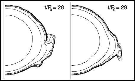
Figure 3: Cresting waves at the surface of the NS, after the $r$-mode amplitude has reached its maximum. The waves create strong shocks that dump mode energy into thermal energy.

What nonlinear process was responsible for limiting the growth of the $r$-mode, and for causing its rapid demise? We discovered a clue when we examined the evolution of the energy and angular momentum in the course of the simulation. Even after the emission of angular momentum into GWs fell to zero, the star continued to lose energy; something other than GWs must be responsible for this loss.

We believe that we have found the culprit. To first order in the amplitude, the $r$-mode is only a velocity mode; to second order, however, there is an associated density perturbation, proportional to $Y_{32}$, which appears as a wave with four crests (two in each hemisphere) on the surface of the star. As the amplitude reaches its maximum, these propagating crests turn into large, breaking waves (see Fig. 3), and the edges of the waves develop strong shocks that dump kinetic energy into thermal energy, killing the $r$-mode.

III.2 Numerical simulations as a laboratory of stellar physics

Our code provided a nice laboratory to perform several more evolutions and tests.

1. We performed basic tests on the robustness of the code and of our diagnostics, evolving stars with different angular velocities, with or without $r$-mode perturbations, and at different grid resolutions.

2. We investigated the dependence of the saturation amplitude on the artificial amplification of radiation reaction. Our computing budget made it impossible to increase the radiation-reaction timescale; instead, we reduced it even more, finding that the $r$-mode saturates faster, but at essentially the same amplitude.

3. We studied the unforced evolution of unit-amplitude $r$-modes, finding that they are essentially stable for as long as we could evolve them. These results are compatible with the relativistic evolutions (also unforced) performed by Stergioulas and Font.Stergioulas

III.3 A new picture for gravity-wave signals from $r$-modes

In the traditional scenario for GW emission from $r$-modes,Owen98 the unstable $r$-mode would grow until it reached a dimensionless amplitude of about one, and then it would saturate and persist at that amplitude (for several months) until it would have lost most of its angular momentum; during that time, the frequency of the $r$-mode would decrease in proportion with the NS spin. The prospective picture of $r$-mode GW signals that emerges from our evolutions is quite different. Most interesting, the $r$-mode spindown episodes are faster (only a few minutes), and the GW frequency remains remarkably constant as the angular velocity of the star decreases. As a result, the search for $r$-mode signals changes from a pulsar-like search (which must account for the Doppler shifts generated by the movement of the Earth around the sun) to an easier chirp-like search, with encouraging prospects for detection.Lindblom01d

Although recent studies of the effect of magnetic fields,Rezzolla and of exotic forms of bulk viscosityLindblom01e suggest that the astrophysical significance of $r$-modes might be limited, the considerable uncertainty about the macroscopic and microscopic structure and dynamics of NSs makes it reasonable to devote some resources to GW searches for $r$-mode signals similar to those predicted by the simulations described above.

- (1) V. Ferrari, proceedings of the 25th J. Hopkins Workshop on Current Problems in Particle Theory. 2001: A Relativistic Spacetime Odyssey, Florence, Sep. 3–5, 2001. astro-ph/0201265.
- (2) S. A. Hughes, S. Márka, P. L. Bender, and C. J. Hogan, proceedings of the 2001 Snowmass Meeting, Snowmass Village, Colorado, June 30–July 21, 2001. astro-ph/0110349.
- (3) K. S. Thorne, “The Scientific Case for Advanced LIGO Interferometers,” LIGO Doc. P-000024-00-D (2001).
- (4) See for instance S. E. Thorsett, and D. Chakrabarty, Astrophys. J. 512, 288 (1999).
- (5) See for instance L. Blanchet, proceedings of the 16th International Conference on General Relativity and Gravitation, Durban, South Africa, July 15–21, 2001. gr-qc/0201050.
- (6) M. Vallisneri, Phys. Rev. Lett. 84, 3519 (2000).
- (7) H.–T. Janka, T. Eberl, M. Ruffert, and C. Fryer, Astrophys. J. 527, L39 (1999).
- (8) W. Lee, MNRAS 318, 606 (2000).
- (9) L. Bildsten, Astrophys. J. Lett. 501, L89 (1998); G. Ushomirsky, C. Cutler, and L. Bildsten, MNRAS 319, 902 (2000), and references therein.
- (10) P. R. Brady, T. Creighton, C. Cutler, and B. F. Schutz, Phys. Rev. D 57, 2101 (1998).
- (11) P. Jaranowski, and A. Krolak, Phys. Rev. D 59, 063003 (1999).
- (12) See for instance M. Shibata, T. W. Baumgarte, and S. L. Shapiro, Astrophys. J. 542, 453 (2000).
- (13) For a recent review, see L. Lindblom, in Gravitational Waves: A Challenge to Theoretical Astrophysics, V. Ferrari, J. C. Miller, and L. Rezzolla, eds. (ICTP, Trieste, 2001). astro-ph/0101136.
- (14) K. D. Kokkotas, proceedings of the 25th J. Hopkins Workshop on Current Problems in Particle Theory. 2001: A Relativistic Spacetime Odyssey, Florence, Sep. 3–5, 2001.
- (15) K. S. Thorne, in Three hundred years of gravitation, S. Hawking and W. Israel, eds. (Cambridge, Cambridge University Press, 1987), p. 330; A. Abramovici, et al., Science 256, 325 (1992).
- (16) S. Chandrasekhar, Ellipsoidal figures of equilibrium (Yale University Press, New Haven, 1969); M. Shibata, Prog. Theor. Phys. 96, 917 (1996); P. Wiggins, and D. Lai, Astrophys. J. 532, 530 (2000).
- (17) See for instance L. S. Finn, Phys. Rev. D 46, 5236 (1992).
- (18) See for instance C. W. Misner, K. S. Thorne, and J. A. Wheeler, Gravitation (W. H. Freeman and Co., San Francisco, 1973).
- (19) L. Bildsten, and C. Cutler, Astrophys. J. 400, 175 (1992).
- (20) L. Lindblom, Astrophys. J. 398, 569 (1992).
- (21) T. Harada, Phys. Rev. C 64, 048801 (2001).
- (22) M. Saijo, and T. Nakamura, Phys. Rev. D 63, 064004 (2001); Phys. Rev. Lett. 85, 2665 (2001).
- (23) For a review of numerical simulations of GW sources, including references to NS–NS and NS–BH simulations, see J. M. Centrella, proceedings the Conference on Stellar Collisions, American Museum of Natural History, June 2000. gr-qc/0011109
- (24) W. Lee, and W. Kluźniak, Acta Astron. 45, 705 (1995); Astrophys. J. Lett. 494, L53 (1998); Astrophys. J. 526, 178 (1999); MNRAS 308, 780 (1999); MNRAS 328, 583 (2001).
- (25) H.–T. Janka, and M. Ruffert, in Proceedings of the 10th workshop on “Nuclear Astrophysics”, W. Hillebrandt and E. Müller, eds. (Garching, Germany, Max-Planck-Institut für Astrophysik, 2000), p. 136.
- (26) L. Rezzolla, F. L. Lamb, D. Markovic, and S. L. Shapiro, Phys. Rev. D 64, 104013 (2001); Phys. Rev. D 64, 104014 (2001).
- (27) A. K. Schenk, P. Arras, É. É. Flanagan, S. A. Teukolsky, and Ira Wasserman, Phys. Rev. D 65, 024001 (2002).
- (28) N. Stergioulas and J. A. Font, Phys. Rev. Lett. 86, 1148 (2001).
- (29) L. Lindblom, J. Tohline and M. Vallisneri, Phys. Rev. Lett. 86, 1152 (2001).
- (30) L. Lindblom, J. Tohline and M. Vallisneri, Phys. Rev. D, in press (2002). astro-ph/0109352.
- (31) K. C. B. New and J. E. Tohline, Astrophys. J. 490, 311 (1997); H. S. Cohl and J. E. Tohline, Astrophys. J. 527, 527 (1999); J. E. Cazes and J. E. Tohline, Astrophys. J. 532, 1051 (2000).
- (32) P. M. Motl, J. Tohline, and J. Frank, Astrophys. J. Suppl. Ser. 138, 121 (2002).
- (33) MPI forum website, www.mpi-forum.org.
- (34) CACR website, www.cacr.caltech.edu.
- (35) I. Hachisu, Astrophys. J. Suppl. Ser. 61, 479 (1986); Astrophys. J. Suppl. Ser. 62, 461 (1986).
- (36) L. Lindblom, B. J. Owen, and S. M. Morsink, Phys. Rev. Lett. 80, 4843 (1998).
- (37) L. Rezzolla, M. Shibata, H. Asada, T. W. Baumgarte, and S. L. Shapiro, Astrophys. J. 525, 935 (1999).
- (38) Michele Vallisneri’s -mode webpage, including movies of the instability, www.vallis.org/rmode.
- (39) B. J. Owen, L. Lindblom, C. Cutler, B. F. Schutz, A. Vecchio, and N. Andersson, Phys. Rev. D 58, 084020 (1998).
- (40) B. J. Owen and L. Lindblom, proceedings, Fourth Amaldi Conference on Gravitational Waves, July 2001, Perth. gr-qc/0111024.
- (41) B. J. Owen and L. Lindblom, Phys. Rev. D, in press (2002). astro-ph/0110558.