Thermodynamics and Kinetic Theory of Relativistic Gases
in 2-D Cosmological Models

Abstract

A kinetic theory of relativistic gases in a two-dimensional space is developed in order to obtain the equilibrium distribution function and the expressions for the fields of energy per particle, pressure, entropy per particle and heat capacities in equilibrium. Furthermore, by using the method of Chapman and Enskog for a kinetic model of the Boltzmann equation the non-equilibrium energy-momentum tensor and the entropy production rate are determined for a universe described by a two-dimensional Robertson-Walker metric. The solutions of the gravitational field equations that consider the non-equilibrium energy-momentum tensor - associated with the coefficient of bulk viscosity - show that opposed to the four-dimensional case, the cosmic scale factor attains a maximum value at a finite time decreasing to a ”big crunch” and that there exists a solution of the gravitational field equations corresponding to a ”false vacuum”. The evolution of the fields of pressure, energy density and entropy production rate with the time is also discussed.

PACS: 51.10.+y; 98.80.-k; 47.75.+f

I Introduction

The combination of general relativity with the kinetic theory of gases is remarkably useful to construct cosmological models Bern . In these formulations the cosmic sources of gravitational interactions are represented by the energy-momentum tensor of a fluid; in addition we have the hypothesis of homogeneity and isotropy in the form of the well-known Robertson-Walker metric Wein1 . Although these theories have explained several important features of our universe fundamental questions still remain to be answered Olive .

Models in lower dimensions offer interesting results that, if properly analyzed, can be used to gain insight in the realistic formulations. Two-dimensional (2-D) gravity models have been under intensive investigation during the last two decades Teit ; Jackiw ; Pol ; Stro ; Mann ; Mann1 . The old problem of quantum gravity, black holes physics and string dynamics were tested in these theories. In particular Teitelboim Teit and Jackiw Jackiw proposed a consistent model in two dimensions analogous of general relativity. As imediate results, among others Jackiw ; Mann , this model offer a consistent Newtonian limit, gravitational collapse solutions that are basically a 2-D Schwarzschild analogue and cosmological models based in a 2-D Robertson-Walker metric.

For cosmological applications, a refinement in the construction of these models can be obtained by considering a non-equilibrium scenario, including a bulk viscosity term in the energy-momentum tensor (for a review on viscous cosmology up to 1990 one is referred to Gron Gron ). In the four-dimensional case the inclusion of this term to analyze the evolution of the cosmic scale factor with the time was done by Murphy Mur who has found a solution that corresponds only to an expansion. Other models were based on the coupling of the Einstein field equations with the balance equations of extended thermodynamics MR (also known as causal or second-order thermodynamic theory) and among others we cite the works of Belinskiǐ et al Bel , Zimdahl Zim and Di Prisco et al Di .

In this work we develop a kinetic theory of relativistic gases in a two-dimensional space. The balance laws for the particle flow, energy-momentum tensor and entropy flow are obtained from the Boltzmann equation. We find also the equilibrium distribution function and the expressions for the fields of energy per particle, pressure, entropy per particle, enthalpy per particle and heat capacities in equilibrium in a two-dimensional space. Moreover, by using the method of Chapman and Enskog for the kinetic model of the Boltzmann equation proposed by Anderson and Witting AW we calculate the bulk viscosity and the entropy production rate. We apply the ideas of Murphy Mur to the 2-D gravitational field equations and we show that opposed to the four-dimensional case the cosmic scale factor attains a maximum value at a finite time decreasing to a ”big crunch” and that there exists a solution of the gravitational field equations corresponding to a ”false vacuum”. The difference between the solutions in the four- and two-dimensional cases is due to the fact that the relationship between the metric tensor and the sources in the 2-D case is modified because the Einstein field equations give no dynamics for the 2-D case.

The manuscript is structured as follows. In Section II we introduce the two-dimensional Robertson-Walker metric. The kinetic theory of relativistic gases in 2-D is developed in Section III. In Section IV we introduce the gravitational equations of motion in the 2-D case and in Section V we search for the solutions of the gravitational field equations. Finally, in Section VI we discuss the solutions that came out from the gravitational field equations.

II Robertson-Walker Metric

One fundamental feature of 2-D cosmological models is that they show considerably less mathematical complexity and at the same time they preserve the physical principles that are used to construct their four-dimensional counterparts. One impressive result was that in 2-D models the quantization of the gravitational field is consistent Jackiw ; Pol , opening the possibility of quantum cosmological models for the very early universe. These results in the 2-D theories are of relevance to include new ingredients in the “realistic” versions Mann ; Mann1 .

As it is well known, the so-called cosmological principle is based on the assumption that the universe is spatially homogeneous and isotropic. The metric that describes such kind of universe, known as the Robertson-Walker metric, has the following form in a two-dimensional Riemannian space characterized by the metric tensor $g^{\mu\nu}$ with signature $(+\,-)$ Mann ; Mann1

$$ds^{2}=(cdt)^{2}-\kappa(t)^{2}{(dr)^{2}\over 1-\varepsilon r^{2}}.$$ (1)

In the above equation $\kappa(t)$ - the so-called cosmic scale factor - is an unknown function of the time and has dimension of length, while $r$ is a dimensionless quantity. If we introduce a new variable $x=\arcsin(\sqrt{\varepsilon}r)/\sqrt{\varepsilon}$ the equation (1) reduces to

$$ds^{2}=(cdt)^{2}-\kappa(t)^{2}(dx)^{2}.$$ (2)

The components and the determinant $g=-\det((g_{\mu\nu}))$ of the metric tensor $g_{\mu\nu}$ for the Robertson-Walker metric (1) with respect to the coordinates $(x^{\mu})=(ct,x)$ are

$$g_{00}=g^{00}=1,\quad g_{11}=-\kappa^{2}={1\over g^{11}},\quad g=\kappa^{2}$$ (3)

The corresponding non-zero Christoffel symbols read

$$\Gamma_{11}^{0}=\dot{\kappa}\kappa,\quad\Gamma_{01}^{1}={\dot{\kappa}\over\kappa}.$$ (4)

where the dot denotes the derivative with respect to the coordinate $x^{0}=ct$. Once the Christoffel symbols are known the non-vanishing components of the Ricci tensor $R_{\mu\nu}=R^{\tau}_{\mu\tau\nu}$ and the curvature scalar $R=g^{\mu\nu}R_{\mu\nu}$ can be calculated and it follows

$$R_{00}={\ddot{\kappa}\over\kappa},\qquad R_{11}=-\ddot{\kappa}\kappa,\qquad R=2{\ddot{\kappa}\over\kappa}.$$ (5)

III Kinetic Theory of Relativistic Gases in 2-D

III.1 Boltzmann equation and fields in equilibrium

We consider a relativistic ideal gas with particles of rest mass $m$ which is described in the phase space by the one-particle distribution function $f(x^{\mu},p^{\mu})$. The momentum $(p^{\mu})=(p^{0},p)$ has a constraint of constant length $g_{\mu\nu}p^{\mu}p^{\mu}=m^{2}c^{2}$ so that $f(x^{\mu},p^{\mu})\equiv f(x,p,t)$.

The evolution equation of the one-particle distribution function in the phase space is described by the Boltzmann equation, which in the presence of a gravitational field is given by CK1 ; Cher

$$p^{\mu}{\partial f\over\partial x^{\mu}}-\Gamma_{\mu\nu}^{1}p^{\mu}p^{\nu}{\partial f\over\partial p}=-{U^{\mu}p_{\mu}\over c^{2}\tau}(f-f^{(0)}),$$ (6)

where $\Gamma^{1}_{\mu\nu}$ is the affine connection. In the right-hand side of the above equation we have replaced the collision term of the Boltzmann equation by the model equation proposed by Anderson and Witting AW , which refers to a relativistic gas in the Landau and Lifshitz description LL . Further $\tau$ is a characteristic time of order of the time between collisions, $f^{(0)}$ is the equilibrium distribution function and $U^{\mu}$ is the two-velocity such that $U^{\mu}U_{\mu}=c^{2}$.

The first moments of the one-particle distribution function are: the particle flow $N^{\mu}$ and the energy-momentum tensor $T^{\mu\nu}$ which are defined by

$$N^{\mu}=c\int p^{\mu}f\,\sqrt{g}{dp\over p_{0}},\qquad T^{\mu\nu}=c\int p^{\mu}p^{\nu}f\,\sqrt{g}{dp\over p_{0}}.$$ (7)

Furthermore, the entropy flow $S^{\mu}$ is defined by

$$S^{\mu}=-kc\int p^{\mu}f\,\ln f\,\sqrt{g}{dp\over p_{0}},$$ (8)

where $k$ is the Boltzmann constant.

The balance equations for the particle flow $N^{\mu}$, energy-momentum tensor $T^{\mu\nu}$ and entropy flux $S^{\mu}$ can be obtained from the Boltzmann equation (6) and read

$${N^{\mu}}_{;\mu}=0,\qquad{T^{\mu\nu}}_{;\mu}=0,\qquad{S^{\mu}}_{;\mu}=\varsigma\geq 0.$$ (9)

Above $\varsigma$ denotes the entropy production rate defined through

$$\varsigma={kU^{\mu}\over c\tau}\int p_{\mu}f^{(0)}\left({f\over f^{(0)}}-1\right)\ln{f\over f^{(0)}}\sqrt{g}{dp\over p_{0}}.$$ (10)

In the Landau and Lifshitz description LL the particle flow and the energy-momentum tensor are decomposed according to

$$N^{\mu}=nU^{\mu}+{\cal J}^{\mu},$$ (11)

$$T^{\mu\nu}=p^{\langle\mu\nu\rangle}-(P+\varpi)\Delta^{\mu\nu}+{en\over c^{2}}U^{\mu}U^{\nu},$$ (12)

where $n$ is the particle number density, $\cal J^{\mu}$ the non-equilibrium part of the particle flow, $p^{\langle\mu\nu\rangle}$ the pressure deviator, i.e., the traceless part of the pressure tensor, $P$ the hydrostatic pressure, $\varpi$ the dynamic pressure, i.e., the non-equilibrium part of the trace of the energy-momentum tensor, $e$ the internal energy per particle and $\Delta^{\mu\nu}$ the projector defined by

$$\Delta^{\mu\nu}=g^{\mu\nu}-{1\over c^{2}}U^{\mu}U^{\nu},\quad\hbox{such that}\quad\Delta^{\mu\nu}U_{\nu}=0,\quad\Delta^{\mu\nu}\Delta_{\nu}^{\sigma}=\Delta^{\mu\sigma},\quad\Delta_{\mu\nu}\Delta^{\mu\nu}=1.$$ (13)

The the non-equilibrium part of the particle flow $\cal J^{\mu}$ and the pressure deviator $p^{\langle\mu\nu\rangle}$ are perpendicular to $U^{\mu}$.

One can also decompose the entropy flow as

$$S^{\mu}=nsU^{\mu}+\phi^{\mu}$$ (14)

where $s$ denotes the entropy per particle and $\phi^{\mu}$ the entropy flux which is perpendicular to $U^{\mu}$.

The equilibrium distribution function in a two-dimensional space, which is the so-called Maxwell-Jüttner distribution function, can be written as

$$f^{(0)}={n\over 2mcK_{1}(\zeta)}e^{-{1\over kT}U^{\mu}p_{\mu}},\qquad\hbox{where}\qquad\zeta={mc^{2}\over kT},$$ (15)

where $T$ denotes the absolute temperature. The parameter $\zeta$ represents the ratio between the rest energy of a particle and the thermal energy of the gas. Moreover, $K_{n}(\zeta)$ denotes the modified Bessel function of second kind (see for example AS )

$$K_{n}(\zeta)=\left({\zeta\over 2}\right)^{n}{\Gamma({1\over 2})\over\Gamma(n+{1\over 2})}\int_{1}^{\infty}e^{-\zeta y}(y^{2}-1)^{n-{1\over 2}}dy.$$ (16)

Once the equilibrium distribution function is known, one can obtain the following expressions for the fields of energy per particle, pressure and entropy per particle in equilibrium:

$$e=mc^{2}\left[{K_{2}(\zeta)\over K_{1}(\zeta)}-{1\over\zeta}\right],\qquad P=nkT,\qquad s_{E}=k\left\{{e\over kT}-\ln\left[{n\over 2mcK_{1}(\zeta)}\right]\right\}.$$ (17)

The thermodynamic quantities enthalpy per particle $h$ and heat capacities per particle at constant volume $c_{v}$ and at constant pressure $c_{p}$ follows from its definitions by using (17), yielding

$$h=e+{P\over n}=mc^{2}{K_{2}(\zeta)\over K_{1}(\zeta)},\quad c_{v}=\left({\partial e\over\partial T}\right)_{v}=k\left[\zeta^{2}+3\zeta{K_{2}(\zeta)\over K_{1}(\zeta)}-\zeta^{2}\left({K_{2}(\zeta)\over K_{1}(\zeta)}\right)^{2}-1\right],$$ (18)

$$c_{p}=\left({\partial h\over\partial T}\right)_{p}=k\left[\zeta^{2}+3\zeta{K_{2}(\zeta)\over K_{1}(\zeta)}-\zeta^{2}\left({K_{2}(\zeta)\over K_{1}(\zeta)}\right)^{2}\right]=c_{v}+k.$$ (19)

The above thermodynamic fields in the non-relativistic limiting case where $\zeta\gg 1$, i.e., for low temperatures, read

$$e\approx mc^{2}+{kT\over 2}\left[1+{3\over 4\zeta}+\dots\right],\qquad s_{E}\approx k\left[{1\over 2}+\ln\sqrt{2\pi mk}+\ln{\sqrt{T}\over n}+{1\over\zeta}+\dots\right],$$ (20)

$$h\approx mc^{2}+{3kT\over 2}\left[1+{3\over 4\zeta}+\dots\right],\quad c_{v}\approx{k\over 2}\left[1+{3\over 2\zeta}-{9\over 4\zeta^{2}}+\dots\right].$$ (21)

In the ultra-relativistic limiting case where $\zeta\ll 1$, i.e., for high temperatures and/or for very small rest mass, we have that the leading term of each thermodynamic field is given by

$$e\approx kT={P\over n},\qquad s_{E}\approx k\left[1+\ln{2kT\over nc}\right],\qquad h\approx 2kT,\qquad c_{v}\approx 3k.$$ (22)

III.2 Dynamic Pressure in a Homogeneous and Isotropic Universe

We shall determine in this section the dynamic pressure and the entropy production rate in a spatially homogeneous and isotropic universe. In the four-dimensional case these topics were discussed by Weinberg Wein within the framework of a phenomenological theory and by Bernstein Bern within the framework of a kinetic theory of gases. Without loss of generality, we shall use here the Anderson and Witting model of the Boltzmann equation (6) in order to simplify the calculations.

We begin by neglecting the space gradients - since we are dealing with a spatially homogeneous and isotropic universe - and by considering a comoving frame where $(U^{\mu})=(c,0)$ in a two-dimensional space. Hence it follows that the Boltzmann equation (6) reduces to

$${\partial f\over\partial x^{0}}-2{\dot{\kappa}\over\kappa}p{\partial f\over\partial p}=-{1\over c\tau}(f-f^{(0)}).$$ (23)

We use now the Chapman and Enskog method (see for example CK1 ) and search for a solution of the Boltzmann equation (23) of the form

$$f=f^{(0)}(1+\phi),$$ (24)

where $f^{(0)}$ is the Maxwell-Jüttner distribution function (15) and $f^{(0)}\phi$ is the deviation from equilibrium of the one-particle distribution function. We insert the above representation into the Boltzmann equation (23) and by taking into account only the derivatives of the Maxwell-Jüttner distribution function we get that the deviation $\phi$ is given by

$$\phi=-c\tau\left({\partial\ln f^{(0)}\over\partial x^{0}}-2{\dot{\kappa}\over\kappa}p{\partial\ln f^{(0)}\over\partial p}\right)$$

$$=-c\tau\left[{\dot{n}\over n}+\left(1-\zeta{K_{2}\over K_{1}}\right){\dot{T}\over T}+{c\over kT}p_{0}{\dot{T}\over T}+{c\over kT}{\dot{\kappa}\over\kappa}{p^{2}\over p_{0}}\right].$$ (25)

For the elimination of $\dot{n}$ and $\dot{T}$ from (25) we use the balance equations of the particle flow and energy-momentum tensor of a non-viscous and non-heat-conducting relativistic gas whose constitutive equations read:

$$N^{\mu}=nU^{\mu},\qquad T^{\mu\nu}=(ne+P){U^{\mu}U^{\nu}\over c^{2}}-Pg^{\mu\nu}.$$ (26)

Insertion of the above representations into the balance equations ${N^{\mu}}_{;\mu}=0$ and ${T^{\mu\nu}}_{;\nu}=0$ lead to

$${1\over\sqrt{g}}{\partial\over\partial x^{\mu}}\left(\sqrt{g}nU^{\mu}\right)=0,$$ (27)

$$-{\partial P\over\partial x^{\nu}}g^{\mu\nu}+{1\over\sqrt{g}}{\partial\over\partial x^{\nu}}\left[\sqrt{g}(ne+P){U^{\mu}U^{\nu}\over c^{2}}\right]+(ne+P)\Gamma_{\lambda\nu}^{\mu}{U^{\lambda}U^{\nu}\over c^{2}}=0.$$ (28)

In a comoving frame (27) becomes

$${\dot{n}\over n}=-{\dot{\kappa}\over\kappa},$$ (29)

while the spatial components of (28) are identically satisfied due to the constraint that all quantities $n,P,e$ and $\kappa$ are only functions of the time coordinate. The temporal component of (28) can be written as

$${\dot{T}\over T}=-{k\over c_{v}}{\dot{\kappa}\over\kappa},$$ (30)

where the heat capacity per particle at constant volume $c_{v}$ is given by (18)₂. Equations (29) and (30) are used to eliminate $\dot{n}$ and $\dot{T}$ from (25), yielding

$$\phi=c\tau\left[1+\left(1-\zeta{K_{2}\over K_{1}}\right){k\over c_{v}}+{c\over c_{v}T}p_{0}-{c\over kT}{p^{2}\over p_{0}}\right]{\dot{\kappa}\over\kappa}.$$ (31)

Once the non-equilibrium distribution function (24) is known it is possible to calculate the projection of the energy-momentum tensor in a comoving frame which corresponds to the sum of the hydrostatic pressure with the dynamic pressure, i.e.,

$$P+\varpi=-\Delta_{\mu\nu}T^{\mu\nu}=-\left(g_{\mu\nu}-{U_{\mu}U_{\nu}\over c^{2}}\right)c\int p^{\mu}p^{\nu}f\sqrt{g}{dp\over p_{0}}=c\kappa^{3}\int p^{2}f{dp\over p_{0}}.$$ (32)

We insert (24) together with (31) into (32) and integrate the resulting equation, yielding

$$\varpi=-\eta c{\dot{\kappa}\over\kappa},\qquad\hbox{where}\qquad\eta=-P\tau\left\{\zeta^{2}\left[{K_{2}\over\zeta K_{1}}-1+{{\rm Ki_{1}}\over K_{1}}\right]-1-{1\over c_{v}}\right\}.$$ (33)

In the above equation ${\rm Ki}_{1}$ denotes the integral for the modified Bessel functions (see Abramowitz and Stegun AS p. 483):

$${\rm Ki}_{n}(\zeta)=\int_{\zeta}^{\infty}{\rm Ki}_{n-1}(t)dt=\int_{0}^{\infty}{e^{-\zeta\cosh t}\over\cosh^{n}t}dt.$$ (34)

Hence we have identified the coefficient of proportionality between $\varpi$ and $c{\dot{\kappa}/\kappa}$ as the bulk viscosity $\eta$. If we compare (33) with the constitutive equation for the dynamic pressure, given in terms of the divergence of the two-velocity, i.e., $\varpi=-\eta{U^{\mu}}_{;\mu}$, we infer that here $c\dot{\kappa}/\kappa$ plays the same role as ${U^{\mu}}_{;\mu}$. Furthermore due to the fact that the bulk viscosity is a positive quantity the dynamic pressure decreases when the universe is expanding ($\dot{\kappa}>0$) while it increases when the universe is contracting ($\dot{\kappa}<0$).

As in the four-dimensional case the coefficient of bulk viscosity vanishes in the non-relativistic and ultra-relativistic limiting cases. This can be seen from Figure 1 where the coefficient of bulk viscosity $\eta\sigma/\sqrt{kTm}$ is plotted versus the parameter $\zeta=mc^{2}/(kT)$. Here we have chosen the following expression for the characteristic time CK3

$$\tau={1\over n\sigma v_{s}},\qquad\hbox{with}\qquad v_{s}=\sqrt{{c^{2}c_{p}kT\over c_{v}h}},$$ (35)

where $\sigma$ is a differential cross-section and $v_{s}$ the adiabatic sound speed.

If we consider that the distribution function is given by (25), i.e., $f=f^{(0)}(1+\phi)$, we can use the approximation $\ln(1+\phi)\approx\phi$ valid for $|\phi|\ll 1$ in order to write the entropy production rate (10) in a comoving frame as

$$\varsigma={k\over\tau}\int f^{(0)}\phi^{2}\sqrt{g}dp.$$ (36)

We insert now (24) together with (31) into (36) and get by integrating the resulting equation

$$\varsigma={\eta c^{2}\over T}\left({\dot{\kappa}\over\kappa}\right)^{2}.$$ (37)

Hence the entropy production rate is connected with the bulk viscosity. Weinberg Wein has derived a similar formula in a four-dimensional space by using a phenomenological theory and has also shown that the bulk viscosity alone could not explain the high entropy of the present microwave background radiation. For more details one is referred to Weinberg Wein ; Wein1 .

IV Gravitational Equations of Motion

Given the sources of our universe it is possible to obtain the equations of motion for the gravitational field in the whole space-time. The starting point is of course, the Einstein theory of gravitation.

As far as we are working in 2-D some fundamental problems appear. In fact, the main point is that the Einstein action in 2-D furnishes no dynamics. In other words the usual left-hand side of Einstein equations of motion that follows by using the Hamilton variational principle

$$R_{\mu\nu}-\frac{1}{2}g_{\mu\nu}R\equiv 0,$$ (38)

are in fact an identity in 2-D. This is related to the gauge invariances of gravitation in 2-D: space-time diffeomorphisms and (local) conformal transformations. With this in mind Teitelboim Teit and Jackiw Jackiw proposed as 2-D action

$$S=\int d^{2}x\sqrt{-g}\left\{N(x)\left[R(x)+8\pi T^{\mu}_{\mu}(x)\right]\right\},$$ (39)

where $T^{\mu}_{\mu}(x)$ is the trace of the energy-momentum tensor. Above we have not taken into account the term that refers to the cosmological constant. Using the variational principle for the auxiliary field $N(x)$ the equation of motion that follow is

$$R(x)=-8\pi T^{\mu}_{\mu}(x),$$ (40)

together with the conservation law ${T^{\mu\nu}}_{;\nu}=0$. Equation (40) relates the curvature scalar with the trace of the energy-momentum tensor.

V Solution of Gravitational Field Equations

The gravitational field equations are obtained from (40) together with ${T^{\mu\nu}}_{;\nu}=0$ and by taking into account the constitutive equation for the energy-momentum tensor $T^{\mu\nu}=\epsilon U^{\mu}U^{\nu}-(P+\varpi)\Delta^{\mu\nu}$ where $\epsilon=ne$ is the energy density. Hence it follows that

$$\ddot{\kappa}=-4\pi(\epsilon-P-\varpi)\kappa,\qquad\dot{\kappa}(\epsilon+P+\varpi)+\kappa\dot{\epsilon}=0.$$ (41)

Since $\varpi=-\eta\dot{\kappa}/\kappa$, the above system is closed if we can relate the pressure $P$ and the coefficient of bulk viscosity $\eta$ to the energy density $\epsilon$. Here we follow Murphy Mur and assume a barotropic equation of state for the pressure and a linear relationship between the coefficient of bulk viscosity and the energy density, so that

$$P=(\gamma-1)\epsilon,\qquad\eta=\alpha\epsilon.$$ (42)

Above $\alpha$ is a constant and $\gamma$ may range from $0\leq\gamma\leq 2$. The value $\gamma=1$ refers to a pure matter (dust), $\gamma=2$ to a pure radiation and $\gamma<1$ to a ”false vacuum”.

If we introduce the Hubble parameter $H=\dot{\kappa}/\kappa$ the field equations (41) can be written thanks to (42) as

$$\dot{H}+H^{2}=4\pi\epsilon(\gamma-2-\alpha H),\qquad H(\gamma-\alpha H)\epsilon+\dot{\epsilon}=0.$$ (43)

The elimination of the energy density of the two above equations leads to an equation for the Hubble parameter that reads

$$(\ddot{H}+2H\dot{H})(\gamma-2-\alpha H)+\alpha\dot{H}(\dot{H}+H^{2})+H(\gamma-2-\alpha H)(\gamma-\alpha H)(\dot{H}+H^{2})=0.$$ (44)

Let us search for a solution of (44) by considering $H=H_{*}=$constant. In this case we get that (44) reduces to $(\gamma-2-\alpha H_{*})(\gamma-\alpha H_{*})H_{*}^{3}=0$ and apart from the trivial solution $H_{*}=0$ we have two other solutions, namely: i) $\alpha=\gamma/H_{*}$ and ii) $\alpha=(\gamma-2)/H_{*}$. Only the first solution is physically possible since $0\leq\gamma\leq 2$.

We proceed to analyze the two energy conditions Haw , namely the weak energy condition which dictates that the energy density is a semi-positive quantity, i.e., $\epsilon\geq 0$ and the strong energy condition which imposes that the inequality $\epsilon+P+\varpi\geq 0$ must hold implying that $H/H_{*}\leq 1$.

We are now ready to determine the solutions of the gravitational field equations. For that end we write the system of equations (41) and (43) as

$$(\gamma-1){\ddot{\kappa}\over\kappa}=4\pi P\left(\gamma-2-\gamma{\dot{\kappa}\over\kappa}\right),\qquad\gamma{\dot{\kappa}\over\kappa}\left(1-{\dot{\kappa}\over\kappa}\right)+{\dot{P}\over P}=0,$$ (45)

$$(\gamma-1)(\dot{H}+H^{2})=4\pi P(\gamma-2-\gamma H),\qquad H\gamma(1-H)P+\dot{P}=0,$$ (46)

respectively, where the cosmic scale factor, the Hubble parameter, the pressure and the time are now taken as dimensionless quantities with respect to $H_{*}$. ¿From the first system of equations (45) one may determine the cosmic scale factor $\kappa(t)$ and the pressure $P(t)$ while from the second one (46) the Hubble parameter $H(t)$ can be obtained. We have chosen two values for $\gamma$, one of them $\gamma=0.5$ correspond to a negative pressure (”false vacuum”) while the other $\gamma=1.5$ implies a positive pressure. For the solutions of the two systems of equations (45) and (46) the following initial conditions were taken into account:

$$\cases{\hbox{for}\quad\gamma=0.5,\quad\hbox{then}\quad H(0)=0.5,\quad\kappa(0)=1,\quad P(0)=-1,\cr\hbox{for}\quad\gamma=1.5,\quad\hbox{then}\quad H(0)=0.5,\quad\kappa(0)=1,\quad P(0)=1.}$$ (47)

In Figures 2 through 5 it is shown the evolution with respect to the time of the cosmic scale factor, the Hubble parameter, the pressure and the energy density which follow from the systems of equations (45) and (46) by taking into account the initial conditions (47) and the barotropic equation of state.

Another important quantity which can be plotted versus the time is the entropy production rate. For the cases where $\gamma>1$ the dimensionless expression for entropy production rate (37) can be written as

$$\varsigma={\gamma H^{2}\over(\gamma-1)\kappa}.$$ (48)

In order to obtain the above equation we have used the equation of state $P=nT$ and the solution of the continuity equation (29) which reads $n\propto 1/\kappa$. In Figure 6 we show the evolution of the entropy production rate with respect to the time.

VI Discussion of the Results

We proceed to discuss the results obtained in the last section. First we call attention to the fact that the period where this theory can be applied is the one where there exists an interaction between radiation and matter. The reason is that in the period of pure radiation the dynamic pressure vanishes while in the period of pure matter (dust) there is no interaction at all. Furthermore the solutions are not valid for all values of the time, since in some period the radiation decouples from matter and we have no more the interaction between the radiation and matter which implies a vanishing dynamic pressure.

In Figure 2 it is plotted the cosmic scale factor as function of the time. We have chosen that at the beginning of this period ($t=0$ by adjusting clocks) the cosmic scale factor is different from zero. We infer from this figure that the cosmic scale factor has a maximum at $t\approx 0.0243$ for $\gamma=1.5$ and at $t\approx 0.0123$ for $\gamma=0.5$. From these points on the cosmic scale factor decreases and tends to zero, i.e., it goes to a ”big crunch”. It is noteworthy to call attention to the fact that the corresponding solution in the four-dimensional case Mur neither have this behavior for the cosmic scale factor nor admit a ”false vacuum” solution. As was previously pointed out the difference between the solutions in the four- and two-dimensional cases is due to the fact that the relationship between the metric tensor and the sources in the 2-D case is modified because the Einstein field equations give no dynamics for the 2-D case.

The Hubble parameter as a function of the time is shown in Figure 3. For both values of $\gamma$ the Hubble parameter decrease, attain a zero value for a time which correspond to the maximum of the cosmic scale factor and assume negatives values.

In Figures 4 and 5 the evolution of the pressure and of the energy density are represented as functions of the time, respectively. Both functions decrease with the time and attain their minimum values at the times where the cosmic scale factor has its maximum value. Since in this theory there exists no mechanism that could increase the pressure and the energy density, we infer that the solutions for $t{{}^{>}_{\sim}}0.0243$ when $\gamma=1.5$ and for $t{{}^{>}_{\sim}}0.0123$ when $\gamma=0.5$ are not physically possible. The same conclusion can be drawn out from Figure 6 where the evolution of the entropy production rate is plotted as a function of the time. From this figure we note that the entropy production rate decreases with the time and attains its minimum ($\varsigma=0$) when the cosmic scale factor reach its maximum value. At this point the entropy per particle $s$ attains its maximum value since $nDs=\varsigma\geq 0$. There exists no mechanism in this theory that could increase the entropy density rate from its minimum value with a corresponding decrease of the entropy per particle from its maximum value.

Figure Captions

Figure 1: Volume viscosity $\eta\sigma/\sqrt{kTm}$ vs. $\zeta$.

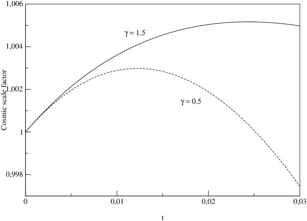
Figure 2: Cosmic scale factor $\kappa(t)$ vs. time $t$.

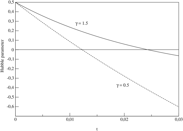
Figure 3: Hubble parameter $H(t)$ vs. time $t$.

Figure 4: Pressure $P(t)$ vs. time $t$.

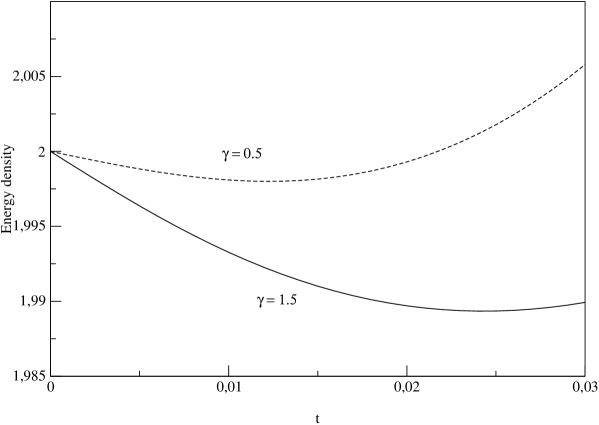
Figure 5: Energy density $\epsilon(t)$ vs. time $t$.

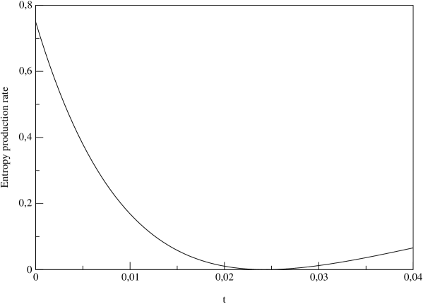
Figure 6: Entropy production rate $\varsigma(t)$ vs. time $t$.

Figure 1: Volume viscosity $\eta\sigma/\sqrt{kTm}$ vs. $\zeta$.

Figure 2: Cosmic scale factor $\kappa(t)$ vs. time $t$.

Figure 3: Hubble parameter $H(t)$ vs. time $t$.

Figure 4: Pressure $P(t)$ vs. time $t$.

Figure 5: Energy density $\epsilon(t)$ vs. time $t$.

Figure 6: Entropy production rate $\varsigma(t)$ vs. time $t$.

References

- (1) J. Bernstein, Kinetic theory in the expanding universe (Cambridge UP, Cambridge, 1988).
- (2) S. Weinberg, Gravitation and cosmology. Principles and applications of the theory of relativity (Wiley, New York, 1972).
- (3) D. E. Groom et al, European Physical Journal C15 , 1 (2000).
- (4) C. Teitelboim, Phys. Lett. B 126, 41 (1983); C. Teitelboim, in Quantum Theory of Gravity, ed. S. Christensen (Adam Hilger, Bristol, 1984) p. 327.
- (5) R. Jackiw, in Quantum Theory of Gravity, ed. S. Christensen (Adam Hilger, Bristol, 1984) p. 403; R. Jackiw, Nucl. Phys. B 252, 343 (1985); J. D. Brown, Lower dimensional gravity, World Scientific, Singapore, 1988. .
- (6) A. M. Polyakov, Mod. Phys. Lett. A 2, 893 (1987).
- (7) C. G. Callan, S. B. Giddings, J. A. Harvey and A. Strominger, Phys. Rev. D 45, 1005 (1992).
- (8) R. B. Mann and S. F. Ross, Phys. Rev. D 47, 3312 (1993).
- (9) K. C. K. Chan and R. B. Mann, Class. Quant. Grav. 10, 913 (1993).
- (10) O. Gron, Astrophys. Space Sci. 173, 191 (1990).
- (11) G. L. Murphy, Phys. Rev. D 8, 4231 (1973).
- (12) I. Müller and T. Ruggeri, Rational extended thermodynamics (Springer, New York, 1998).
- (13) V. A. Belinskiǐ, E. S. Nikomarov and I. M. Khalatnikov, Sov. Phys. JETP 50, 213 (1979).
- (14) W. Zimdahl, Phys. Rev. D 61, 083511 (2000).
- (15) A. Di Prisco, L. Herrera and J. Ibáñez, Phys. Rev. D 63, 023501 (2000).
- (16) J. L. Anderson and H. R. Witting, Physica A 74, 466 (1974).
- (17) C. Cercignani and G. M. Kremer, The relativistic Boltzmann equation: theory and applications (Birkhäuser, Basel, forthcoming 2002).
- (18) N. A. Chernikov, Acta Phys. Polon. 23, 629 (1963).
- (19) L. Landau and E. M. Lifshitz, Fluid mechanics (Pergamon, Oxford, 1987).
- (20) M. Abramowitz and I. A. Stegun, Handbook of mathematical functions (Dover, New York, 1968).
- (21) S. Weinberg, Ap. J. 168, 175 (1971).
- (22) C. Cercignani and G. M. Kremer, Physica A 290, 192 (2001).
- (23) S. W. Hawking and G. F. R. Ellis, The large scale structure of spacetime (Cambridge UP, Cambridge, 1973).