Can Reissner-Nordström wormholes be considered for Spacetime Foam formation?

Abstract

A simple model of spacetime foam, made by $N$ Reissner-Nordström wormholes with a magnetic and electric charge in a semiclassical approximation, is taken under examination. The Casimir-like energy of the quantum fluctuation of such a model is computed and compared with that one obtained with a foamy space modeled by $N$ Schwarzschild wormholes. The comparison leads to the conclusion that a foamy spacetime cannot be considered as a collection of $N$ Reissner-Nordström wormholes but that such a collection can be taken as an excited state of the foam.

I Introduction

Among the long-standing problems in physics, a fundamental one, from a theoretical point of view, is the absence of a quantum theory of gravity. Even if a lot of work has been devoted, especially in the direction of string theory and subsequent modifications, i.e. the branes, a complete scheme is still lacking. On the other hand in the traditional path integral approach to quantum gravity, a typical problem is that the generating functional

$$\int{\cal D}\left[g_{\mu\nu}\right]\exp iS_{g}\left[g_{\mu\nu}\right]$$ (1)

is ill defined because ${\cal D}\left[g_{\mu\nu}\right]$ does not represent a measure and moreover there is no convergence. However, in the context of a WKB approximation with a fixed background, one can obtain interesting informations. Indeed, if one considers a background $\bar{g}_{\mu\nu}$, the gravitational field splits into

$$g_{\mu\nu}=\bar{g}_{\mu\nu}+h_{\mu\nu},$$ (2)

where $h_{\mu\nu}$ is a quantum fluctuation around the background field. Then Eq. $\left(\ref{p01}\right)$ becomes

$$\int{\cal D}g_{\mu\nu}\exp iS_{g}\left[g_{\mu\nu}\right]\simeq\exp iS_{g}\left[\bar{g}_{\mu\nu}\right]\int{\cal D}h_{\mu\nu}\exp iS_{g}^{\left(2\right)}\left[h_{\mu\nu}\right],$$ (3)

where $S_{g}^{\left(2\right)}\left[h_{\mu\nu}\right]$ is the action approximated to second order. In the context of the Euclidean path integration, last expression becomes

$$\int{\cal D}g_{\mu\nu}\exp\left(-I_{g}\left[g_{\mu\nu}\right]\right)\simeq\exp\left(-I_{g}\left[\bar{g}_{\mu\nu}\right]\right)\int{\cal D}h_{\mu\nu}\exp\left(-I_{g}^{\left(2\right)}\left[h_{\mu\nu}\right]\right).$$ (4)

Previous equation can be cast in the form

$$\Gamma=A\exp\left(-I_{cl}\right),$$ (5)

where $\Gamma$ is the decay probability per unit volume and time, while $A$ is the prefactor coming from the saddle point evaluation and $I_{cl}$ is the classical part of the action. If a single negative eigenvalue appears in the prefactor $A$, it means that the related bounce shifts the energy of the false ground state[1]. In particular, it is possible to discuss decay probabilities from one spacetime to another one [2, 3, 4, 5, 6, 7]. For certain classes of gravitational backgrounds, namely the static spherically symmetric metrics, it could be interesting the use of other methods based on variational approach. In a series of papers, we have used such an approach to show that a model of spacetime foam can be concretely realized if one considers a collection of Schwarzschild wormholes whose energy is given by a Casimir energy[9, 10, 11, 12, 13]. We recall that the Casimir energy involves a subtraction procedure between zero point energies having the same boundary conditions. In this paper we would like to apply such methods to another class of static spherically symmetric wormholes involving the electromagnetic field. This class is described by the Reissner-Nordström (RN) metric which is a solution of the Einstein-Maxwell equations with two basic parameters: a mass $M$ and a charge $Q$. Together with the Schwarzschild metric also the RN metric shares the property of being asymptotically flat. This means that the Casimir energy computation for such wormholes class will be made with flat space as a reference space. The final expression will be compared with that one obtained for the Schwarzschild wormholes showing that the Casimir energy for RN wormholes is always higher than the Casimir energy for the Schwarzschild wormholes. This means that RN wormholes cannot be taken as a representation of the ground state of a foamy spacetime. To this purpose we will fix our attention to the following quantity

$$E^{RN}\left(M,Q\right)=E^{flat}\left(0\right)+\Delta E_{flat}^{RN}\left(M,Q\right)_{|classical}+\Delta E_{flat}^{RN}\left(M,Q\right)_{|1-loop},$$ (6)

representing the total energy computed to one-loop in a RN background. $E^{flat}\left(0\right)$ is the reference space energy, which in this case is flat space. $\Delta E_{flat}^{RN}\left(M,Q\right)_{|classical}$ is the energy difference between the RN and the flat metrics, stored in the boundaries and $\Delta E_{flat}^{RN}\left(M,Q\right)_{|1-loop}$ is the quantum correction to the classical term. The analogy between $\Delta E_{flat}^{RN}\left(M,Q\right)_{|1-loop}$ and the prefactor of Eq.$\left(\ref{p02}\right)$ is the key to obtain information about instability. Indeed if we discover that the spectrum of the second order differential operator associated with the quantum fluctuations of transverse and traceless tensors (TT) admits bound states, then we have instability. In this paper we will assume that only one unstable mode appears in the spectrum of TT tensors; this is sufficient to apply Coleman arguments about transition from a vacuum to another one. Note that with this assumption we are in the worst situation, namely the Schwarzschild and RN wormholes can be compared. In fact without the negative mode a spontaneous transition from vacuum to vacuum cannot happen. Therefore in this framework, it is sufficient to compute the stable part of the Casimir energy to compare these different pictures. To concretely compute Eq.$\left(\ref{i0}\right)$ we refer to the following Hamiltonian with boundary

$$H_{T}=H_{\Sigma}+H_{\partial\Sigma}=\int_{\Sigma}d^{3}x\left(N{\cal H+}N_{i}{\cal H}^{i}\right)+H_{\partial\Sigma},$$ (7)

where $N$ is the lapse function, $N_{i}$ is the shift function and

$$\left\{\begin{array}[]{l}{\cal H}{\bf=}G_{ijkl}\pi^{ij}\pi^{kl}\left(\frac{16\pi G}{\sqrt{g}}\right)-\frac{\sqrt{g}}{16\pi G}R^{\left(3\right)}+{\cal H}_{M}\\ {\cal H}^{i}=-2\pi_{|j}^{ij}+{\cal H}_{M}^{i}.\end{array}\right.$$ (8)

${\cal H}_{M}$ is the energy-momentum tensor contribution of the electromagnetic field. $H_{\partial\Sigma}$ represents the energy stored into the boundary. Since the metric considered has no off-diagonal elements, the Hamiltonian becomes

$$H_{T}=H_{\Sigma}+H_{\partial\Sigma}=\int_{\Sigma}d^{3}xN{\cal H}+H_{\partial\Sigma}.$$ (9)

However the physical quantity of interest is the Casimir energy. Therefore we will consider the following expectation value

$$\Delta E_{flat}^{RN}\left(M,Q\right)=\frac{\left\langle\Psi\left|H_{\Sigma}^{RN}-H_{\Sigma}^{flat}\right|\Psi\right\rangle}{\left\langle\Psi|\Psi\right\rangle},$$ (10)

where $H_{\Sigma}^{RN}$ and $H_{\Sigma}^{flat}$ are the total Hamiltonians referred to the RN and flat spacetimes respectively for the volume term[9, 14, 15] and $\Psi$ is a trial wave functional of the gaussian form. Note that the flat space is a particular case of the RN space with the parameters $M=Q=0$. Since the reference space is the same one of the Schwarzschild space, it is immediate to recognize that if an instability appears, flat space could decay via a Schwarzschild black hole pair creation or via a Reissner-Nordström black hole pair creation. Therefore to give indications about the “ground state” of a foamy spacetime, it is important to establish if

$$\Delta E_{flat}^{RN}\left(M,Q\right)\lessgtr\Delta E_{flat}^{Schwarzschild}\left(M\right)$$ (11)

to one-loop approximation. It is important to remark that it is the vacuum energy difference with the same asymptotic reference space that gives the possibility to choose which vacuum is appropriate and not the direct energy difference between these possible candidates. The rest of the paper is structured as follows: in section II, we introduce the Reissner-Nordström metric; in section III, we compute the boundary energy by means of quasilocal energy; in section IV, a variational calculation will be set up to compute the Casimir energy and in particular we will restrict our analysis to the transverse-traceless tensor metric fluctuations (TT); in section V, we evaluate the spectrum of the operator associated with TT tensors (Laplace-Beltrami operator) and we compare the result with what we have obtained in case of Schwarzschild wormholes; in section VI, we summarize and conclude. Units in which $\hbar=c=k=1$ are used throughout the paper.

II The Reissner-Nordström metric

The RN line element is

$$ds^{2}=-f\left(r\right)dt^{2}+f\left(r\right)^{-1}dr^{2}+r^{2}d\Omega^{2},$$ (12)

with

$$f\left(r\right)=\left(1-\frac{2MG}{r}+\frac{Q^{2}}{r^{2}}\right),$$ (13)

where $Q^{2}=G\left(Q_{e}^{2}+Q_{m}^{2}\right)$; $Q_{e}$ and $Q_{m}$ are the electric and magnetic charge respectively. When the electric charge is considered the electromagnetic potential assumes the form $A_{\alpha}=\left(Q_{e}/r,0,0,0\right)$ and the electromagnetic tensor $F_{\alpha\beta}=\partial_{\alpha}A_{\beta}-\partial_{\beta}A_{\alpha}$ is $F_{01}=-Q_{e}/r^{2}$. In the case of a pure magnetic field, the form is $A_{\alpha}=\left(0,-Q_{m}\sin\theta,0,0\right)$ and the electromagnetic tensor becomes $F_{23}=$ $Q_{m}\sin\theta$. Therefore, although the gravitational potential $f\left(r\right)$ assumes the same form, the gravitational perturbation contribute in a different way. When $Q=0$ the metric describes the Schwarzschild metric. When $Q=M=0$, the metric is flat. For $Q\neq 0$, we can distinguish three different cases:

• $MG>Q$. In this case the gravitational potential $f\left(r\right)$ admits two real distinct solutions located at

  $$\left\{\begin{array}[]{c}r_{+}=MG+\sqrt{\left(MG\right)^{2}-Q^{2}}\\ r_{-}=MG-\sqrt{\left(MG\right)^{2}-Q^{2}}\end{array}\right.,$$ (14)

  with $f\left(r\right)>0$ for $r>r_{+}$ and $0<r<r_{-}$ . In the wormhole language, we will say that $r_{-}$ is the inner throat and $r_{+}$ is the outer throat. In the horizon language $r_{-}$ is a Cauchy horizon and $r_{+}$ is an event horizon. For each root there is a surface gravity defined by

  $$\kappa_{\pm}=\lim\limits_{r\rightarrow r_{\pm}}\frac{1}{2}\left|g_{00}^{\prime}\left(r\right)\right|,$$ (15)

  whose values are

  $$\left\{\begin{array}[]{c}\kappa_{+}=\left(r_{+}-r_{-}\right)/2r_{+}^{2}\\ \kappa_{-}=\left(r_{-}-r_{+}\right)/2r_{-}^{2}\end{array}\right.$$ (16)

  and for each surface gravity there exists a bifurcation surface associated to a wormhole throat. The Hawking temperature associated with the surface gravity of the event horizon is

  $$T_{H}=\frac{\kappa_{+}}{2\pi}.$$ (17)

• $MG=Q$. This is the extreme case. The gravitational potential $f\left(r\right)$ admits two real coincident solutions located at $r_{+}=r_{-}=r_{e}=MG$ and its form is $f\left(r\right)=\left(1-MG/r\right)^{2}$. Here we discover that $\kappa_{+}=\kappa_{-}=0$ and $T_{H}=0$.

• $MG<Q$. In this case the gravitational potential $f\left(r\right)$ admits two complex conjugate solutions located at

  $$\left\{\begin{array}[]{c}r_{+,i}=MG+i\sqrt{Q^{2}-\left(MG\right)^{2}}\\ r_{-,i}=MG-i\sqrt{Q^{2}-\left(MG\right)^{2}}\end{array}\right.,$$ (18)

  respectively.

Cases a) and b) imply $Q=0$ when $M=0$. We will restrict our attention on case a) only.

III Quasilocal energy

Quasilocal energy is defined as the value of the Hamiltonian that generates unit time translations orthogonal to the two-dimensional boundary,

$$\Delta E_{Flat}^{RN}\left(M,Q\right)_{|classical}=\frac{1}{8\pi G}\int_{S^{2}}d^{2}x\sqrt{\sigma}\left(k-k^{0}\right),$$ (19)

where $\left|N\right|=1$ at $S^{2}$ and $k^{0}$ is the trace of the extrinsic curvature corresponding to the reference space, which in this case is flat space. The radial coordinate $x$ continuous on ${\cal M}$ is defined by

$$dx=\pm\frac{dr}{\sqrt{1-\frac{2MG}{r}+\frac{Q^{2}}{r^{2}}}},$$ (20)

which in its integrated form becomes

$$x\left(r\right)=\pm\left(r\sqrt{f\left(r\right)}+MG\ln\left(\frac{r-MG+r\sqrt{f\left(r\right)}}{\sqrt{\left(MG\right)^{2}-Q^{2}}}\right)\right)$$ (21)

with $x\left(r\right)=0$ when $r=r_{\pm}$. The surfaces located at $r_{+}$ and $r_{-}$ are bifurcation surfaces denoted by $S_{+}^{0}$ and $S_{-}^{0}$, respectively.

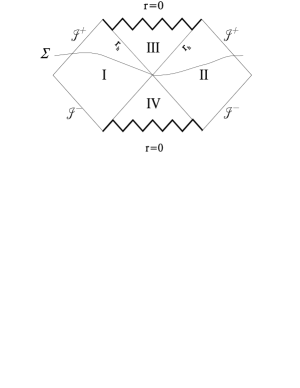
FIG. 1.: Penrose diagram for the Schwarzschild spacetime.

In analogy with the Schwarzschild case, see Fig.1, we will restrict our analysis to the regions I and II of Fig.2, corresponding to the bifurcation surface $S_{+}^{0}$. The constant time hypersurface we will consider will be denoted by $\Sigma_{+}=\Sigma_{++}\cup\Sigma_{+-}$, where the plus sign of Eq.$\left(\ref{p13}\right)$ is relative to $\Sigma_{++}$, while the minus sign is related to $\Sigma_{+-}$. In $\Sigma_{++}$ the evaluation of $\Delta E_{Flat}^{RN}\left(M,Q\right)_{|classical}$ can be obtained as follows: first we consider the static Einstein-Rosen bridge associated to the RN space [17, 18]

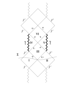
FIG. 2.: Penrose diagram for the Reissner-Nordström spacetime.

$$ds^{2}=-N^{2}\left(r\right)dt^{2}+g_{xx}dx^{2}+r^{2}\left(x\right)d\Omega^{2},$$ (22)

where $N$, $g_{xx}$, and $r$ are functions of $x$ defined by Eq.$\left(\ref{p13}\right)$. Second, we consider the boundary $S_{++}^{2}$, located at $x\left(r\right)=\bar{x}^{++}\left(R\right)$, and its associated normal $n^{\mu}=\delta_{y}^{\mu}$. The expression of the trace

$$k=-\frac{1}{\sqrt{h}}\left(\sqrt{h}n^{\mu}\right)_{,\mu},$$ (23)

gives for the RN space

$$k^{RN}=-2\frac{r,_{x}}{r}_{|RN}=-2\frac{\sqrt{f\left(r\right)}}{r}_{|RN}=-\frac{2}{r}\sqrt{1-\frac{2MG}{r}+\frac{Q^{2}}{r^{2}}}.$$ (24)

Note that if we make the identification $N^{2}=1-\frac{2MG}{r}+\frac{Q^{2}}{r^{2}}$, the line element $\left(\ref{p14}\right)$ reduces to the RN metric written in another form; for our purposes the form of $N\left(r\right)$ can be left unspecified. Thus the computation of $E_{+}$ gives

$$\Delta E_{Flat}^{RN}\left(M,Q\right)_{|classical}=\frac{1}{8\pi G}\int_{S_{++}^{2}}d\Omega^{2}r^{2}\left[\frac{-2\sqrt{f\left(r\right)}}{r}+\frac{2}{r}\right]_{|r=R}$$ (25)

$$=-\frac{R}{G}\left[\sqrt{1-\frac{2MG}{R}+\frac{Q^{2}}{R^{2}}}-1\right].$$ (26)

When $R\gg 2MG$, (and therefore $R\gg Q$), we obtain

$$\Delta E_{Flat}^{RN}\left(M,Q\right)_{|classical}\simeq-\frac{R}{G}\left[\left(1-\frac{MG}{R}+\frac{Q^{2}}{2R^{2}}\right)-1\right]=M.$$ (27)

As expected, since the RN space is A.F., we have obtained that the classical contribution to the energy is exactly the Arnowitt-Deser-Misner mass (ADM) [19]. Since the RN metric is A.F., the computation of the classical energy term leads to

$$E^{RN}\left(M,Q\right)=E^{Flat}+\Delta E_{Flat}^{RN}\left(M,Q\right)_{|classical}=\Delta E_{Flat}^{RN}\left(M,Q\right)_{|classical},$$ (28)

which can be computed by means of quasilocal energy. Thus in complete analogy with the Schwarzschild case, we conclude that flat space cannot decay into RN space because the associated boundary energy (ADM) is different, for every value of the mass $M$ included the extreme value. However if we look at the whole hypersurface $\Sigma_{+}=\Sigma_{++}\cup\Sigma_{+-}$, the total classical energy becomes

$$E^{RN}\left(M,Q\right)=\Delta E_{Flat}^{RN}\left(M,Q\right)_{|classical}^{+}+\Delta E_{Flat}^{RN}\left(M,Q\right)_{|classical}^{-}$$ (29)

with

$\displaystyle\Delta E_{Flat}^{RN}\left(M,Q\right)_{|classical}^{+}=\frac{1}{8\pi G}\int_{S_{++}^{2}}d^{2}x\sqrt{\sigma}\left(k-k^{0}\right),$

$$\Delta E_{Flat}^{RN}\left(M,Q\right)_{|classical}^{-}=-\frac{1}{8\pi G}\int_{S_{+-}^{2}}d^{2}x\sqrt{\sigma}\left(k-k^{0}\right).$$ (30)

Here the boundaries $S_{++}^{2}$ and $S_{+-}^{2}$ are located in the two disconnected regions ${\cal M}_{++}$ and ${\cal M}_{+-}$ respectively with coordinate values $x=\bar{x}^{++}\left(\bar{x}^{+-}\right)$ and the trace of the extrinsic curvature in both regions is

$$k^{RN}=\left\{\begin{array}[]{c}-2r,_{x}/r\qquad on\ \Sigma_{++}\\ 2r,_{x}/r\qquad on\ \Sigma_{+-}\end{array}\right..$$ (31)

Thus one gets

$$\Delta E_{Flat}^{RN}\left(M,Q\right)_{|classical}^{\pm}=\left\{\begin{array}[]{c}M\qquad on\ S_{++}^{2}\\ -M\qquad on\ S_{+-}^{2}\end{array}\right.,$$ (32)

where for $E_{-}$ we have used the conventions relative to $\Sigma_{+-}$ and $S_{+-}^{2}$. Therefore for every value of the boundary $R$, (provided we take symmetric boundary conditions with respect to the bifurcation surface), we have

$$E^{RN}\left(M,Q\right)=M+\left(-M\right)=0,$$ (33)

namely the energy is conserved. As stressed in Ref.[17], since we have a spacetime with a bifurcation surface, the quantities $\Delta E_{Flat}^{RN}\left(M,Q\right)_{|classical}^{+}$ and $\Delta E_{Flat}^{RN}\left(M,Q\right)_{|classical}^{-}$ have the same relative sign, while the total energy is given by the sum $\Delta E_{Flat}^{RN}\left(M,Q\right)_{|classical}^{+}+\Delta E_{Flat}^{RN}\left(M,Q\right)_{|classical}^{-}$. The energies associated to the boundaries are symmetric and they have the same relative sign while the total energy reflects the orientation reversal of the two boundaries. Apparently, Eq.$\left(\ref{p16}\right)$ seems to violate causality, because of the minus appearance in front of the expression. However, as reported in AppendixC, it is such a sign that makes the computation causality preserving. Since the total classical energy is conserved we can discuss the existence of an instability. To this aim we refer to the variational approach to compute the energy density to one-loop[14, 15, 16, 20, 21].

IV Energy Density Calculation in Schrödinger Representation

In previous section we have fixed our attention to the classical part of Eq.$\left(\ref{i0}\right)$. In this section, we apply the same calculation scheme of Refs.[14, 15, 16] to compute one loop corrections to the classical RN term. Like the Schwarzschild case, there appear two classical constraints

$$\left\{\begin{array}[]{l}{\cal H}\text{ }=0\\ {\cal H}^{i}=0\end{array}\right.$$ (34)

and two quantum constraints

$$\left\{\begin{array}[]{l}{\cal H}\tilde{\Psi}\text{ }=0\\ {\cal H}^{i}\tilde{\Psi}=0\end{array}\right.$$ (35)

for the Hamiltonian respectively, which are satisfied both by the RN and flat metric on shell. ${\cal H}\tilde{\Psi}$ $=0$ is known as the Wheeler-DeWitt equation (WDW). Our purpose is the computation of

$$\Delta E_{flat}^{RN}\left(M,Q\right)_{|1-loop}=\frac{\left\langle\Psi\left|H_{\Sigma}^{RN}-H_{\Sigma}^{flat}\right|\Psi\right\rangle}{\left\langle\Psi|\Psi\right\rangle}$$ (36)

where $H_{\Sigma}^{RN}$ and $H_{\Sigma}^{flat}$ are the total Hamiltonians referred to the RN and flat spacetimes respectively for the volume term[9] and $\Psi$ is a wave functional obtained following the usual WKB expansion of the WDW solution. In this context, the approximated wave functional will be substituted by a trial wave functional of the gaussian form according to the variational approach we shall use to evaluate $\Delta E_{flat}^{RN}\left(M,Q\right)_{|1-loop}$. To compute such a quantity we will consider on $\Sigma$ deviations from the RN metric spatial section of the form,

$$g_{ij}=\bar{g}_{ij}+h_{ij},$$ (37)

where

$$\bar{g}_{ij}dx^{i}dx^{j}=\left(1-\frac{2MG}{r}+\frac{Q^{2}}{r^{2}}\right)^{-1}dr^{2}+r^{2}d\Omega^{2}$$ (38)

is the spatial RN background. Thus the expansion of the three-scalar curvature $\int d^{3}x\sqrt{g}R^{\left(3\right)}$ up to $o\left(h^{2}\right)$ gives

$\displaystyle\int_{\Sigma}d^{3}x\sqrt{\bar{g}}\left[-\frac{1}{4}h\triangle h+\frac{1}{4}h^{li}\triangle h_{li}-\frac{1}{2}h^{ij}\nabla_{l}\nabla_{i}h_{j}^{l}+\frac{1}{2}h\nabla_{l}\nabla_{i}h^{li}-\frac{1}{2}h^{ij}R_{ia}h_{j}^{a}+\frac{1}{2}hR_{ij}h^{ij}\right]$

$$+\int_{\Sigma}d^{3}x\sqrt{\bar{g}}\left[\frac{1}{4}h\left(R^{\left(0\right)}\right)h\right],$$ (39)

where $R^{\left(0\right)}$ is the three-scalar curvature on-shell. To explicitly make calculations, we need an orthogonal decomposition for both $\pi_{ij\text{ }}$and $h_{ij}$ to disentangle gauge modes from physical deformations. We define the inner product

$$\left\langle h,k\right\rangle:=\int_{\Sigma}\sqrt{g}G^{ijkl}h_{ij}\left(x\right)k_{kl}\left(x\right)d^{3}x,$$ (40)

by means of the inverse WDW metric $G_{ijkl}$, to have a metric on the space of deformations, i.e. a quadratic form on the tangent space at h, with

$$G^{ijkl}=(g^{ik}g^{jl}+g^{il}g^{jk}-2g^{ij}g^{kl}).$$ (41)

The inverse metric is defined on co-tangent space and it assumes the form

$$\left\langle p,q\right\rangle:=\int_{\Sigma}\sqrt{g}G_{ijkl}p^{ij}\left(x\right)q^{kl}\left(x\right)d^{3}x\text{,}$$ (42)

so that

$$G^{ijnm}G_{nmkl}=\frac{1}{2}\left(\delta_{k}^{i}\delta_{l}^{j}+\delta_{l}^{i}\delta_{k}^{j}\right).$$ (43)

Note that in this scheme the “inverse metric” is actually the WDW metric defined on phase space. Now, we have the desired decomposition on the tangent space of 3-metric deformations[22, 23]:

$$h_{ij}=\frac{1}{3}hg_{ij}+\left(L\xi\right)_{ij}+h_{ij}^{\bot}$$ (44)

where the operator $L$ maps $\xi_{i}$ into symmetric tracefree tensors

$$\left(L\xi\right)_{ij}=\nabla_{i}\xi_{j}+\nabla_{j}\xi_{i}-\frac{2}{3}g_{ij}\left(\nabla\cdot\xi\right).$$ (45)

Then the inner product between three-geometries becomes

$\displaystyle\left\langle h,h\right\rangle:=\int_{\Sigma}\sqrt{g}G^{ijkl}h_{ij}\left(x\right)h_{kl}\left(x\right)d^{3}x=$

$$\int_{\Sigma}\sqrt{g}\left[-\frac{2}{3}h^{2}+\left(L\xi\right)^{ij}\left(L\xi\right)_{ij}+h^{ij\bot}h_{ij}^{\bot}\right].$$ (46)

With the orthogonal decomposition in hand we can define the trial wave functional

$$\Psi\left[h_{ij}\left(\overrightarrow{x}\right)\right]={\cal N}\exp\left\{-\frac{1}{4}\left[\left\langle hK^{-1}h\right\rangle_{x,y}^{\bot}+\left\langle\left(L\xi\right)K^{-1}\left(L\xi\right)\right\rangle_{x,y}^{\|}+\left\langle hK^{-1}h\right\rangle_{x,y}^{Trace}\right]\right\},$$ (47)

where ${\cal N}$ is a normalization factor. Since we are only interested in the perturbations of the physical degrees of freedom, we will only fix our attention on the TT (traceless and transverseless) tensor sector, therefore reducing the previous form into

$$\Psi\left[h_{ij}\left(\overrightarrow{x}\right)\right]={\cal N}\exp\left\{-\frac{1}{4}\left\langle hK^{-1}h\right\rangle_{x,y}^{\bot}\right\}.$$ (48)

This restriction is motivated by the fact that if an instability appears this will be in the physical sector referred to TT tensors, namely a nonconformal instability. This choice seems to be corroborated by the action decomposition of[24], where only TT tensors contribute to the partition function. To calculate the energy density, we need to know the action of some basic operators on $\Psi\left[h_{ij}\right]$[20]. The action of the operator $h_{ij}$ on $|\Psi\rangle=\Psi\left[h_{ij}\right]$ is realized by

$$h_{ij}\left(x\right)|\Psi\rangle=h_{ij}\left(\overrightarrow{x}\right)\Psi\left[h_{ij}\right],$$ (49)

while the action of the operator $\pi_{ij}$ on $|\Psi\rangle$, in general, is

$$\pi_{ij}\left(x\right)|\Psi\rangle=-i\frac{\delta}{\delta h_{ij}\left(\overrightarrow{x}\right)}\Psi\left[h_{ij}\right].$$ (50)

The inner product is defined by the functional integration

$$\left\langle\Psi_{1}\mid\Psi_{2}\right\rangle=\int\left[{\cal D}h_{ij}\right]\Psi_{1}^{\ast}\left\{h_{ij}\right\}\Psi_{2}\left\{h_{kl}\right\}$$ (51)

and by applying previous functional integration rules, we obtain the expression of the one-loop-like Hamiltonian form for TT (traceless and transverseless) deformations[14, 15, 16]

$$H^{\bot}=\frac{1}{4}\int_{{\cal M}}d^{3}x\sqrt{g}G^{ijkl}\left[\left(16\pi G\right)K^{-1\bot}\left(x,x\right)_{ijkl}+\frac{1}{16\pi G}\left(\triangle_{2}\right)_{j}^{a}K^{\bot}\left(x,x\right)_{iakl}\right].$$ (52)

The propagator $K^{\bot}\left(x,x\right)_{iakl}$ comes from a functional integration and it can be represented as

$$K^{\bot}\left(\overrightarrow{x},\overrightarrow{y}\right)_{iakl}:=\sum_{\tau}\frac{h_{ia}^{\bot}\left(\overrightarrow{x}\right)h_{kl}^{\bot}\left(\overrightarrow{y}\right)}{2\lambda\left(\tau\right)},$$ (53)

where $h_{ia}^{\bot}\left(\overrightarrow{x}\right)$ are the eigenfunctions of $\triangle_{2}$. $\tau$ denotes a complete set of indices and $\lambda\left(\tau\right)$ are a set of variational parameters to be determined by the minimization of Eq.$\left(\ref{p22}\right)$.

V The Reissner-Nordström Metric spin 2 operator and the evaluation of the energy density

To evaluate the energy density, we are led to study the following eigenvalue equation

$$\left(\triangle_{2}\right)_{j}^{a}h_{a}^{i}=E^{2}h_{j}^{i}$$ (54)

where $\left(\triangle_{2}\right)_{j}^{a}$ is the Spin-two operator for the RN metric defined by

$$\left(\triangle_{2}\right)_{j}^{a}:=-\triangle\delta_{j}^{a}+2V_{j}^{a}.$$ (55)

$\triangle$ is the curved Laplacian (Laplace-Beltrami operator) on a RN background and $V_{j\text{ }}^{a}$ is defined as

$$V_{j}^{a}:=R_{j}^{a}-P_{j}^{a},$$ (56)

where $R_{j}^{a}$ is the mixed Ricci tensor whose components are:

$$R_{i}^{a}=\left\{-\frac{2MG}{r^{3}}+\frac{2Q^{2}}{r^{4}},\frac{MG}{r^{3}},\frac{MG}{r^{3}}\right\}$$ (57)

and $P_{j}^{a}$ is a mixed tensor coming from the electromagnetic energy-momentum tensor expanded to second order in $h_{ij}$. We will follow Regge and Wheeler in analyzing the equation as modes of definite frequency, angular momentum and parity[26]. The quantum number corresponding to the projection of the angular momentum on the z-axis will be set to zero. This choice will not alter the contribution to the total energy since we are dealing with a spherical symmetric problem. In this case, Regge-Wheeler decomposition shows that the even-parity three-dimensional perturbation is $h_{ij}^{even}\left(r,\vartheta,\phi\right)=$

$$diag\left[H\left(r\right)\left(1-\frac{2MG}{r}+\frac{Q^{2}}{r^{2}}\right)^{-1},r^{2}K\left(r\right),r^{2}\sin^{2}\vartheta K\left(r\right)\right]Y_{l0}\left(\vartheta,\phi\right).$$ (58)

In this representation $H\left(r\right)$ and $K\left(r\right)$ behave as they were scalar fields and the Laplacian restricted to $\Sigma$ is

$$\triangle_{l}=\left(1-\frac{2MG}{r}+\frac{Q^{2}}{r^{2}}\right)\frac{d^{2}}{dr^{2}}+\left(\frac{2r-3MG}{r^{2}}+\frac{Q^{2}}{r^{3}}\right)\frac{d}{dr}-\frac{l\left(l+1\right)}{r^{2}}.$$ (59)

The mixed tensor in Eq. $\left(\ref{p43}\right)$ assumes a different form according to whether we are dealing with the magnetic or electric charge.

A The electric charge contribution

In this case the mixed tensor $P_{j}^{a}$ becomes

$$P_{j}^{a}:=\left(T_{\alpha\beta}u^{\alpha}u^{\beta}\right)\delta_{j}^{a}-\frac{\kappa}{2\pi}\left(F_{01}\right)^{2}\delta_{1}^{a}\delta_{j}^{1}$$ (60)

and for a generic value of the angular momentum $L$, the system $\left(\ref{p41}\right)$ becomes

$$\left\{\begin{array}[]{c}\left(-\triangle_{l}-\frac{4MG}{r^{3}}+\frac{10Q_{e}^{2}}{r^{4}}\right)H_{l}\left(r\right)=E_{l,H}^{2}H_{l}\left(r\right)\\ \\ \left(-\triangle_{l}+\frac{2MG}{r^{3}}-\frac{2Q_{e}^{2}}{r^{4}}\right)K_{l}\left(r\right)=E_{l,K}^{2}K_{l}\left(r\right)\end{array},\right.$$ (61)

where $E_{l,H}^{2}$ and $E_{l,K}^{2}$ are the eigenvalues for the $H_{l}\left(r\right)$ field and the $K_{l}\left(r\right)$ field respectively. Defining reduced fields

$$H_{l}\left(r\right)=\frac{h_{l}\left(r\right)}{r};\qquad K_{l}\left(r\right)=\frac{k_{l}\left(r\right)}{r},$$ (62)

and passing to the proper geodesic distance from the throat of the bridge defined by Eq.$\left(\ref{p13}\right)$, the system $\left(\ref{ep41}\right)$ becomes

$$\left\{\begin{array}[]{c}-\frac{d^{2}}{dx^{2}}h_{l}\left(x\right)+V_{l}^{+}\left(x\right)h_{l}\left(x\right)=E_{l}^{2}h\left(x\right)\\ \\ -\frac{d^{2}}{dx^{2}}k_{l}\left(x\right)+V_{l}^{-}\left(x\right)k_{l}\left(x\right)=E_{l}^{2}k\left(x\right),\end{array}\right.$$ (63)

where

$$V_{l}^{\mp}\left(x\right)=\frac{l\left(l+1\right)}{r^{2}\left(x\right)}\mp\frac{3MG}{r^{3}\left(x\right)}\pm\frac{6Q_{e}^{2}}{r^{4}\left(x\right)}+\frac{3Q_{e}^{2}}{r^{4}\left(x\right)}.$$ (64)

When $r\gg r_{+}$ $x\left(r\right)\simeq r$, then we can approximate the potential with

$$V_{l}^{\mp}\left(x\right)\simeq\frac{l\left(l+1\right)}{x^{2}}$$ (65)

and the solution for the system $\left(\ref{ep42}\right)$ is

$$h_{pl}\left(x\right)=k_{pl}\left(x\right)=\sqrt{\frac{2}{\pi}}\left(px\right)j_{l}\left(px\right),$$ (66)

where $j_{l}\left(px\right)$ is the spherical Bessel function. If we consider flat space, i.e. $M=Q=0$, the system $\left(\ref{ep42}\right)$ becomes

$$\left\{\begin{array}[]{c}\left(-\frac{d^{2}}{dr^{2}}+\frac{l\left(l+1\right)}{r^{2}}\right)h_{l}\left(r\right)=E_{l}^{2}h_{l}\left(r\right)\\ \\ \left(-\frac{d^{2}}{dr^{2}}+\frac{l\left(l+1\right)}{r^{2}}\right)k_{l}\left(r\right)=E_{l}^{2}k_{l}\left(r\right)\end{array}\right.,$$ (67)

and the solution is

$$h_{pl}\left(r\right)=k_{pl}\left(r\right)=\sqrt{\frac{2}{\pi}}\left(pr\right)j_{l}\left(pr\right).$$ (68)

On the other hand when $r\longrightarrow r_{0}>r_{+}$

$$x\left(r\right)\simeq\sqrt{2\kappa_{+}\left(r-r_{+}\right)}\qquad V_{l}^{\mp}\left(x\right)\longrightarrow\frac{l\left(l+1\right)}{r_{0}^{2}}\mp\frac{3MG}{r_{0}^{3}}\pm\frac{6Q_{e}^{2}}{r_{0}^{4}}+\frac{3Q_{e}^{2}}{r_{0}^{4}}=const,$$ (69)

where $\kappa_{+}$ has been defined in Eq. $\left(\ref{p12ab}\right)$. However to use the simplicity of Bessel functions for flat and curved space when $r\longrightarrow r_{0}>r_{+}$, we approximate the potential with

$$V_{l}^{\mp}\left(x\right)=\frac{l\left(l+1\right)}{x^{2}}\mp\frac{3MG}{r_{0}^{3}}\pm\frac{6Q_{e}^{2}}{r_{0}^{4}}+\frac{3Q_{e}^{2}}{r_{0}^{4}}.$$ (70)

Thus close to the wormhole throat we experience a potential barrier (potential hole) whose solution, for system $\left(\ref{ep42}\right)$ is

$$\left\{\begin{array}[]{cc}h_{P_{-}l}\left(x\right)=&\sqrt{\frac{2}{\pi}}\left(P_{-}x\right)j_{l}\left(P_{-}x\right)\\ k_{P_{+}l}\left(x\right)=&\sqrt{\frac{2}{\pi}}\left(P_{+}x\right)j_{l}\left(P_{+}x\right)\end{array}\right..$$ (71)

$P_{\mp}$ is such that $P_{\mp}^{2}=E_{l}^{2}\mp c_{\mp}^{2}$, where

$$c_{\mp}^{2}=\mp\frac{3MG}{r_{0}^{3}}\pm\frac{6Q_{e}^{2}}{r_{0}^{4}}+\frac{3Q_{e}^{2}}{r_{0}^{4}}.$$ (72)

Note that for functions described by Eq.$\left(\ref{ep42aa}\right)$ or Eq.$\left(\ref{ep42ab}\right)$ we have that

$$h_{l}\left(x\right),k_{l}\left(x\right)\rightarrow 0\text{\qquad when\qquad}x\left(r\right)\rightarrow x\left(r_{+}\right)\simeq 0.$$ (73)

Thus the propagator becomes

$$K_{\pm}^{\bot}\left(x,y\right)=\frac{1}{r\left(x\right)r\left(y\right)}\sum_{P,l,m}\left\{\begin{array}[]{c}k_{P_{+}l}\left(x\right)k_{P_{+}l}\left(y\right)/\lambda_{+}\left(P\right)\\ h_{P_{-}l}\left(x\right)h_{P_{-}l}\left(y\right)/\lambda_{-}\left(P\right)\end{array}\right.Y_{l0}\left(\vartheta,\phi\right)Y_{l0}\left(\vartheta^{\prime},\phi^{\prime}\right)$$ (74)

$\lambda_{\pm}\left(P\right)$ is referred to the potential function $V_{l}^{\pm}\left(x\right)$. This is the more general expression for the propagator. Indeed, when one considers flat space or the region far away from the throat $r_{+}$, it is sufficient the substitution of $P_{\mp}$ with $p$. Inserting Eq.$\left(\ref{ep42a}\right)$ into Eq.$\left(\ref{p22}\right)$ one gets

$$E\left(M,Q_{e},\lambda\right)=\frac{1}{2\pi}\sum_{p,l}\frac{\left(2l+1\right)}{4\pi}\sum_{i=1}^{2}\left[\left(16\pi G\right)\lambda_{i}\left(p\right)+\frac{E_{i}^{2}\left(p,M,Q_{e}\right)}{\left(16\pi G\right)\lambda_{i}\left(p\right)}\right]$$ (75)

where

$$\left\{\begin{array}[]{c}E_{1}^{2}\left(p,M,Q_{e}\right)=p^{2}-\frac{3MG}{r_{0}^{3}}+\frac{9Q_{e}^{2}}{r_{0}^{4}}\\ E_{2}^{2}\left(p,M,Q_{e}\right)=p^{2}+\frac{3MG}{r_{0}^{3}}-\frac{3Q_{e}^{2}}{r_{0}^{4}}\end{array}\right.,$$ (76)

$\lambda_{i}\left(p\right)$ are variational parameters corresponding to the eigenvalues for a (graviton) spin-two particle in an external field. By minimizing $\left(\ref{ep42b}\right)$ with respect to $\lambda_{i}\left(p\right)$ one obtains $\overline{\lambda}_{i}\left(p\right)=\left[E_{i}^{2}\left(p,M,Q_{e}\right)\right]^{\frac{1}{2}}/\left(16\pi G\right)$ and

$$E\left(M,Q_{e},\overline{\lambda}\right)=\frac{1}{\pi}\sum_{p,l}\frac{\left(2l+1\right)}{4\pi}\left[\sqrt{E_{1}^{2}\left(p,M,Q_{e}\right)}+\sqrt{E_{2}^{2}\left(p,M,Q_{e}\right)}\right]$$ (77)

with

$$p^{2}+c_{\mp}^{2}>0,$$ (78)

where we have used definition $\left(\ref{ep42ac}\right)$. We can evaluate the total energy for the electric RN background by replacing the sum with an integral leading to

$$E\left(M,Q_{e}\right)=\frac{V}{4\pi^{2}}\int_{0}^{\infty}dpp^{2}\left(\sqrt{p^{2}+c_{-}^{2}}+\sqrt{p^{2}+c_{+}^{2}}\right),$$ (79)

where $V$ is the volume localized near the wormhole throat. For flat space we put $M=Q=0$ and we get

$$E\left(0\right)=\frac{V}{2\pi^{2}}\int_{0}^{\infty}dpp^{3}$$ (80)

Now, we are in position to compute the difference between $\left(\ref{ep42c}\right)$ and $\left(\ref{ep42d}\right)$. The explicit evaluation of the integrals of Eq.$\left(\ref{ep42c}\right)$ in the U.V. limit, gives

$$E\left(M,Q_{e}\right)\simeq\frac{V}{4\pi^{2}}\frac{1}{4}\left[2p^{4}+p^{2}\left(c_{+}^{2}+c_{-}^{2}\right)-\frac{c_{+}^{4}}{4}\ln\left(\frac{p^{2}}{c_{+}^{2}}\right)-\frac{c_{-}^{4}}{4}\ln\left(\frac{p^{2}}{c_{-}^{2}}\right)\right].$$ (81)

Thus

$\displaystyle\Delta E_{flat}^{RN}\left(M,Q_{e}\right)=E\left(M,Q_{e}\right)-E\left(0\right)$

$\displaystyle=\frac{V}{4\pi^{2}}\int_{0}^{\infty}dpp^{2}\left[\sqrt{p^{2}+c_{-}^{2}}+\sqrt{p^{2}+c_{+}^{2}}-2\sqrt{p^{2}}\right]$

$\displaystyle\simeq\frac{V}{4\pi^{2}}\left[\frac{1}{4}p^{2}\left(c_{+}^{2}+c_{-}^{2}\right)-\frac{c_{+}^{4}}{16}\ln\left(\frac{p^{2}}{c_{+}^{2}}\right)-\frac{c_{-}^{4}}{16}\ln\left(\frac{p^{2}}{c_{-}^{2}}\right)\right]$

$$\simeq\frac{V}{4\pi^{2}}\left[\frac{1}{4}p^{2}\left(c_{+}^{2}+c_{-}^{2}\right)-\frac{\left(c_{-}^{4}+c_{+}^{4}\right)}{16}\ln\left(\frac{\Lambda^{2}}{\mu^{2}}\right)\right],$$ (82)

where we have used the approximation $p^{2}>>c_{\mp}^{2}$ and a cut-off $\Lambda\leq m_{p}$ to keep under control the $UV$ divergence and we have introduced an arbitrary scale $\mu$. In particular for the Schwarzschild case, $\mu$ has been determined by the quantity $3MG/r_{0}^{3}=c_{M}^{2}$ and in that case the approximated expression for $\Delta E\left(M\right)$ is

$$\Delta E\left(M\right)\sim-\frac{V}{2\pi^{2}}\frac{c_{M}^{4}}{16}\ln\left(\frac{\Lambda^{2}}{c_{M}^{2}}\right)=-\frac{V}{32\pi^{2}}\left(\frac{3MG}{r_{0}^{3}}\right)^{2}\ln\left(\frac{r_{0}^{3}\Lambda^{2}}{3MG}\right).$$ (83)

Nevertheless, in this paper we would like to establish if a mechanism of space-time foam formation can arise in competition with the foam model created by Schwarzschild wormholes. To this purpose in this case we shall fix as a scale the value $c_{M}^{2}$ and we define the dimensionless parameter $\alpha=\left(Q_{e}/MG\right)$. Thus Eq. $\left(\ref{ep43}\right)$ becomes

$$\Delta E_{flat}^{RN}\left(M,Q_{e}\right)\simeq\frac{V}{4\pi^{2}}\Lambda^{4}\left[\frac{1}{2}x\alpha_{e}^{2}+\frac{1}{16}\left(1+5\alpha_{e}^{4}-4\alpha_{e}^{2}\right)x^{2}\ln x\right]$$ (84)

where we have defined

$$\alpha_{e}^{2}=\alpha^{2}\frac{MG}{r_{0}};\quad x=\frac{3MG}{r_{0}^{3}\Lambda^{2}}.$$ (85)

Since $MG>Q$ and since $r_{0}>MG>Q$ then $0<\alpha_{e}^{2}<1$. In Fig.3, we show the plot of Eq.$\left(\ref{ep43a}\right)$ for different values of the parameter $\alpha_{e}^{2}$.

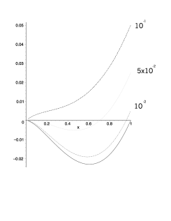
FIG. 3.: Plot of Electric charge contribution for different values of the parameter $\alpha_{e}^{2}$. For $\alpha_{e}^{2}=0$, we have the Schwarzschild space.

Since only the minimum of $\Delta E_{flat}^{RN}\left(M,Q_{e}\right)$ is physically relevant, we see that for $\alpha_{e}^{2}=10^{-1}$, the minimum is positive. This means that the electric field tends to dominate the gravitational attraction and becomes more and more stronger as $\alpha_{e}^{2}$ approaches the extreme value, i.e. $MG=Q_{e}$. As expected for small values of $\alpha_{e}^{2}$, the behavior for the energy gap of the Schwarzschild and RN backgrounds with flat space as reference space are very close. Nevertheless, the energy gap of the last one is always higher than the same one computed with the Schwarzschild background. This means that even for very small electric charges, the Casimir energy for RN wormholes is always higher than the Casimir energy for Schwarzschild wormholes.

B The magnetic charge contribution

For the magnetic case $P_{j\text{ }}^{a}$ is

$$P_{j}^{a}:=\kappa\left(T_{\alpha\beta}u^{\alpha}u^{\beta}\right)\delta_{j}^{a}-2\left(F_{23}\right)^{2}\left(\delta_{2}^{a}\delta_{j}^{2}+\delta_{3}^{a}\delta_{j}^{3}+\delta_{2}^{a}\delta_{j}^{3}\right).$$ (86)

Since the last term in previous equation mixes the components $h_{2}^{2}$ and $h_{3}^{3}$, we have

$$\left[\left(-\triangle_{l}+\frac{2MG}{r^{3}}+\frac{6Q_{m}^{2}}{r^{4}}\right){\bf I}_{2}+\frac{4Q_{m}^{2}}{r^{4}}\left(\begin{array}[]{cc}0&1\\ 1&0\end{array}\right)\right]\left(\begin{array}[]{c}h_{2}^{2}\\ h_{3}^{3}\end{array}\right).$$ (87)

By repeating the same steps of section V A, the system $\left(\ref{p41}\right)$ becomes

$$\left\{\begin{array}[]{c}\left(-\triangle_{l}-\frac{4MG}{r^{3}}+\frac{2Q_{m}^{2}}{r^{4}}\right)H\left(r\right)=E_{l,H}^{2}H\left(r\right)\\ \\ \left(-\triangle_{l}+\frac{2MG}{r^{3}}+\frac{10Q_{m}^{2}}{r^{4}}\right)K\left(r\right)=E_{l,K}^{2}K\left(r\right)\end{array}\right.,$$ (88)

where we have diagonalized the operator in $\left(\ref{mp40}\right)$. Since the diagonalization gives the eigenvalues $\pm 1$ with eigenvectors $\frac{h_{2}^{2}\pm h_{3}^{3}}{\sqrt{2}}$ respectively, we have considered only the positive eigenvalue since the negative one has the eigenvector $\frac{h_{2}^{2}-h_{3}^{3}}{\sqrt{2}}$ which vanishes because $h_{2}^{2}=h_{3}^{3}$ in Regge-Wheeler representation. Thus following the steps we have used for the electric part, we arrive to

$$\left\{\begin{array}[]{c}-\frac{d^{2}}{dx^{2}}h\left(x\right)+V_{l}^{+}\left(x\right)h\left(x\right)=E_{l}^{2}h\left(x\right)\\ \\ -\frac{d^{2}}{dx^{2}}k\left(x\right)+V_{l}^{-}\left(x\right)k\left(x\right)=E_{l}^{2}k\left(x\right)\end{array},\right.$$ (89)

where

$$V_{l}^{\mp}\left(x\right)=\frac{l\left(l+1\right)}{r^{2}\left(x\right)}\mp\frac{3MG}{r\left(x\right)^{3}}\mp\frac{4Q_{m}^{2}}{r\left(x\right)^{4}}+\frac{5Q_{m}^{2}}{r\left(x\right)^{4}}.$$ (90)

In analogy with the electric case, we obtain the approximate solutions of system $\left(\ref{mp42}\right)$, by restricting the analysis to the sector where $r\longrightarrow r_{0}>r_{+}.$Then

$$\left\{\begin{array}[]{cc}h_{P_{-}l}\left(x\right)=&\sqrt{\frac{2}{\pi}}\left(P_{-}x\right)j_{l}\left(P_{-}x\right)\\ k_{P_{+}l}\left(x\right)=&\sqrt{\frac{2}{\pi}}\left(P_{+}x\right)j_{l}\left(P_{+}x\right)\end{array}\right..$$ (91)

$P_{\mp}$ is such that $P_{\mp}^{2}=E_{l}^{2}\mp d_{\mp}^{2}$, where

$$d_{\mp}^{2}=\mp\frac{3MG}{r_{0}^{3}}\mp\frac{4Q_{m}^{2}}{r_{0}^{4}}+\frac{5Q_{m}^{2}}{r_{0}^{4}}.$$ (92)

Finally we arrive to

$$E\left(M,Q_{m},\overline{\lambda}\right)=\frac{V}{4\pi^{2}}\sum_{i=1}^{2}\int_{0}^{\infty}dpp^{2}\sqrt{E_{i}^{2}\left(p,M,Q_{m}\right)}\text{ }$$ (93)

with

$$\left\{\begin{array}[]{c}E_{1}^{2}\left(p,M,Q_{m}\right)=p^{2}-\frac{3MG}{r_{0}^{3}}+\frac{Q_{m}^{2}}{r_{0}^{4}}\\ E_{2}^{2}\left(p,M,Q_{m}\right)=p^{2}+\frac{3MG}{r_{0}^{3}}+\frac{9Q_{m}^{2}}{r_{0}^{4}}\end{array}\right.,$$ (94)

with the usual condition

$$p^{2}+d_{\mp}^{2}>0,$$ (95)

where we have used definition $\left(\ref{mp42a}\right)$. For the magnetic RN background we get

$$E\left(M,Q_{m}\right)=\frac{V}{4\pi^{2}}\int_{0}^{\infty}dpp^{2}\left(\sqrt{p^{2}+d_{-}^{2}}+\sqrt{p^{2}+d_{+}^{2}}\right).$$ (96)

The zero point energy for flat space is given by Eq. $\left(\ref{ep42d}\right)$, then the Casimir energy is given by Eq. $\left(\ref{ep43}\right)$. Proceeding like the electric case, we find

$$\Delta E_{flat}^{RN}\left(M,Q_{m}\right)\simeq\frac{V}{4\pi^{2}}\Lambda^{4}\left[\frac{5}{6}x\alpha_{m}^{2}+\frac{1}{8}\left(1+\frac{41}{9}\alpha_{m}^{4}+\frac{4}{3}\alpha_{m}^{2}\right)x^{2}\ln x\right]$$ (97)

where we have defined $\alpha_{m}^{2}=\alpha^{2}MG/r_{0}$ and $x$ is the scale variable we have used for the electric case and $0<\alpha_{m}^{2}<1$. In Fig.4, we show the plot of Eq.$\left(\ref{mp42b}\right)$ for different values of the parameter $\alpha_{m}^{2}$

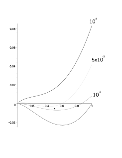
FIG. 4.: Plot of Magnetic charge contribution for different values of the parameter $\alpha_{m}^{2}$. For $\alpha_{m}^{2}=0$, we have the Schwarzschild space.

Even for the magnetic case, we find a behavior of the energy gap similar to the electric one. This means that even in this case, the Casimir energy for RN wormholes is always higher than the Casimir energy for Schwarzschild wormholes.

VI Summary and Conclusions

In this paper we have considered the possibility of forming a foamy spacetime using a collection of $N$ coherent RN wormholes. By applying the same methods used for the Schwarzschild wormholes, we have found that in case of a electric or magnetic potential the Casimir energy is always higher than the one computed for the Schwarzschild case, i.e.

$$\Delta E_{flat}^{RN}\left(M,Q\right)>\Delta E_{flat}^{Schwarzschild}\left(M\right)$$ (98)

. To this purpose to correctly compare such energies the same reference scale has been considered. We would like to remark that for very small electromagnetic field energy contribution, it is the total energy difference between the RN spacetime and flat space which is negative. The single energy contribution of flat space and RN space is strictly positive. Note that this result has been obtained when the number of wormholes is equal to one. Indeed the complete conclusion can be supported when one proofs:

  a)

the existence of an unstable mode;

  b)

a boundary reduction mechanism coming into play in such a way to stabilize the system.

Nevertheless, the purpose of the paper is to proof that the Casimir energy for RN wormholes is always higher than the Schwarzschild Casimir energy. Since this is the case, it is sufficient to assume the validity of point a) and b) to conclude. Note that the result is obtained for every value of $\alpha_{e}^{2}$ and $\alpha_{m}^{2}$ s.t. $0<\begin{array}[]{c}\alpha_{e}^{2}\\ \alpha_{m}^{2}\end{array}<1$. This seems to suggest that a space-time foam formation realized by RN wormholes is suppressed when compared with the foamy space formed by Schwarzschild wormholes. On the other hand one can think to the collection of $N$ RN wormholes as an excited state with respect to the collection of $N$ Schwarzschild wormholes leading to the conclusion that such a collection can be considered as a good candidate for a possible ground state of a quantum theory of the gravitational field, when compared to a superposition of large $N$ RN wormholes.

VII Acknowledgments

I wish to thank J. D. Bekenstein, R. Brout, M. Cavaglià, V. Frolov, C. Kiefer, P. Spindel and C. Vaz for useful comments and discussions.

A Kruskal-Szekeres coordinates for RN spacetime

We have defined the RN line element in Eq.$\left(\ref{p11}\right)$. To introduce the Kruskal-Szekeres[29, 30, 31] type coordinates we consider the following transformation

$\displaystyle ds^{2}=-\left(1-\frac{2MG}{r}+\frac{Q^{2}}{r^{2}}\right)\left[dt^{2}-dr^{\ast 2}\right]+r^{2}d\Omega^{2}$

$$=-\left(1-\frac{2MG}{r}+\frac{Q^{2}}{r^{2}}\right)dvdu+r^{2}\left(u,v\right)d\Omega^{2},$$ (A1)

where $v=t+r^{\ast}$ is the ingoing radial null coordinate and $u=t-r^{\ast}$ is the outgoing radial null coordinate. The “tortoise coordinate” $r^{\ast}$ is defined by

$$dr^{\ast}=\frac{r^{2}dr}{\left(r-r_{-}\right)\left(r-r_{+}\right)}$$ (A2)

$$\Longrightarrow r^{\ast}=r+\frac{1}{2\kappa_{+}}\ln\frac{\left|r-r_{+}\right|}{r_{+}}+\frac{1}{2\kappa_{-}}\ln\frac{\left|r-r_{-}\right|}{r_{-}}+c,$$ (A3)

where $\kappa_{+}$ and $\kappa_{-}$ have been defined by Eq. $\left(\ref{p12ab}\right)$. To avoid singularities we can define Kruskal-Szekeres type coordinates

$$V^{+}=\exp\kappa_{+}v\qquad U^{+}=-\exp-\kappa_{+}u.$$ (A4)

These coordinates do not cover $r\leq r_{-}$ because of the coordinate singularity at $r=r_{-}$ (and $U^{+}V^{+}$ is complex for $r\leq r_{-}$), but $r=r_{-}$ and a similar four regions are covered by the $\left(U^{-},V^{-}\right)$ Kruskal-Szekeres-type coordinates to this case. Thus, let us define

$$V^{-}=\exp\kappa_{-}v\qquad U^{-}=-\exp-\kappa_{-}u.$$ (A5)

For the $+$ sign we have

$$U^{+}V^{+}=-\exp\left(\kappa_{+}\left(v-u\right)\right)=-\exp\left(2\kappa_{+}r^{\ast}\right)=-\exp\left(2\kappa_{+}r\right)\left(\frac{r-r_{+}}{r_{+}}\right)\left(\frac{r-r_{-}}{r_{-}}\right)^{\frac{\kappa_{+}}{\kappa-}}$$ (A6)

and the respective line element is

$$ds_{+}^{2}=-\frac{r_{+}r_{-}}{\kappa_{+}^{2}}\frac{\exp\left(-2\kappa_{+}r\right)}{r^{2}}\left(\frac{r_{-}}{r-r_{-}}\right)^{\frac{\kappa_{+}}{\kappa-}-1}dU^{+}dV^{+}+r^{2}\left(U^{+},V^{+}\right)d\Omega^{2},$$ (A7)

while for the $-$ sign we have

$$U^{-}V^{-}=-\exp\left(\kappa_{-}\left(v-u\right)\right)=-\exp\left(2\kappa_{-}r^{\ast}\right)=-\exp\left(2\kappa_{-}r\right)\left(\frac{r_{-}-r}{r_{-}}\right)\left(\frac{r_{+}-r}{r_{+}}\right)^{\frac{\kappa_{-}}{\kappa_{+}}}$$ (A8)

and the associated line element is

$$ds_{-}^{2}=-\frac{r_{+}r_{-}}{\kappa_{-}^{2}}\frac{\exp\left(-2\kappa_{-}r\right)}{r^{2}}\left(\frac{r_{+}}{r_{+}-r}\right)^{\frac{\kappa_{-}}{\kappa_{+}}-1}dU^{-}dV^{-}+r^{2}\left(U^{-},V^{-}\right)d\Omega^{2}.$$ (A9)

The conformal Penrose diagram of the RN space is shown in Fig.2.

B The Hamiltonian contribution of the Electromagnetic field

The form of the hamiltonian for the electromagnetic field can be obtained with the same method used for the pure gravitational field. Let $u_{\alpha}$ a normalized time-like vector field s.t. $u_{\alpha}u^{\alpha}=-1$. The form of ${\cal H}_{M}$ comes from the Einstein-Maxwell action and it can be written as

$${\cal H}_{M}=\sqrt{{}^{3}g}T_{\alpha\beta}u^{\alpha}u^{\beta},$$ (B1)

where

$$T_{\alpha\beta}=\frac{1}{4\pi}\left[F_{\alpha\gamma}F_{\beta}^{\gamma}-\frac{1}{4}g_{\alpha\beta}F_{\gamma\delta}F^{\gamma\delta}\right]$$ (B2)

and $F_{\alpha\gamma}=\partial_{\alpha}A_{\gamma}-\partial_{\gamma}A_{\alpha}$. $A_{\alpha}$ is the electromagnetic potential which, in the case of a pure electric field assumes the form $A_{\alpha}=\left(Q_{e}/r,0,0,0\right)$ while in the case of pure magnetic field, the form is $A_{\alpha}=\left(0,-Q_{m}\sin\theta,0,0\right)$. $Q_{e}$ and $Q_{m}$ are the electric and magnetic charge respectively. Both of them contribute in the same way to the gravitational potential of Eq. $\left(\ref{p12}\right)$. Since we are interested in electric type R.N. metrics, the on-shell contribution of $T_{\alpha\beta}u^{\alpha}u^{\beta}$ is

$$T_{\alpha\beta}u^{\alpha}u^{\beta}=\frac{1}{8\pi}\left(F_{01}\right)^{2}=\frac{1}{8\pi}\frac{Q_{e}^{2}}{r^{4}}.$$ (B3)

Nevertheless, this is not the complete contribution when gravitational fluctuations come into play. Indeed up to second order in $h_{ij}$, one gets

$$\int_{\Sigma}d^{3}x{\cal H}_{M}=2\kappa\int_{\Sigma}d^{3}x\sqrt{{}^{3}\bar{g}}\left[-\frac{1}{4}h_{ij}h^{ij}\left(T_{\alpha\beta}u^{\alpha}u^{\beta}\right)+T_{\alpha\beta}^{\left(2\right)}u^{\alpha}u^{\beta}\right],$$ (B4)

where $T_{\alpha\beta}^{\left(2\right)}u^{\alpha}u^{\beta}=\frac{1}{8\pi}\left(F_{01}\right)^{2}h_{1}^{1}h_{1}^{1}$. Thus Eq. $\left(\ref{app22}\right)$ becomes

$$\int_{\Sigma}d^{3}x{\cal H}_{M}=-\frac{2\kappa}{8\pi}\int_{\Sigma}d^{3}x\sqrt{{}^{3}\bar{g}}\left[-\frac{3}{4}h_{1}^{1}h_{1}^{1}\left(F_{01}\right)^{2}+\frac{1}{4}h_{2}^{2}h_{2}^{2}\left(F_{01}\right)^{2}+\frac{1}{4}h_{3}^{3}h_{3}^{3}\left(F_{01}\right)^{2}\right].$$ (B5)

On the other hand, when we consider the magnetic charge, the on-shell contribution of $T_{\alpha\beta}u^{\alpha}u^{\beta}$ is

$$T_{\alpha\beta}u^{\alpha}u^{\beta}=\frac{1}{8\pi}\left(F_{23}\right)^{2}=\frac{1}{8\pi}\frac{Q_{m}^{2}}{r^{4}}.$$ (B6)

However for the magnetic part, one gets

$$T_{\alpha\beta}u^{\alpha}u^{\beta}\varpropto F_{ij}F^{ij}=F_{ij}F_{kl}g^{ik}g^{jl}$$ (B7)

then to second order in $h_{ij}$ one obtains

$$\int_{\Sigma}d^{3}x{\cal H}_{M}=-\frac{2\kappa}{16\pi}\int_{\Sigma}d^{3}x\sqrt{{}^{3}\bar{g}}\left[\frac{1}{4}h_{1}^{1}h_{1}^{1}\left(F_{23}\right)^{2}-\frac{7}{4}h_{2}^{2}h_{2}^{2}\left(F_{23}\right)^{2}-\frac{7}{4}h_{3}^{3}h_{3}^{3}\left(F_{23}\right)^{2}\right].$$ (B8)

C Action and Hamiltonian

Here we follow Ref.[17] to extract the form of the Hamiltonian in presence of a bifurcation surface with boundaries. We will consider for simplicity the case of a single horizon, like the Schwarzschild one, the generalization for the Reissner-Nordström case is straightforward. We consider two spacelike Cauchy surfaces $\Sigma^{\prime}$ and $\Sigma^{\prime\prime}$. The region lying between $\Sigma^{\prime}$ and $\Sigma^{\prime\prime}$ consists of two wedges $M_{+}$ and $M_{-}$ intersecting at a two-dimensional surface $S_{0}$. The symbol $\Sigma_{t\,(\pm)}$ denotes the part of $\Sigma_{t}$ located in $M_{\pm}$. We also denote those parts of $\Sigma^{\prime}$ and $\Sigma^{\prime\prime}$ which are the spacelike boundaries of the wedges $M_{\pm}$ as $\Sigma_{\pm}^{\prime}$ and $\Sigma_{\pm}^{\prime\prime}$. The lapse function $N$ is positive (negative) at $M_{+}$ ($M_{-}$) and equals zero at the bifurcation surface. The vector $u^{\mu}=-N\partial_{\mu}t$ is future oriented in $M_{+}$ and past oriented in $M_{-}$. The metric is described in Eq.$\left(\ref{p14}\right)$ and the covariant form of the gravitational action for this foliation with fixed three-geometry at the boundaries of $M$ is

$\displaystyle S={\frac{1}{2\kappa}}\int_{M_{+}}d^{4}x\,\sqrt{-g}\,\Re+{\frac{1}{\kappa}}\int_{t^{\prime}({+})}^{t^{\prime\prime}}d^{3}x\,\sqrt{g^{\left(3\right)}}\,K-{\frac{1}{\kappa}}\int_{{B_{+}}}d^{3}x\,\sqrt{-\gamma}\,\Theta-S_{0\left(+\right)}$

$$-{\frac{1}{2\kappa}}\int_{M_{-}}d^{4}x\,\sqrt{-g}\,\Re+{\frac{1}{\kappa}}\int_{t^{\prime}({-})}^{t^{\prime\prime}}d^{3}x\,\sqrt{g^{\left(3\right)}}\,K-{\frac{1}{\kappa}}\int_{{B}_{-}}d^{3}x\,\sqrt{-\gamma}\,\Theta\ -S_{0\left(-\right)}.$$ (C1)

$\Re$ denotes the four-dimensional scalar curvature, $\kappa\equiv 8\pi G$, and

$\displaystyle\sqrt{-g}=|N|\sqrt{h}$

$$\sqrt{-{\gamma}}=|N|\sqrt{\sigma},$$ (C2)

where $\sigma$ is the determinant of the two-dimensional metric $\sigma_{ab}$. $K$ is the extrinsic curvature of $\Sigma_{t}$ as a surface embedded in $M$, while $k$ is the extrinsic curvature of the boundaries $S$ embedded on $\Sigma$. Then the trace of the extrinsic curvature of the boundaries $B$ as surfaces embedded in $M$ is

$$\Theta=k-n_{\beta}a^{\beta}\ ,$$ (C3)

where $a^{\mu}=u^{\alpha}\nabla_{\alpha}u^{\mu}$ is the acceleration of the timelike normal $u^{\mu}$. $B$ is a three-dimensional timelike boundary such that $B=B_{+}\cup B_{-}$. The spacelike normal $n^{i}$ to the three-dimensional boundaries $B$ is assumed to be outward pointing at $B_{+}$, inward pointing at $B_{-}$. It is assumed that the integrations are taken over the coordinates $x^{\mu}$ which have the same orientation as the canonical coordinates $(t,x,\theta,\phi)$ of the foliation. The negative sign for the integration over $M_{-}$ reflects the fact that the canonical coordinates are left oriented in this region. Besides the volume term, the action $S$ contains also boundary terms. The notation $\int_{t^{\prime}({\pm})}^{t^{\prime\prime}}$ represents an integral over the three-boundary $\Sigma_{\pm}$ at $t^{\prime\prime}$ minus an integral over the three-boundary $\Sigma_{\pm}$ at $t^{\prime}$. Under a $3+1$ spacetime split, the four-dimensional scalar curvature is

$$\Re=R^{\left(3\right)}+K_{\mu\nu}K^{\mu\nu}-(K)^{2}-2\nabla_{\mu}(Ku^{\mu}+a^{\mu})\ ,$$ (C4)

where $R$ denotes the scalar curvature of the three-dimensional spacelike hypersurface $\Sigma$. By the use of Gauss’ theorem, the conditions

$$u\cdot n|_{B}=0,\,u\cdot a=0,\,u\cdot u=-1,\,n\cdot n=1\ ,$$ (C5)

and Eqns. (C1)-(C3) and (C4), one can rewrite the total action in the form

$\displaystyle S={\frac{1}{2\kappa}}\int_{M_{+}}d^{4}x\sqrt{-g}\,\left[R+K_{\mu\nu}K^{\mu\nu}-(K)^{2}\right]-{\frac{1}{\kappa}}\int_{{B_{+}}}d^{3}x\sqrt{-\gamma}\,k$

$$-{\frac{1}{2\kappa}}\int_{M_{-}}d^{4}x\sqrt{-g}\,\left[R+K_{\mu\nu}K^{\mu\nu}-(K)^{2}\right]-{\frac{1}{\kappa}}\int_{{B_{-}}}d^{3}x\sqrt{-\gamma}\,k\ .$$ (C6)

The action for stationary solutions finally becomes

$$S=-\int Hdt\ ,$$ (C7)

with the gravitational Hamiltonian $H$ given by

$$H=\int_{\Sigma}d^{3}x\left(N{\cal H}+N^{i}{{\cal H}_{i}}\right)+\frac{1}{\kappa}\int_{{S_{+}}}d^{2}x\sqrt{\sigma}Nk-\frac{1}{\kappa}\int_{{S_{-}}}d^{2}x\sqrt{\sigma}Nk.$$ (C8)

REFERENCES

- [1] S. Coleman, Nucl. Phys. B 298 (1988), 178; S. Coleman, Aspects of Symmetry (Cambridge University Press, Cambridge, 1985).
- [2] R. Bousso and S.W. Hawking, Phys. Rev. D 52, 5659 (1995), gr-qc/9506047; R. Bousso and S.W. Hawking, Phys. Rev. D 54, 5659 (1995), gr-qc/9606052.
- [3] D.J. Gross, M.J. Perry and L.G. Yaffe, Phys. Rev. D 25, (1982) 330.
- [4] P. Ginsparg and M.J. Perry, Nucl. Phys. B 222 (1983) 245.
- [5] R.E. Young, Phys. Rev. D 28, (1983) 2436; R.E. Young, Phys. Rev. D 28 (1983) 2420.
- [6] M.S. Volkov and A. Wipf, Nucl.Phys.B 582 (2000), 313; hep-th/0003081.
- [7] T. Prestidge, Phys.Rev. D 61 (2000) 084002, hep-th/9907163.
- [8] P.K. Townsend, Black Holes: Lectures Notes, gr-qc/9707012.
- [9] R.Garattini, Int. J. Mod. Phys. A 18 (1999) 2905, gr-qc/9805096.
- [10] R. Garattini, Phys. Lett. B 446 (1999) 135, hep-th/9811187.
- [11] R. Garattini, Phys. Lett. B 459 (1999) 461, hep-th/9906074.
- [12] R. Garattini, A Spacetime Foam approach to the cosmological constant and entropy. To appear in Int.J.Mod.Phys. D; gr-qc/0003090.
- [13] R. Garattini, Nucl.Phys.Proc.Suppl. 88 (2000) 297. gr-qc/9910037.
- [14] R. Garattini, Class.Quant.Grav. 17 (2000) 3335, gr-qc/0006076.
- [15] R. Garattini, Int. J. Mod. Phys. A 18 (1999) 2905, gr-qc/9805096.
- [16] R. Garattini, Phys.Rev. D 59 (1999) 104019, hep-th/9902006.
- [17] V.P. Frolov and E.A. Martinez, Class.Quant.Grav.13 :481-496,1996, gr-qc/9411001.
- [18] S. W. Hawking and G. T. Horowitz, Class. Quant. Grav. 13 1487, (1996), gr-qc/9501014.
- [19] I. Radinschi, Energy Distribution of a Charged regular Black Hole, gr-qc/0011066.
- [20] J. M. Cornwall, R. Jackiw and E. Tomboulis, Phys. Rev. D 8, 2428 (1974).
- [21] M. Consoli and G. Preparata, Phys. Lett. B, 154, 411 (1985).
- [22] M. Berger and D. Ebin, J. Diff. Geom. 3, 379 (1969).
- [23] J. W. York Jr., J. Math. Phys., 14, 4 (1973); J. W. York Jr., Ann. Inst. Henri Poincaré A21, 319 (1974).
- [24] P. A. Griffin and D. A. Kosower, Phys. Lett. B 233, 295 (1989).
- [25] G. Esposito, A. Yu Kamenshchik and G. Pollifrone, Euclidean Quantum Gravity on Manifolds with Boundary. Fundamental Theories of Physics, vol 85 (Dordrecht: Kluwer, 1997).
- [26] T. Regge and J. A. Wheeler, Phys. Rev. 108, 1063 (1957).
- [27] S.A. Ridgway and E.J. Weinberg, Phys.Rev.D 51 (1995), 638; hep-th/9409013.
- [28] S.S. Gubser and I. Mitra, Instability of charged black holes in anti-de Sitter space, hep-th/0009126.
- [29] M.D. Kruskal, Phys. Rev. 119, (1960) 1743; G. Szekeres, Publ. Math. Debreceni 7 (1960) 285.
- [30] S.W. Hawking and G.F.R. Ellis, The Large Scale Structure of Spacetime (Cambridge Univ. Press, 1973).
- [31] C.W. Misner, K.S. Thorne and J.A. Wheeler, Gravitation (Freeman, San Francisco, 1973) 842.