A causally connected superluminal Warp Drive spacetime

Abstract

It will be shown that while horizons do not exist for warp drive spacetimes traveling at subluminal velocities horizons begin to develop when a warp drive spacetime reaches luminal velocities. However it will be shown that the control region of a warp drive ship lie within the portion of the warped region that is still causally connected to the ship even at superluminal velocities, therefore allowing a ship to slow to subluminal velocities. Further it is shown that the warped regions which are causally disconnected from a warp ship have no correlation to the ship velocity.

1 Introduction

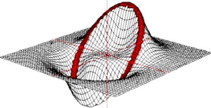
Figure 2: Luminal horizon formation. The red region represents where a horizon will form once a warp drive spacetime [1] reaches lumnial velocities.

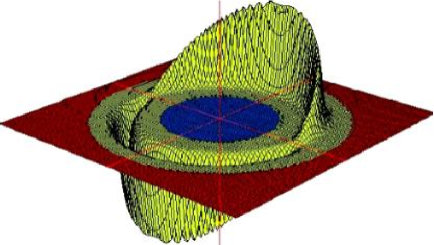
Figure 3: Superluminal warp bubble frame regions. The blue region is the remote frame horizon, the yellow region is the Pfenning region, and the red region is the ship frame horizon.

One of the many obstacles posed by rightfully skeptical physicists against the warp drive is the appearance of horizons when a ship travels at superluminal velocities (see figure 2). This is a problem, to control the speed of the ship because if the bubble becomes causally disconnected from the ship then observers in the ship frame cannot turn off the bubble so the ship cannot reduce its velocity. If the ship becomes causally disconnected from the bubble then possible voyages to Messier–42 Orion nebula at 1500 light-years from Earth or Messier–1 at 6000 light years from Earth would be impossible because the ship being causally disconnected from the bubble cannot turn off the bubble and cannot reach its destination. If a ship is causally disconnected from the bubble then the warp drive must be turned off from outside the ship’s frame and we don’t know if there is “someone out there” at Orion or Crab to turn off the run away warp bubble. In this work we show that while part of the warped region becomes causally disconnected from a ship when the ship is luminal or superluminal the behaviour of that part does not depend on the ship speed and can be engineered while the ship is still subluminal. Also it shown the control region of the ship’s velocity remains in the portion of the warped region that is still casually connected to the ship (see figure 3).

2 two-dimensional warp drive

In order to explore the superluminal control problem of the warp drive we now set up the mathematics which define the physical horizons (the red region of figure 2). In order to do so it will be necessary to write a two dimensional ESAA metric [1] written in the Alcubierre formalism:

$$ds^{2}=-A^{2}dt^{2}+[dx-v_{s}f(r_{s})dt]^{2}$$ (1)

where

$$dx=dx^{\prime}+v_{s}dt$$

$$v_{s}={dx_{s}\over dt}$$

requiring that

$$ds^{2}=-A^{2}dt^{2}+[dx^{\prime}+v_{s}dt-v_{s}f(r_{s})dt]^{2}$$ (2)

where we can replace with

$$ds^{2}=-A^{2}dt^{2}+[dx^{\prime}+v_{s}dt(1-f(r_{s}))]^{2}$$ (3)

for simplicity we write

$$1-f(r_{s})={\cal S}(r_{s}).$$

So that we arrive at:

$$ds^{2}=-A^{2}dt^{2}+dx^{\prime 2}+2v_{s}{\cal S}(r_{s})dx^{\prime}dt+(v_{s}{\cal S}(r_{s}))^{2}dt^{2}$$ (4)

which leads to

$$ds^{2}=A^{2}dt^{2}-(v_{s}{\cal S}(r_{s}))^{2}dt^{2}-2v_{s}{\cal S}(r_{s})dx^{\prime}dt-dx^{\prime 2}$$ (5)

or

$$ds^{2}=[A^{2}-(v_{s}{\cal S}(r_{s}))^{2}]dt^{2}-2v_{s}{\cal S}(r_{s})dx^{\prime}dt-dx^{\prime 2}$$ (6)

thereby arriving at a two-dimensional ESAA spacetime necessary to discuss the mathematics behind the ‘horizon problem,’ and how to overcome it.

2.1 Two-dimensional ESAA Hiscock Horizons

In order to discuss the ‘horizon problem’ we will be improving upon the paradigm set forth by Hiscock [2]. Such that an ESAA-Hiscock ship frame metric can be written from:

$$ds^{2}=-H(r_{s})dT^{2}+{A^{2}(r_{s})dx^{\prime 2}\over H(r_{s})}$$ (7)

with

$$dT=dt-{v_{s}{\cal S}(r_{s})\over H(r_{s})}dx^{\prime}$$ (8)

such that we can receive

$$ds^{2}= -H(r_{s})dt^{2}-2v_{s}{\cal S}(r_{s})dx^{\prime}dt/H(r_{s})$$ (9)

$$+(v_{s}{\cal S}(r_{s})/H(r_{s}))^{2}dx^{\prime 2}+A^{2}(r_{s})dx^{\prime 2}/H(r_{s})$$

by choosing

$$H(r_{s})=A^{2}-(v_{s}{\cal S}(r_{s}))^{2}$$ (10)

we have a horizon function. We can thus have the corresponding line element

$$ds^{2}= -H(r_{s})dt^{2}+2v_{s}{\cal S}(r_{s})dx^{\prime}dt-A^{2}dx^{\prime 2}/H(r_{s})$$ (11)

$$+H(r_{s})dx^{\prime 2}/H(r_{s})+A^{2}dx^{\prime 2}/H(r_{s})$$

which reduces to

$$ds^{2}=-H(r_{s})dt^{2}+2v_{s}{\cal S}(r_{s})dx^{\prime}dt+dx^{\prime 2}$$ (12)

or

$$ds^{2}=-[A^{2}-(v_{s}{\cal S}(r_{s}))^{2}]dt^{2}+2v_{s}{\cal S}(r_{s})dx^{\prime}dt+dx^{\prime 2}$$ (13)

3 Pfenning piecewise function in terms of A

Starting with an arbitrary two-dimensional horizon (10) we can now begin to define the value of $A$. In the Pfenning integration limits $R-(\Delta/2)$ and $R+(\Delta/2)$ [3], whereby we set $\Delta=2/\sigma$ and $\sigma=14$ from the Alcubierre top hat function

$$f(r_{s})={\tanh[\sigma(r_{s}+R)]-\tanh[\sigma(r_{s}-R)]\over 2\tanh(\sigma R)}.$$

By the Pfenning limits the values for the lapse function becomes

$$A(r_{s})=\left\{{\begin{array}[]{*{20}c}1&{r_{s}<R-(\Delta/2)}\\ {\kappa_{L}}&{R-(\Delta/2)\leq r_{s}\leq R+(\Delta/2)}\\ 1&{r_{s}>R+(\Delta/2)}\\ \end{array}}\right.$$ (14)

Where $\kappa_{L}$ is a large constant, we also note that A can not be a function of the speed. We now wish to introduce the values of the Pfenning Piecewise function $f(r_{s})$.

$$f(r_{s})=\left\{{\begin{array}[]{*{20}c}1&{r_{s}<R-(\Delta/2)}\\ {1-(1/A)r_{s}-R}&{R-(\Delta/2)\leq r_{s}\leq R+(\Delta/2)}\\ 0&{r_{s}>R+(\Delta/2)}\\ \end{array}}\right.$$ (15)

and now the ESAA ship frame Piecewise function ${\cal S}(r_{s})$

$${\cal S}(r_{s})=\left\{{\begin{array}[]{*{20}c}0&{r_{s}<R-(\Delta/2)}\\ {(1/A)r_{s}+R}&{R-(\Delta/2)\leq r_{s}\leq R+(\Delta/2)}\\ 1&{r_{s}>R+(\Delta/2)}\\ \end{array}}\right.$$ (16)

The Pfenning Piecewise and ESAA Piecewise functions are defined in function of the term A. This will have some advantages that will be shown in the work -we will study now the behaviour of the ESAA-Hiscock Horizon function in three situations:

• 1-ship subluminal ($v<1$)

• 2-ship luminal ($v=1$)

• 3-ship superluminal ($v>1$)

We do so by defining the ESAA-Hiscock horizon (10) with the following function

$$H(r_{s})=\left\{{\begin{array}[]{*{20}c}1&{r_{s}<R-(\Delta/2)}&{H(r_{s})>0}\\ {A^{2}-(v_{s}/A)^{2}}&{r_{s}=R-(\Delta/2)}&{H(r_{s})>0}\\ {A^{2}}&{r_{s}=R}&{H(r_{s})>0}\\ {A^{2}-(v_{s}/A)^{2}}&{r_{s}=R+(\Delta/2)}&{H(r_{s})>0}\\ {A^{2}-{(v_{s}/A)(r_{s}-R)}^{2}}&{R-(\Delta/2)<r_{s}<R+(\Delta/2)}\\ \end{array}}\right.$$ (17)

3.1 subluminal ship velocities

It is clear why there are no horizons for the proposed spacetime (13) with the functions (14,15,16,17). Since in this case one is left with the general definition $H(r_{s})>0$. Since A is large from the above expressions it can be seen that the ESAA-Hiscock Horizon function never drops to zero. It is also noted that A is not function of the speed and A is included in the definition of the Piecewise continuous functions that warrants for large A the ship will be always connected to the region from $r_{s}=0$ (ship location) to $r_{s}=R+(\Delta/2)$ (upper Pfenning limit). Since we have $A=1$ and ${\cal S}(r_{s})=1$ for $r_{s}>R+(\Delta/2)$ we obtain

$$H(r_{s})=1-v_{s}^{2}H(r_{s})>0$$

telling us that subluminal warp shells are causally connected to the ship. In this region A must drop back from a large value at $r_{s}=R+(\Delta/2)$ to $A=1$ at $r_{s}>R+(\Delta/2)$ then part of the warped region is beyond $R+(\Delta/2)$ since we need exotic matter to force the A back to 1. Furthermore since A is not function of the speed if the ship changes its speed the behaviour of A will not be affected. Since $H(r_{s})>0$ the ship is causally connected to this region and is therefore subluminal.

3.2 luminal ship velocities

From the functions (14,16,17) we can now again set up the general definition $H(r_{s})>0$. Since $A$ is large from the above expressions it can be seen that the ESAA-Hiscock Horizon function never drops to zero. Again $A$ is not a function of the speed and $A$ is included in the definition of the Piecewise functions that warrants for large A the ship will be always connected to the region from $r_{s}=0$ (ship location) to $r_{s}=R+(\Delta/2)$ (upper Pfenning limit). $H(r_{s})=0$ since $A=1$ and ${\cal S}(r_{s})=1$ and $v_{s}=1$, $r_{s}>R+(\Delta/2)$, thus from eq. (7), we see that a horizon will appear at luminal speeds the ship becomes causally disconnected from the region beyond $R+(\Delta/2)$. Since A is large at $r_{s}=R+(\Delta/2)$ and must drop back to 1 when $r_{s}>R+(\Delta/2)$ we still need exotic matter beyond $R+(\Delta/2)$ to drop the value of A back to 1 and this warped region is causally disconnected from the ship, the ship remains causal until $r_{s}=R+(\Delta/2)$. Providing that A is not function of the speed then A is not affected when the horizon appears in front of the ship when the ship gets luminal, the behaviour of A was engineered when the ship was subluminal. And the part of the speed control still lies in the region between $\int_{R-(\Delta/2)}^{R+(\Delta/2)}r_{s}$ so the ship can change the speed and go back to subluminal if needed.

3.3 superluminal ship velocities

Finally the for the superluminal warp drive we again have the following definition $H(r_{s})>0$. Since A is large from the above expressions it can be seen that the ESAA-Hiscock Horizon function never drops to zero A is not function of the speed and A is included in the definition of the Piecewise functions that warrants for large A the ship will be always connected to the region from $r_{s}=0$ (ship location) to $r_{s}=R+(\Delta/2)$ (upper Pfenning limit). $H(r_{s})<0$ since $A=1$ and ${\cal S}(r_{s})=1$ and $v_{s}>1$ $r_{s}>R+(\Delta/2)$, again from eq. (7) we see that a horizon will appear. At superluminal speeds the ship becomes causally disconnected from the region beyond $R+(\Delta/2)$. Assuming a continuous spacetime (Alcubierre) $H(r_{s})>0$ at $r_{s}=R+(\Delta/2)$ but $H(r_{s})<$ 0 at $r_{s}>R+(\Delta/2)$, somewhere between $H(r_{s})=0$ and then we have the horizon. Since A is large at $r_{s}=R+(\Delta/2)$ and must reduce to 1 when $r_{s}>R+(\Delta/2)$ we still need exotic matter beyond $R+(\Delta/2)$ to lower the value of A back to 1 and this warped region is causally disconnected from the ship which remains causal until $r_{s}=R+(\Delta/2)$. Providing that A is not function of the speed then A is not affected when the Horizon appears in front of the ship when the ship goes superluminal. The behaviour of A was engineered when the ship was subluminal and the part of the speed control still lies in the region between $\int_{R-(\Delta/2)}^{R+(\Delta/2)}r_{s}$ so the ship can change the speed and go back to subluminal if needed.

4 energy momentum tensor

Consider now the following stress energy momentum tensor for a ship frame ESAA-warp metric

$$T^{00}=-\frac{v_{s}^{2}}{4}{1\over 8\pi}\left({d{\cal S}(r_{s})\over dr_{s}}\right)^{2}\left({\sigma\over r_{s}}\right)^{2}\frac{1}{A^{4}}$$ (18)

defining $d{\cal S}(r_{s})/dr_{s}=1/A$, implies that

$$T^{00}=-{v_{s}^{2}\over 4}{1\over 8\pi}\left({\sigma\over r_{s}}\right)^{2}\frac{1}{A^{6}}$$ (19)

which has the capacity to lower the negative energy densities of a warp drive spacetime even further.

5 on colliding warp shells

The remote frame ESAA warp drive metric is given by:

$$ds^{2}=-A^{2}dt^{2}+[dx-v_{s}f(r_{s})dt]^{2}$$ (20)

with $A=1$ inside and outside the ship frame and in the warped region comes to some large value $k_{l}$. The function $f(r_{s})$ has the ordinary values for top hat functions except at:

$$f(r_{s})=1-(1/A)(r_{s}-R)\iff R-(\Delta/2)\leq r_{s}\leq R+(\Delta/2)$$

for calculating horizons we are concerned with the region $g_{00}=[A^{2}-(v_{s}f(r_{s}))^{2}]$, so we will examine the behaviour of $g_{00}$ with $v_{s}r_{s}<R+(\Delta/2)$

$$g_{00}=1-v_{s}^{2}\iff v_{s}<1$$ (21)

this is causally connected to the remote frame, while $v_{s}\geq 1$ is disconnected from the remote frame, only with the conditions $v_{s}<1\leftrightarrow g_{00}>0$ do horizons fail appear. Another way to remove the horizons is to modify the space such that

$$g_{00}=A^{2}-(v_{s}[1-(1/A)(r_{s}+R)])^{2}$$ (22)

thus providing a large constant value for A, $g_{00}>0$ thus this region becomes causally connected to the remote frame.

As seen from remote observer in flat spacetime $g_{00}=1$, thus when the ship is superluminal the horizon lies at $r_{s}>R+(\Delta/2)$. From the ship frame this forms the ship horizon, the ship is causally connected from the region $r_{s}=0$ to $r_{s}=R+(\Delta/2)$ When the ship is superluminal the horizon lies at $r_{s}<R-(\Delta/2)$ for a remote frame observer, this is the remote frame horizon. The remote frame is causally connected from $r_{s}>R+(\Delta/2)$ at a great distance and remains connected until $r_{s}=R-(\Delta/2)$ the ship frame cannot send signals to $r_{s}>R+(\Delta/2)$ the remote frame cannot send signals to $r_{s}<R-(\Delta/2)$ but the region between $\int_{R-(\Delta/2)}^{R+(\Delta/2)}r_{s}$ remains connected to both observers if an astronaut changes the speed the outer parts of the bubble will react although the astronaut cannot communicate with the outer parts of the bubble, thus if the region between $\int_{R-(\Delta/2)}^{R+(\Delta/2)}r_{s}$ is common to both observers the bubble will not collapse.

5.1 Preprogrammed A

Although we set up to define A by ”pre-programmed exotic matter” which does not change when the ship pass from subluminal to superluminal velocity (see figure 3), we have not defined $k_{l}$. For a Pfenning Piecewise behaviour of A in the upper Pfenning limit $R+(\Delta/2)$, $A$ still have a large value to keep this part causally connected to the ship according to ESAA-Hiscock function (10) by making $H(r_{s})>0$ even when $v_{s}>1$. Then we have the following values for $A$ according to $r_{s}$ (already seen from eq. (17)). Providing that $A$ is not function of the speed the ship will be disconnected after $r_{s}>R+(\Delta/2)$ but this does not affect the behaviour of $A$. The Pfenning piecewise function is an approximation used first by Pfenning to simplify calculations and we are adopting Pfenning techniques here. We know that the continuous form of the top hat $f(r_{s})$ is 1 in the ship and 0 far from it, there exists a open interval $\int_{0}^{1}f(r_{s})$ when the function $f(r_{s})$ starts to decrease from 1 to 0. It is in that region where the exotic matter resides which is the continuous equivalent of the Pfenning warped region.

If we define

$$A={1\over 2}\left(1+\tanh[\sigma(r_{s}-R)^{2}]\right)^{-N}$$ (23)

where $-N$ is an arbitrary exponent designed to reduce stress-energy requirements. We will have a continuous form of $A$ defined in function of the continuous Alcubierre top hat $f(r_{s})$ and $A$ is function of $r_{s},R,\sigma$ and $N$. This expression can make $A$ be 1 in the ship and far from it while being large in the warped region…the region where $f(r_{s})$ starts to decrease from 1 to 0.

Below there are numerical evaluations (see table 1) showing the behaviour of $A$ reducing to 1 after the warped region even if the ship is disconnected due to function of distance $r_{s}$. And therefore “pushing” the ESAA-Hisccock horizon to the outermost layers of the warped region making the speed controllable by the ship because the major part of the warped region is connected to the ship so the ship can reduce to subluminal velocities.

Table 1: Warp shell numerical evaluations.

$r_{s}$	$R$	$\sigma$	$f(r_{s})$	$S(r_{s})$	$A$
0	50	0.1	1	0	1.023
10	50	0.1	0.9997	0.0002	1.1825
20	50	0.1	0.9997	0.0023	3.4228
30	50	0.1	0.9997	0.0178	8031
40	50	0.1	0.9976	0.1191	$3.0\times 10^{25}$
50	50	0.1	0.5	0.5	$2\times 10^{75}$
60	50	0.1	0.1192	0.8807	$3.9\times 10^{25}$
70	50	0.1	0.0179	0.9820	$4.16\times 10^{15}$
80	50	0.1	0.0024	0.9975	140.5
90	50	0.1	0.0003	0.9976	1.9956
100	50	0.1	$4.5\times 10^{-5}$	0.9999	1.0950

5.2 remote frame

We now introduce a Hiscock horizon function for the remote frame

$$I(r_{s})=A^{2}-(v_{s}f(r_{s}))^{2}$$ (24)

therefore the line element of remote frame observer is

$$ds^{2}=-I(r_{s})dT^{2}+{A^{2}\over I(r_{s})}\;dx^{2}$$ (25)

lending

$$dT^{2}=dt^{2}+{2v_{s}f(r_{s})dxdt\over I(r_{s})}+\left({v_{s}f(r_{s})\over I(r_{s})}\right)^{2}dx^{2}$$ (26)

recalling that $(v_{s}f(r_{s}))^{2}=A^{2}-I(r_{s})$ yields

$$dT^{2}=dt^{2}+{2v_{s}f(r_{s})dxdt\over I(r_{s})}+{A^{2}-I(r_{s})\over I(r_{s})^{2}}dx^{2}$$ (27)

which reduces to

$$ds^{2}=I(rs)dt^{2}+2v_{s}f(r_{s})dxdt-dx^{2}$$ (28)

from the definition $I(r_{s})=A^{2}-(v_{s}f(r_{s}))^{2}$ we have the following spacetime:

$$ds^{2}=[A^{2}-(v_{s}f(r_{s}))^{2}]dt^{2}+2v_{s}f(r_{s})dxdt-dx^{2}$$ (29)

then we recovered the ESAA remote frame metric from a equivalent ESAA Hiscock Horizon function for the remote frame. Thus a remote frame observer would be given from

$$ds^{2}=-I(r_{s})dT^{2}+{A^{2}\over I(r_{s})}\;dx^{2}$$ (30)

If $v_{s}<1\leftrightarrow I(r_{s})>0$ then the region is causally connected to ship and remote frame. However if $v_{s}=1\leftrightarrow I(r_{s})=0$ the horizon appears for the remote frame, this region while connected to the ship frame becomes causally disconnected from the remote frame, if $v_{s}>1\leftrightarrow I(r_{s})<0$ and assuming a continuous spacetime $I(r_{s})<0$ at $r_{s}<R-(\Delta/2)$ between $R-(\Delta/2)\leq r_{s}\leq R+(\Delta/2)I(r_{s})>0$ then somewhere between $R-(\Delta/2)$ and $r_{s}<R-(\Delta/2)$ a horizon appears which is causally disconnected from the remote frame while connected to the ship frame.

Figure 1: Superluminal Warp Drive with control maintained with inner and outer warp shells defined by $A=(1+\tanh[\sigma(r_{s}+R)]^{2})/2$, which simulates figure 3. Graphed with the following parameters $v_{s}=1$, $\sigma=2$, and $R=1.8$, $\Delta=0.1$ for the flat outer Pfenning region.

If we utilize the top hat function (15) for the warped region $R-(\Delta/2)\leq r_{s}\leq R+(\Delta/2)$ then one has

$$I(r_{s})=A^{2}-v({\cal W})$$ (31)

with

$$v({\cal W})=\sqrt{1-{v_{s}^{2}(r_{s}-R)^{2}\over A(ct,r_{s})^{2}}}$$ (32)

and providing a large $A^{2}>>{v_{s}f(r_{s})}^{2}$ then $I(r_{s})>0$ and this region will be causally connected to the remote frame. The remote frame “sees” the Pfenning warped region (the part of the warped region responsible for the speed), thus the remote frame is causally connected to this region. If an astronaut changes the speed because the astronaut is causally connected to this region then the remote frame will “see” the changing speed. For $I(r_{s})=1$ this part of the warped region is always connected to the remote frame as this part of the warped region must make A drop back to 1 again this region is connected to the remote frame observer and is disconnected from the ship frame while luminal or superluminal.

Thus a signal sent by the ship can go to $r_{s}=R+(\Delta/2)$ and a signal sent by remote observer can go to $r_{s}=R-(\Delta/2)$. Therefore the region between $R-(\Delta/2)\leq r_{s}\leq R+(\Delta/2)$ is “seen” by both observers ship and remote frame. Since the ship “sees” $H(r_{s})$ the remote ”sees” $I(r_{s})$ therefore an astronaut can change the ship speed because this region is connected to the ship the remote frame ”sees” the speed being changed because this region is connected to the remote frame.

So the outer part of the bubble “suffers” when the speed is changed although the astronaut cannot communicate with the outer parts of the bubble and the remote observer cannot communicate with the inner part of the bubble, thus the bubble remains stable for these regions.

6 Conclusion

In this work it was demonstrated how an $A$ defined as a Pfenning-Piecewise like style function can resolve the superluminal control problem of the warp drive. It is assumed that A do not change its behaviour when the ship passes from subluminal to superluminal, although we do not provide a source for the nature of A this will done in a future work. Although if we use the original continuous expression for A the geometry of the ESAA warp drive would be the following. First make the calculations obey the following format first giving $(1+\tanh[\sigma(r_{s}-R)]^{2}/2)^{N}$ in the exponent labeled A and the final form of a is given by Final Form of Coefficient $A=1/A$ to produce the following expression

$$A=\left({1+\tanh[\sigma(r_{s}-R)]^{2}\over 2}\right)^{R/\Delta}.$$ (33)

References

• [1] F.Loup, D.Waite, and E.Halerewicz, Jr. Reduced total energy requirements for a modified Alcubierre warp drive spacetime gr-qc/0107097.
• [2] W.Hiscock. Quantum effects in the alcubierre warp drive spacetime. Class. Quantum Grav., 14: L183–88, 1997. gr-qc/9707024
• [3] M.Pefenning. Quantum inequality restrictions on negative energy densities in curved spacetimes. gr-qc/9805037