Gravitational radiation from collisions at the speed of light: a massless particle falling into a Schwarzschild black hole

Abstract

We compute spectra, waveforms, angular distribution and total gravitational energy of the gravitiational radiation emitted during the radial infall of a massless particle into a Schwarzschild black hole. Our fully relativistic approach shows that (i) less than 50% of the total energy radiated to infinity is carried by quadrupole waves, (ii) the spectra is flat, and (iii) the zero frequency limit agrees extremely well with a prediction by Smarr. This process may be looked at as the limiting case of collisions between massive particles traveling at nearly the speed of light, by identifying the energy $E$ of the massless particle with $m_{0}\gamma$, $m_{0}$ being the mass of the test particle and $\gamma$ the Lorentz boost parameter. We comment on the implications for the two black hole collision at nearly the speed of light process, where we obtain a 13.3% wave generation efficiency, and compare our results with previous results by D’Eath and Payne.

The study of gravitational wave emission by astrophysical objects has been for the last decades one of the most fascinating topics in General Relativity. This enthusiasm is of course partly due to the possibility of detecting gravitational waves by projects such as GEO600 geo , LIGO ligo or VIRGO virgo , already operating. Since gravity couples very weakly to matter, one needs to have powerful sources of in order to hope for the detection of the gravitational waves. Of the candidate sources, black holes stand out naturally, as they provide huge warehouses of energy, a fraction of which may be converted into gravitational waves, by processes such as collisions between two black holes. As it often happens, the most interesting processes are the most difficult to handle, and events such as black hole-black hole collisions are no exception. An efficient description of such events requires the use of the full non linear Einstein’s equations, which only begin to be manageable by numerical methods, and state-of-the-art computing. In recent years we have witnessed serious progress in this field anninos , and we are now able to evolve numerically the collision of two black holes, provided their initial separation is not much larger than a few Schwarzschild radius. At the same time these numerical results have been supplemented with results from first and second order perturbation theory gleiser , which simultaneously served as guidance into the numerical codes. The agreement between the two methods is not only reassuring, but it is also in fact impressive that a linearization of Einstein’s equations yield such good results (as Smarr smarr1 puts it, “the agreement is so remarkable that something deep must be at work”). In connection with this kind of events, the use of perturbation methods goes back as far as 1970, when Zerilli zerilli1 and Davis et al davis first computed the gravitational energy radiated away during the infall from rest at infinity of a small test particle of mass $m_{0}$, into a Schwarzschild black hole with mass $M$. Later, Ruffini ruffini generalized these results to allow for an initial velocity of the test particle (this problem has recently been the subject of further study lousto , in order to investigate the question of choosing appropriate initial data for black hole collisions). Soon after, one began to realize that the limit $m_{0}\rightarrow M$ describing the collision of two black holes did predict reasonable results, still within perturbation theory, thereby making perturbation theory an inexpensive tool to study important phenomena.

In this paper we shall extend the results of Davis et al davis and Ruffini ruffini by considering a massless test particle falling in from infinity through a radial geodesic. This process describes the collision of an infalling test particle in the limit that the initial velocity goes to the speed of light, thereby extending the range of Ruffini’s results into larger Lorentz boost parameters $\gamma$s. If then one continues to rely on the agreement between perturbation theory and the fully numerical outputs, these results presumably describe the collision of two black holes near the speed of light, these events have been extensively studied through matching techniques by D’Eath (a good review can be found in his book D'Eath ), and have also been studied in smarr2 . The extension is straightforward, the mathematics involved are quite standard, but the process has never been studied. Again supposing that these results hold for the head on collision of two black holes travelling towards each other at the speed of light, we have a very simple and tractable problem which can serve as a guide and supplement the results obtained by Smarr and by D’Eath. Another strong motivation for this work comes from the possibility of black hole formation in TeV-scale gravity dimopoulos . Previous estimates on how this process develops, in particular the final mass of the black hole formed by the collision of relativistic particles have relied heavily upon the computations of D’Eath and Payne payne . A fresher look at the problem is therefore recommended, and a comparation between our results with results obtained years ago D'Eath ; smarr2 and with recent results eardley ; solodukhin are in order.

Our fully relativistic results show an impressive agreement with results by Smarr smarr2 for collisions of massive particles near the speed of light, namely a flat spectrum, with a zero frequency limit (ZFL) $(\frac{dE}{d\omega})_{\omega=0}=0.4244m_{0}^{2}\gamma^{2}$. We also show that Smarr underestimated the total energy radiated to infinity, which we estimate to be $\Delta E=0.26m_{0}^{2}\gamma^{2}/M$, with $M$ the black hole mass. The quadrupole part of the perturbation carries less than 50% of this energy. When applied to the head on collision of two black holes moving at the speed of light, we obtain an efficiency for gravitational wave generation of 13%, quite close to D’Eath and Payne’s result of 16% D'Eath ; payne .

Since the mathematical formalism for this problem has been thoroughly exploited over the years, we will just outline the procedure. Treating the massless particle as a perturbation, we write the metric functions for this spacetime, black hole + infalling particle, as

$$g_{ab}(x^{\nu})=g^{(0)}_{ab}(x^{\nu})+h_{ab}(x^{\nu})\,,$$ (1)

where the metric $g^{(0)}_{ab}(x^{\nu})$ is the background metric, (given by some known solution of Einstein’s equations), which we now specialize to the Schwarzschild metric

$$ds^{2}=-f(r)dt^{2}+\frac{dr^{2}}{f(r)}+r^{2}(d\theta^{2}+\sin^{2}\theta d\phi^{2})\,,$$ (2)

where $f(r)=1-2M/r$. Also, $h_{ab}(x^{\nu})$ is a small perturbation, induced by the massless test particle, which is described by the stress energy tensor

$$T^{\mu\nu}=-\frac{p_{0}}{(-g)^{1/2}}\int d\lambda\delta^{4}(x-z(\lambda))\dot{z}^{\mu}\dot{z}^{\nu}\,.$$ (3)

Here, $z^{\nu}$ is the trajectory of the particle along the world-line, parametrized by an affine parameter $\lambda$ (the proper time in the case of a massive particle), and $p_{0}$ is the momentum of the particle. To proceed, we decompose Einstein’s equations $G_{ab}=8\pi T_{ab}$ in tensorial spherical harmonics and specialize to the Regge-Wheeler regge gauge. For our case, in which the particle falls straight in, only even parity perturbations survive. Finally, following Zerilli’s zerilli2 prescription, we arrive at a wavefunction (a function of the time $t$ and radial $r$ coordinates only) whose evolution can be followed by the wave equation

$$\frac{\partial^{2}{\bf\tilde{Z}}(\omega,r)}{\partial r_{*}^{2}}+\left[\omega^{2}-V(r)\right]{\bf\tilde{Z}}(\omega,r)=(1-2M/r)S\,,$$ (4)

Here, the $l-$dependent potential $V$ is given by

$$V(r)=\frac{f(r)\left[2\sigma^{2}(\sigma+1)r^{3}+6\sigma^{2}r^{2}M+18\sigma rM^{2}+18M^{3}\right]}{r^{3}(3M+\sigma r)^{2}}\,,$$ (5)

where $\sigma=\frac{(l-1)(l+2)}{2}$ and the tortoise coordinate $r_{*}$ is defined as $\frac{\partial r}{\partial r_{*}}=f(r)\,$. The passage from the time variable $t$ to the frequency $\omega$ has been achieved through a Fourier transform, ${\bf\tilde{Z}}(\omega,r)=\frac{1}{(2\pi)^{1/2}}\int_{-\infty}^{\infty}e^{i\omega t}Z(t,r)dt$. The source $S$ depends entirely on the stress energy tensor of the particle and on whether or not it is massive. The difference between massive and massless particles lies on the geodesics they follow. The radial geodesics for massive particles are:

$$\frac{dT}{dr}=-\frac{E}{f(r)(E^{2}-1+2M/r)^{1/2}}\,;\frac{dt}{d\tau}=\frac{E}{f(r)}\,,$$ (6)

where $E$ is a conserved energy parameter: For example, if the particle has velocity $v_{\infty}$ at infinity then $E=\frac{1}{(1-v_{\infty}^{2})^{1/2}}\equiv\gamma$. On the other hand, the radial geodesics for massless particles are described by

$$\frac{dT}{dr}=-\frac{1}{f(r)}\,\,;\,\frac{dt}{d\tau}=\frac{\epsilon_{0}}{f(r)}\,,$$ (7)

where again $\epsilon_{0}$ is a conserved energy parameter, which in relativistic units is simply $p_{0}$. We shall however keep $\epsilon_{0}$ for future use, to see more directly the connection between massless particles and massive ones traveling close to the speed of light. One can see that, on putting $p_{0}\rightarrow m_{0}$, $\epsilon_{0}\rightarrow\gamma$ and $\gamma\rightarrow\infty$, the radial null geodesics reduce to radial timelike geodesics, so that all the results we shall obtain in this paper can be carried over to the case of ultrarelativistic (massive) test particles falling into a Schwarzschild black hole. For massless particles the source term $S$ is

$$S=\frac{4ip_{0}e^{-i\omega r_{*}}\epsilon_{0}(4l+2)^{1/2}\sigma}{w(3M+\sigma r)^{2}}\,.$$ (8)

To get the energy spectra, we use

$$\frac{dE}{d\omega}=\frac{1}{32\pi}\frac{(l+2)!}{(l-2)!}\omega^{2}|{\bf\tilde{Z}}(\omega,r)|^{2}\,,$$ (9)

and to reconstructe the wavefunction $Z(t,r)$ one uses the inverse Fourier transform

$$Z(t,r)=\frac{1}{(2\pi)^{1/2}}\int_{-\infty}^{\infty}e^{-i\omega t}{\bf\tilde{Z}}(\omega,r)d\omega.$$ (10)

Now we have to find ${\bf\tilde{Z}}(\omega,r)$ from the differential equation (4). This is accomplished by a Green’s function technique. Imposing the usual boundary conditions, i.e., only ingoing waves at the horizon and outgoing waves at infinity, we get that, near infinity,

$${\bf\tilde{Z}}=\frac{1}{W}\int_{r_{+}}^{\infty}z_{L}Sdr.$$ (11)

Here, $z_{L}$ is a homogeneous solution of (4) which asymptotically behaves as

$$z_{L}\sim e^{-i\omega r_{*}}\,,r_{*}\rightarrow-\infty$$ (12)

$$z_{L}\sim B(\omega)e^{i\omega r_{*}}+C(\omega)e^{-i\omega r_{*}}\,,r_{*}\rightarrow+\infty.$$ (13)

$W$ is the wronskian of the homogeneous solutions of (4). These solutios are, $z_{L}$ which has just been defined, and $z_{R}$ which behaves as $z_{R}\sim e^{i\omega r_{*}}\,,r_{*}\rightarrow+\infty$. From this follows that $W=2i\omega C(\omega)$. We find $C(\omega)$ by solving (4) with the right hand side set to zero, and with the starting condition $z_{L}=e^{-i\omega r_{*}}$ imposed at a large negative value of $r_{*}$. For computational purposes good accuracy is hard to achieve with the form (13), so we used an asymptotic solution one order higher in $1/(\omega r)$:

$$z_{L}=B(\omega)(1+\frac{i(\sigma+1)}{\omega r})e^{i\omega r_{*}}+$$

$$+C(\omega)(1-\frac{i(\sigma+1)}{\omega r})e^{-i\omega r_{*}}\,,r_{*}\rightarrow+\infty\,.$$ (14)

In the numerical work, we chose to adopt $r$ as the independent variable, thereby avoiding the numerical inversion of $r_{*}(r)$. A fourth order Runge-Kutta routine started the integration of $z_{L}$ near the horizon, at $r=r_{i}=2M+2M\epsilon$, with tipically $\epsilon=10^{-5}$. It then integrated out to large values of $r$, where one matches $z_{L}$ extracted numerically with the asymptotic solution (14), in order to find $C(\omega)$. To find $Z(t,r)$ the integral in (10) is done by Simpson’s rule. For both routines Richardson extrapolation is used. The results for the wavefunction $Z(t,r)$ as a function of the retarded time $u\equiv t-r_{*}$ are shown in Figure 1, for the three lowest radiatable multipoles, $l=2,3$ and $4$.

Figure 1: Waveforms for the three lowest radiatable multipoles, for a massless particle falling from infinity into a Schwarzschild black hole. Here, the wavefunction $Z$ is measured in units of $\epsilon_{0}p_{0}$.

As expected from the work of Ruffini ruffini and Ferrari and Ruffini ferrari , the wavefunction is not zero at very early times, reflecting the fact that the particle begins to fall with non zero velocity. At late times, the $l=2$ (for example) signal is dominated by quasinormal ringing with frequency $\omega\sim 0.35/M$, the lowest quasinormal frequency for this spacetime chandra . The energy spectra is shown in Figure 2, for the four lowest radiatable multipoles. First, as expected from Smarr’s work smarr2 , the spectra is flat, up to a certain critical value of the frequency, after which it rapidly decreases to zero. This ($l$-dependent) critical frequency is well approximated, for each $l$-pole, by the fundamental quasinormal frequency. In Table 1, we list the zero frequency limit (ZFL) for the first ten lowest radiatable multipoles.

Table 1: The zero frequency limit (ZFL) for the ten lowest radiatable multipoles.

$l$	ZFL($\times\frac{1}{\epsilon_{0}^{2}p_{0}^{2}}$)	$l$	ZFL($\times\frac{1}{\epsilon_{0}^{2}p_{0}^{2}}$)
2	0.265	7	0.0068
3	0.075	8	0.0043
4	0.032	9	0.003
5	0.0166	10	0.0023
6	0.01	11	0.0017

For high values of the angular quantum number $l$, a good fit to our numerical data is

$$\left(\frac{dE_{l}}{d\omega}\right)_{\omega=0}=\frac{2.25}{l^{3}}\epsilon_{0}^{2}p_{0}^{2}$$ (15)

We therefore estimate the zero ZFL as

$$\left(\frac{dE_{l}}{d\omega}\right)_{\omega=0}=\left[\sum_{l=2}^{l=11}\left(\frac{dE_{l}}{d\omega}\right)_{\omega=0}\right]+\frac{1}{2}\frac{2.25}{12^{2}}\epsilon_{0}^{2}p_{0}^{2}$$

$$=0.4244\epsilon_{0}^{2}p_{0}^{2}\,.$$ (16)

To calculate the total energy radiated to infinity, we proceed as follows: as we said, the spectra goes as $2.25/l^{3}$ as long as $\omega<\omega_{lQN}$, where $\omega_{lQN}$ is the lowest quasinormal frequency for that $l$-pole. For $\omega>\omega_{lQN}$, $dE/d\omega\sim 0$ (In fact, our numerical data shows that $dE/d\omega\sim e^{-27\alpha\omega M}$, with $\alpha$ a factor of order unity, for $\omega>\omega_{lQN}$). Now, from the work of Ferrari and Mashhoon ferrari2 and Schutz and Will schutz , one knows that for large $l$, $\omega_{lQN}\sim\frac{l+1/2}{3^{3/2}M}$. Therefore, for large $l$ the energy radiated to infinity in each multipole is

$$\Delta E_{l}=\frac{2.25(l+1/2)}{3^{3/2}l^{3}}\frac{\epsilon_{0}^{2}p_{0}^{2}}{M}\,,$$ (17)

and an estimate to the total energy radiated is then

$$\Delta E=\sum_{l}\Delta E_{l}=0.262\frac{\epsilon_{0}^{2}p_{0}^{2}}{M}$$ (18)

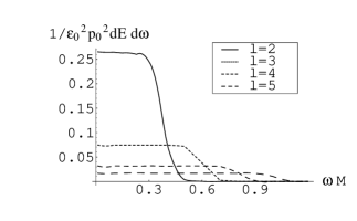
Figure 2: The energy spectra for the four lowest radiatable multipoles, for a massless particle falling from infinity into a Schwarzschild black hole.

Let us now make the bridge between these results and previous results on collisions between massive particles at nearly the speed of light ruffini ; D'Eath ; smarr2 . As we mentioned, putting $p_{0}\rightarrow m_{0}$ and $\epsilon_{0}\rightarrow\gamma$ does the trick. So for ultrarelativistic test particles with mass $m_{0}$ falling into a Schwarzschild black hole, one should have $(dE/d\omega)_{\omega=0}=0.4244m_{0}^{2}\gamma^{2}$ and $\Delta E=0.262\frac{m_{0}^{2}\gamma^{2}}{M}$. Smarr smarr2 obtains

$$\left(\frac{dE}{d\omega}\right)^{\rm Smarr}_{\omega=0}=\frac{8}{6\pi}m_{0}^{2}\gamma^{2}\sim 0.4244m_{0}^{2}\gamma^{2}\,,$$

$$\Delta E_{\rm Smarr}=0.2\frac{m_{0}^{2}\gamma^{2}}{M}\,.$$ (19)

So Smarr’s result for the ZFL is in excellent agreement with ours, while his result for the total energy radiated is seen to be an underestimate. As we know from the work of Davis et al davis for a particle falling from infinity with $v_{\infty}=0$ most of the radiation is carried by the $l=2$ mode. Not so here, in fact in our case less than 50% is carried in the quadrupole mode (we obtain $\Delta E_{l=2}=0.1\frac{\epsilon_{0}^{2}p_{0}^{2}}{M}$, $\Delta E_{l=3}=0.0447\frac{\epsilon_{0}^{2}p_{0}^{2}}{M}$ ). This is reflected in the angular distribution of the radiated energy (power per solid angle)

$$\frac{dE}{d\Omega}=\Delta E_{l}\frac{(l-2)!}{(l+2)!}\left[2\frac{\partial^{2}}{\partial\theta^{2}}Y_{l0}+l(l+1)Y_{l0}\right]^{2},$$ (20)

which we plot in Figure 3. Compare with figure 5 of smarr2 .

Figure 3: The energy radiated per solid angle as a function of $\theta$.

If, as Smarr, we continue to assume that something deep is at work, and that these results can be carried over to the case of two equal mass black holes flying towards each other at (close to) the speed of light, we obtain a wave generation efficiency of 13 %. This is in close agreement with results by D’Eath and Payne D'Eath ; payne , who obtain a 16% efficiency (Smarr’s results cannot be trusted in this regime, as shown by Payne payne2 ). Now, D’Eath and Payne’s results were achieved by cutting an infinite series for the news function at the second term, so one has to take those results with some care. However, the agreement we find between ours and their results lead us to believe that once again perturbation theory has a much more wider realm of validity. To our knowledge, this is the first alternative to D’Eath and Payne’s method of computing the energy release in such events.

This work was partially funded by Fundação para a Ciência e Tecnologia (FCT) through project PESO/PRO/2000/4014. V.C. also acknowledges finantial support from FCT through PRAXIS XXI programme. J. P. S. L. thanks Observatório Nacional do Rio de Janeiro for hospitality.

References

- (1) K. Danzmann et al., in Gravitational Wave Experiments, eds. E. Coccia, G. Pizzella and F. Ronga (World Scientific, Singapore, 1995).
- (2) A. Abramovici et al., Science 256, 325 (1992).
- (3) C. Bradaschia et al., in Gravitation 1990, Proceedings of the Banff Summer Institute, Banff, Alberta, 1990, edited by R. Mann and P. Wesson (World Scientific, Singapore, 1991)
- (4) P. Anninos, D. Hobill, E. Seidel, L. Smarr, and W. M. Suen, Phys. Rev. Lett. 71, 2851 (1993); P. Anninos and S. Brandt, Phys. Rev. Lett. 81, 508 (1998).
- (5) R. J. Gleiser, C. O. Nicasio, R. H. Price, and J. Pullin, Phys. Rev. Lett. 77, 4483 (1996).
- (6) S. L. Smarr (ed.), Sources of Gravitational Radiation, (Cambridge University Press, 1979).
- (7) F. Zerilli, Phys. Rev. D 2, 2141 (1970).
- (8) M. Davis, R. Ruffini, W. H. Press, and R. H. Price, Phys. Rev. Lett. 27, 1466 (1971).
- (9) R. Ruffini, Phys. Rev. D 7, 972 (1973).
- (10) C. O. Lousto, and R. H. Price, Phys. Rev. D 55, 2124 (1997); K. Martel, and E. Poisson, gr-qc/0107104.
- (11) P. D. D’Eath, in Black Holes: gravitational interactions, (Clarendon Press, Oxford, 1996).
- (12) L. Smarr, Phys. Rev. D 15, 2069 (1977).
- (13) S. Dimopoulos, and G. Landsberg, Phys. Rev. Lett. 87,161602 (2001); S. B. Giddings, and S. Thomas, hep-ph/0106219, v2.
- (14) D. M. Eardley and S. B. Giddings, gr-qc/0201034.
- (15) S. N. Solodukhin, hep-ph/0201248.
- (16) P. D. D’Eath and P. N. Payne, Phys. Rev. D 46, 658 (1992); Phys. Rev. D 46, 675 (1992); Phys. Rev. D 46, 694 (1992);
- (17) T. Regge and J. A. Wheeler, Phys. Rev. 108, 1063 (1957).
- (18) F. Zerilli, Phys. Rev. Lett. 24, 737 (1970).
- (19) V. Ferrari and R. Ruffini, Phys. Lett. B 98, 381 (1981).
- (20) S. Chandrasekhar, and S. Detweiler, Proc. R. Soc. London A 344, 441 (1975);
- (21) V. Ferrari and B. Mashhoon, Phys. Rev. Lett. 52, 1361 (1984).
- (22) B. F. Schutz and C. M. Will, Ap. J. 291, L33 (1985).
- (23) P. N. Payne, Phys. Rev. D 28, 1894 (1983);