The Structure of the Big Bang from
Higher-Dimensional Embeddings

Abstract

We give relations for the embedding of spatially-flat Friedmann-Robertson-Walker cosmological models of Einstein’s theory in flat manifolds of the type used in Kaluza-Klein theory. We present embedding diagrams that depict different 4D universes as hypersurfaces in a higher dimensional flat manifold. The morphology of the hypersurfaces is found to depend on the equation of state of the matter. The hypersurfaces possess a line-like curvature singularity infinitesimally close to the $t=0^{+}$ 3-surface, where $t$ is the time expired since the big bang. The family of timelike comoving geodesics on any given hypersurface is found to have a caustic on the singular line, which we conclude is the 5D position of the point-like big bang.

I Introduction

In four-dimensional general relativity as formulated by Einstein, the singularity theorems tell us that the big bang was a unique birth event for a universe whose matter is of the conventional sort and obeys the energy conditions Haw73 ; Wal84 . The early stages of the standard Friedmann-Robertson-Walker (FRW) models may be modified by inflation, basically because then there is a period when the energy conditions are violated Lin90 ; Wes99 . The associated process of mass generation can either be described at the particle level by quantum field theory or at the macroscopic level by classical theory Lin79 ; Bro79 ; Gut81 ; Hen83 ; Bon60 ; Wes85 . The early stages of standard cosmology may also be modified by the effects of quantum gravity and quantum tunneling Gib93 ; Vil82 . In this regard, the appropriate formalism in 4D for early times can be investigated by considering the problem in 5D Dar00 . Also, the status of standard cosmological models for late times can be clarified by considering how they are embedded in 5D Lid97 . There has recently been renewed interest in 5D manifolds of the type used originally in Kaluza-Klein theory Wes99 ; App87 . This is partly because of the resurrection of Campbell’s theorem, which ensures a perfect local embedding of a 4D Einstein space in a 5D Kaluza-Klein space Cam26 ; Rip95 ; Rom96 ; and partly because of the implications of higher-dimensional approaches such as superstrings and supergravity Wit81 ; West86 ; Gre87 ; Duf96 as well as string and membrane theory You00 ; Maa00 ; Cha00 . Recently, several authors have revisited the problem of embedding 4D FRW metrics in 5D Minkowski space with an eye towards determining the geometrical structure of the big bang Lyn89 ; Rin00 . For the standard spatially-flat ($k=0$) 4D FRW models the appropriate class of 5D models was given in a notable paper by Ponce de Leon Pon88a . His models are separable in time $t$, space $\sigma$, and an extra coordinate $\ell$, and reduce to the FRW ones on $\ell$ = constant hypersurfaces (henceforth denoted by $\Sigma_{\ell}$). Interesting work has been done on those and related models, both from the astrophysical side Wes92 ; Wes94 ; Wes95 and the mathematical side McM94 ; Col95 ; Abo96 . One of the Ponce de Leon 5D solutions when unembedded is the 4D Einstein-de Sitter solution, which is in tolerable agreement with observations; but surprisingly this and other Ponce de Leon solutions have been shown by fast algebraic computer package Lak95 to be flat in 5D. This may appear unusual, but recent work has made it clear that a flat and apparently empty 5D manifold may contain a curved, 4D manifold Wes99 ; Lid97 ; McM94 ; Col95 ; Abo96 ; Liu95 ; Wes00 . However, while much work has been done on the 5D Ponce de Leon solutions, no systematic account has been given of how they embed the 4D big bang.

The present paper addresses this issue. The plan of the paper is as follows: Section II introduces the Ponce de Leon class of one-parameter 5D cosmological solutions to the vacuum Einstein field equations. $\Sigma_{\ell}$ hypersurfaces are shown to be geometrically identical to spatially flat ($k=0$) FRW cosmological models. The type of matter in these complementary 4D models is determined by the value of the parameter $\alpha$, and includes both inflationary and non-inflationary cases. The 5D manifold is then shown to be identical to Minkowski space ${\mathbb{M}}_{5}$ via a coordinate transformation. This coordinate transformation allows us to plot our universe as a hypersurface in a 3D Cartesian space once angular variables are suppressed, which is the subject of section III. Subsection III.1 deals with analytically determining where comoving observers on $\Sigma_{\ell}$ emanate from in ${\mathbb{M}}_{5}$ as $t\rightarrow 0^{+}$, which corresponds to a singularity in the 4-geometry. Subsection III.2 demonstrates that the local geometry of $\Sigma_{\ell}$ around regular points is elliptical for non-inflationary cases and hyperbolic for inflationary ones. Subsection III.3 establishes some results concerning the global properties of the $\Sigma_{\ell}$ foliation of ${\mathbb{M}}_{5}$, the main conclusion being that the cosmological coordinates used in the Ponce de Leon metric do not cover all of 5D Minkowski space. Subsection III.4 presents computer plots of $\Sigma_{\ell}$ hypersurfaces for a wide variety of cases. These plots are discussed in subsection III.5. Also in this subsection, a detailed analysis of the singular points on $\Sigma_{\ell}$ is presented. We find that there is a line-like curvature singularity on $\Sigma_{\ell}$, but that the big bang corresponds to only one point on that line. Section IV discusses special cases of the Ponce de Leon class not mentioned in other sections and the corresponding 4D universes. Section V contains our concluding remarks.

Conventions.

Throughout the paper, the 5D metric signature is taken to be $(+----)$, while the choice of 4D metric signature is $(+---)$. The spacetime coordinates are labeled $x^{0}=t$, $x^{i}=(r,\theta,\phi)$. The extra coordinate is $x^{4}=\ell$. The range of tensor indices is as follows: $A,B,\ldots=0-4$; $\alpha,\beta,\ldots=0-3$; and $a,b=0,1$. $\nabla_{A}$ indicates the 5D covariant derivative. We denote the metric of flat 3-space by $d\sigma^{2}=dr^{2}+r^{2}\,d\Omega^{2}$ with $d\Omega^{2}=d\theta^{2}+\sin^{2}\theta\,d\phi^{2}$. Finally, we use geometric units where $c=G=1$.

II Ponce de Leon Cosmologies

The standard class of Ponce de Leon cosmological solutions is flat in ordinary 3D space, curved in 4D spacetime and flat in 5D Pon88a ; Wes92 ; Wes94 ; Wes95 ; McM94 ; Col95 ; Abo96 . It has a 5D line element

$$dS^{2}=\ell^{2}\,dt^{2}-t^{2/\alpha}\ell^{2/(1-\alpha)}\,d\sigma^{2}-\alpha^{2}(1-\alpha)^{-2}t^{2}\,d\ell^{2}.$$ (1)

This metric is an exact solution of the 5D field equations in apparent vacuum, which in terms of the Ricci tensor are $R_{AB}=0$. In what follows, we will examine the $\Sigma_{\ell}$ hypersurfaces of (1) in detail. The induced metric $h_{\alpha\beta}$ on these hypersurfaces is given by

$$ds^{2}=h_{\alpha\beta}dx^{\alpha}dx^{\beta}=\ell^{2}dt^{2}-t^{2/\alpha}\ell^{2/(1-\alpha)}d\sigma^{2},$$ (2)

which we can, of course, identify with the line element of a spatially-flat ($k=0$) FRW cosmology with scale factor

$$a(\tau)=\ell^{(2\alpha-1)/\alpha(1-\alpha)}\tau^{1/\alpha},$$ (3)

where $\tau=\ell t$ corresponds to the FRW clock time. That is, the geometry of each of the $\Sigma_{\ell}$ 4-surfaces is identical to geometry of the 4D spacetime models commonly used to describe our universe.

We can use the form of the induced metric (2) to calculate the 4D Einstein tensor $G_{\alpha\beta}$ on each of the $\Sigma_{\ell}$ surfaces. Alternatively, we can use standard techniques to break the 5D field equations $R_{AB}=0$ into one wave equation, four conservation equations and ten equations for the components of $G_{\alpha\beta}$ Wes99 ; Lid97 ; Cam26 . The latter are given in general by

$$G_{\alpha\beta} = \frac{\Phi_{;\alpha\beta}}{\Phi}+\frac{1}{2\Phi^{2}}\bigg{\{}\frac{\Phi^{*}g^{*}_{\alpha\beta}}{\Phi}-\frac{g^{\mu\nu}g^{*}_{\mu\nu}g^{*}_{\alpha\beta}}{2}+g^{\lambda\mu}g^{*}_{\alpha\lambda}g^{*}_{\beta\mu}$$ (4)

$$-g^{**}_{\alpha\beta}+\frac{g_{\alpha\beta}}{4}\left[g^{*\mu\nu}g^{*}_{\mu\nu}+\left(g^{\mu\nu}g^{*}_{\mu\nu}\right)^{2}\right]\bigg{\}},$$

where $g_{44}=-\Phi^{2}$, and a star (^∗) denotes $\partial/\partial\ell$. We now ask the question: what kind of 4D matter would give rise to such an Einstein tensor? To answer, we must associate $G_{\alpha\beta}$ with a stress-energy tensor $T_{\alpha\beta}$ via the Einstein equations $G_{\alpha\beta}=8\pi T_{\alpha\beta}$. For the Ponce de Leon solutions, this “induced” stress-energy tensor is of the perfect-fluid type with the density and pressure of the “induced” matter given by:

$$8\pi\rho=\frac{3}{\alpha^{2}\tau^{2}},\quad 8\pi p=\frac{2\alpha-3}{\alpha^{2}\tau^{2}}.$$ (5)

It should be stressed that this density and pressure refers to a 4D matter distribution that gives rise to a curved 4D manifold, via the Einstein equation, geometrically identical to the $\Sigma_{\ell}$ hypersurfaces. We have not inserted any matter into the 5D manifold by hand, as is commonly done in the brane-world/thin-shell formalism where the 5D stress-energy is a discontinuous, distribution-valued tensor field. It is for this reason that we call the matter described by $T_{\alpha\beta}$ induced; rather than being inserted into the Einstein equations as an external source for the gravitational field, the matter distribution is fixed by the morphology of the $\Sigma_{\ell}$ surfaces and the higher-dimensional geometry.

The equation of state of the induced matter is

$$p=(2\alpha/3-1)\rho,$$ (6)

which is determined by the dimensionless parameter $\alpha$ in the metric (1). For $\alpha=3/2$, $8\pi\rho=4/3\tau^{2}$ and $p=0$, which describes the late (dust) universe. For $\alpha=2$, $8\pi\rho=3/4\tau^{2}$ and $8\pi p=1/4\tau^{2}$ so $p=\rho/3$, which describes the early (radiation) universe. That these quantities are the same as they are in the 4D FRW models should not surprise us, as this could be inferred from Campbell’s theorem Wes99 ; Lid97 ; Cam26 . However, the Ponce de Leon class of solutions also embeds some more exotic cosmological scenarios. To see this, let us form the gravitational density of the induced matter,

$$\rho_{g}=\rho+3p=\frac{3(\alpha-1)}{4\pi\alpha^{2}\tau^{2}}.$$ (7)

The strong energy condition demands that $\rho_{g}\geq 0$, which is only satisfied for $\alpha\geq 1$. For cases which violate this condition $\alpha\in(0,1)$, the Raychaudhuri equation says that geodesics paths on $\Sigma_{\ell}$ accelerate away from one another, as is expected in inflationary scenarios. This is easily verified by examining the congruence of comoving $d\sigma=0$ paths in the 4-geometry described by (2). Just like in conventional FRW cosmology, the proper distance between adjacent paths will increase at an accelerating pace if the deceleration parameter,

$$q(\tau)\equiv-a\frac{d^{2}a}{d\tau^{2}}\left(\frac{da}{d\tau}\right)^{-2}=\alpha-1,$$ (8)

is negative. We therefore conclude that models with $\alpha\in(0,1)$ describe inflationary situations where the cosmological fluid has repulsive properties, while models with $\alpha>1$ have ordinary gravitating matter. Note that we exclude models with $\alpha<0$ because they imply a contracting universe.

As a quick aside, we note that the Ponce de Leon metrics (1) have a constrained equation of state (i.e., the type of matter corresponding to the curvature of the $\Sigma_{\ell}$ hypersurfaces does not change in time). If one wanted to study a more realistic model of our universe, the radiation-matter transition could be generated by joining metrics with $\alpha=2$ and $\alpha=3/2$ across a $t=$ constant hypersurface that represents the surface of last scattering. Such a calculation is, however, beyond the scope of this paper.

It was discovered by computer that (1) is actually flat in 5D Wes92 ; Wes94 ; Wes95 ; McM94 ; Col95 ; Abo96 ; Lak95 . To prove this algebraically is non-trivial, but we can change coordinates from those in (1) to

$$T(t,r,\ell) = \frac{\alpha}{2}\left(1+\frac{r^{2}}{\alpha^{2}}\right)t^{1/\alpha}\ell^{1/(1-\alpha)}$$ (9a)

$$- \frac{\alpha}{2}\frac{\left[t^{-1}\ell^{\alpha/(1-\alpha)}\right]^{(1-2\alpha)/\alpha}}{1-2\alpha},$$

$$R(t,r,\ell) = rt^{1/\alpha}\ell^{1/(1-\alpha)},$$ (9b)

$$L(t,r,\ell) = \frac{\alpha}{2}\left(1-\frac{r^{2}}{\alpha^{2}}\right)t^{1/\alpha}\ell^{1/(1-\alpha)}$$ (9c)

$$+ \frac{\alpha}{2}\frac{\left[t^{-1}\ell^{\alpha/(1-\alpha)}\right]^{(1-2\alpha)/\alpha}}{1-2\alpha}.$$

Then (1) becomes

$$dS^{2}=dT^{2}-\left(dR^{2}+R^{2}\,d\Omega^{2}\right)-dL^{2},$$ (10)

which is 5D Minkowski ${\mathbb{M}}_{5}$. In order to contrast with the standard coordinates $x^{A}=(t,r,\theta,\phi,\ell)$, we will label the Minkowski coordinates as $y^{A}=(T,R,\theta,\phi,L)$. The importance of (9) is that it allows us to visualize the geometric structure of our universe when viewed from 5D flat space by plotting the surfaces defined by $\ell=$ constant. As seen in equation (2) above, these hypersurfaces share the same intrinsic geometry as standard 4D FRW $k=0$ cosmologies, which means that they are equivalent to such models in a mathematical sense (this is the paradigm commonly adopted when one tries to embed known solutions of the Einstein equation in higher-dimensional manifolds Lyn89 ; Rin00 ). We can therefore learn a great deal about the local and global topological properties of 4D FRW models, as well as the geometric structure of the “physical” big bang, from studying the $\Sigma_{\ell}$ hypersurfaces. These and other issues are considered in the following sections.

III The Structure of the Embedded Universes

In order to analyze the geometrical properties of the $\Sigma_{\ell}$ hypersurfaces, we note that the $T$, $R$, $L$ coordinates of (10) are orthogonal and so can be used as Cartesian axes. Then, the universe will have a shape defined by $T=T(t,r,\ell_{0})$, $R=R(t,r,\ell_{0})$, $L=L(t,r,\ell_{0})$ on some hypersurface $\ell=\ell_{0}$. The following three subsections III.1 – III.3 explore various characteristics of the $\Sigma_{\ell}$ hypersurfaces analytically. The goal is to get a feel for the geometry of the $\Sigma_{\ell}$ hypersurfaces before computer plots are presented in subsection III.4. In that subsection, we plot hypersurfaces for several different cases, suppressing the $\theta$ and $\phi$ coordinates so that our universe appears as a 2-surface embedded in Euclidean 3-space ${\mathbb{E}}_{3}$. Subsection III.5 deals with the location and five-dimensional shape of the big-bang singularity, and is in some sense a continuation of the discussion of singular points started in subsection III.1.

III.1 Properties of Singular Points on $\Sigma_{\ell}$

In this subsection, we will begin to investigate singularities on the $\Sigma_{\ell}$ hypersurfaces, and introduce the problem of locating where these singularities occur in ${\mathbb{M}}_{5}$. Our goal is to get a feel for the shape of the $\Sigma_{\ell}$ surfaces using analytical methods before resorting to the computer plotting of subsection III.4.

A cursory inspection of equation (2) reveals what appears to be a singularity in the 4-geometry at $t=0$, which is commonly associated with the big bang. We can calculate the 4D Kretschmann scalar (or curvature invariant) of the $\ell=\ell_{0}$ hypersurfaces:

$$K=R^{\alpha\beta\gamma\delta}R_{\alpha\beta\gamma\delta}=\frac{12\left(\alpha^{2}-2\alpha+2\right)}{\ell_{0}^{4}\alpha^{4}t^{4}}.$$ (11)

We note that $K$ diverges for all $\alpha$ at $t=0$. This implies that the anomaly at $t=0$ is a genuine curvature singularity in the 4D manifold represented by (2). However, we know that the 5D manifold (1) has $R_{ABCD}=0$ and is therefore devoid of any singularities. Therefore, the 4D big bang results from the nature of the $\Sigma_{\ell}$ hypersurfaces, or equivalently the choice of 5D coordinates.

The question naturally arises of where the big bang at $t=0$ appears in ${\mathbb{M}}_{5}$. One way to approach the problem is to take the $t\rightarrow 0^{+}$ limit of the coordinate transformation (9) while holding $r$ constant. It transpires that there are two different physically interesting cases:

$$\lim_{t\rightarrow 0^{+}}T(t,r,\ell) = -\frac{\alpha}{2(1-2\alpha)}\left[\frac{\ell^{\alpha/(1-\alpha)}}{t}\right]^{(1-2\alpha)/\alpha}$$ (12a)

$$\rightarrow \begin{cases}0,&\alpha\in(\tfrac{1}{2},\infty)\\ -\infty,&\alpha\in(0,\tfrac{1}{2})\end{cases}$$

$$\lim_{t\rightarrow 0^{+}}R(t,r,\ell) = 0,\quad\alpha>0$$ (12b)

$$\lim_{t\rightarrow 0^{+}}L(t,r,\ell) = +\frac{\alpha}{2(1-2\alpha)}\left[\frac{\ell^{\alpha/(1-\alpha)}}{t}\right]^{(1-2\alpha)/\alpha}$$ (12c)

$$\rightarrow \begin{cases}0,&\alpha\in(\tfrac{1}{2},\infty)\\ +\infty,&\alpha\in(0,\tfrac{1}{2})\end{cases}.$$

In other words, the congruence of $(r,\theta,\phi)=$ constant curves on $\Sigma_{\ell}$ (henceforth denoted by $\gamma_{r}$) converges to a point as $t\rightarrow 0^{+}$ for all $\alpha>0$. For $\alpha\in(\tfrac{1}{2},\infty)$ the caustic is at $T=R=L=0$; for $\alpha\in(0,\tfrac{1}{2})$, the caustic is at null infinity as approached by following the ray $T+L=R=0$ into the past. Naïvely, this would seem to suggest that the the big bang is a point-like event in 5D. However, caution is warranted because the limiting procedure described above is not unique. In particular, we need not approach $t=0$ in a manner that leaves $r=$ constant. For example, suppose we follow the path $r(t)\propto t^{-1/2\alpha}$ into the past. If $\alpha\in(\tfrac{1}{2},\infty)$, then we will end up at the 5D point $T=-L=\text{constant}\neq 0$, $R=0$, which is different from the caustic in the $\gamma_{r}$ congruence. So, it is not correct to uniquely associate $t=0$ with the position of the $\gamma_{r}$ caustic. In general, there are many points on $\Sigma_{\ell}$ eligible for that distinction. On the other hand, it should be stressed that if we approach the initial singularity along any path where $r(t)$ tends to a finite constant as $t\rightarrow 0^{+}$, then we will end up at one of the $\gamma_{r}$ caustics (which one, depends on the value of $\alpha$). The issue of the precise location of the big bang in 5D is complicated, so we will defer a full discussion until subsection III.5.

Regardless of where the $t=0$ surface lies in ${\mathbb{M}}_{5}$, the calculations presented in this section demonstrate that the point $T=R=L=0$ is a special point for $\alpha\in(\tfrac{1}{2},\infty)$, and that a point at null infinity $T=-L\rightarrow-\infty,R=0$ is a special point for $\alpha\in(0,\tfrac{1}{2})$. The computer-generated figures presented in subsection III.4 will bear out this analytical conclusion.

III.2 Properties of Regular Points on $\Sigma_{\ell}$

Having already given a partial discussion of the singular points on the $\Sigma_{\ell}$ hypersurfaces, we would now like to concentrate on analytically determining what $\Sigma_{\ell}$ looks like in the neighborhood of regular points. As mentioned above, our plots of $\Sigma_{\ell}$ will look like 2-surfaces embedded in ${\mathbb{E}}_{3}$. It is therefore useful to recall the notion of the Gaussian curvature $G^{\mathbb{E}}$ of 2-surfaces $S\in{\mathbb{E}}_{3}$ from standard differential geometry Lip69 . Consider a point $P$ on a surface $S$ embedded in ${\mathbb{E}}_{3}$. In a small neighborhood around $P$, the surface $S$ can be modeled as a paraboloid centered at $P$ (the so-called “osculating paraboloid”). The shape of this paraboloid is given by the sign of the Gaussian curvature, which in turn is given by the product of the principle curvatures of $S$ at $P$. If $G^{\mathbb{E}}>0$, the paraboloid is elliptical and the surface has a convex or concave shape about $P$. If $G^{\mathbb{E}}<0$, the paraboloid is hyperbolic and the local shape of $S$ is that of the familiar “saddle-surface”. If $G^{\mathbb{E}}=0$, one or both of the principle curvatures are zero implying a cylindrical or planar shape. In terms of intrinsic geometrical quantities, the Gaussian curvature is given by

$$G^{\mathbb{E}}=\frac{{}^{(2)}R^{\mathbb{E}}_{0101}}{\det[{}^{(2)}g^{\mathbb{E}}_{ab}]},$$ (13)

where ${}^{(2)}g^{\mathbb{E}}_{ab}$ is the Euclidean 2-metric on $S$ and ${}^{(2)}R^{\mathbb{E}}_{1212}$ is the single independent component of the associated 2D Riemann-Christoffel tensor. For the Euclidean version of the $\Sigma_{\ell}$ hypersurfaces, we can find ${}^{(2)}g^{\mathbb{E}}_{ab}$ from the positive-definite line element

$${}^{(2)}g^{\mathbb{E}}_{ab}dx^{a}dx^{b}=\left(dT^{2}+dR^{2}+dL^{2}\right)\Big{|}_{d\ell=0}.$$ (14)

Using this, we can calculate the Gaussian curvature (13) of the $\Sigma_{\ell}$ surfaces when embedded in Euclidean space:

$$G^{\mathbb{E}}=\frac{4\alpha^{6}(\alpha-1)t^{2(\alpha-2)/\alpha}\ell^{-2(1+\alpha)/(1-\alpha)}}{\left[\chi^{2}-2r^{2}\chi+(r^{2}+\alpha^{2})^{2}\right]^{2}},$$ (15a)

where

$$\chi\equiv\alpha^{2}t^{2(\alpha-1)/\alpha}\ell^{2\alpha/(\alpha-1)}.$$ (15b)

We note that the denominator of $G^{\mathbb{E}}$ is positive definite for all values of $t$, $r$, $\ell$ and $\alpha$. Therefore, $G^{\mathbb{E}}>0$ for $\alpha\in(1,\infty)$ and $G^{\mathbb{E}}<0$ for $\alpha\in(0,1)$ for all $(t,\ell)>0$. In other words, when viewed in ${\mathbb{E}}_{3}$, all the non-singular points on $\Sigma_{\ell}$ are elliptical for non-inflationary models and hyperbolic for inflationary ones.

We mention in passing that it is also possible to calculate the Gaussian curvature $G^{\mathbb{M}}$ of the $\Sigma_{\ell}$ surfaces when they are embedded in ${\mathbb{M}}_{3}$. The 2-metric ${}^{(2)}g_{ab}^{\mathbb{M}}$ is obtained by setting $d\theta=d\phi=d\ell=0$ in (1). This yields

$$G^{\mathbb{M}}=\frac{{}^{(2)}R^{\mathbb{M}}_{0101}}{\det[{}^{(2)}g^{\mathbb{M}}_{ab}]}=\frac{\alpha-1}{\alpha^{2}t^{2}\ell^{2}},$$ (16)

which, like $G^{\mathbb{E}}$, is positive for $\alpha\in(1,\infty)$ and negative for $\alpha\in(0,1)$. Also, we note that $G^{\mathbb{M}}$ diverges as $t\rightarrow 0^{+}$ for all $\alpha$, which is consistent with the behaviour of the 4D Kretschmann scalar (11) calculated above. The Ricci tensor in 2D is given by ${}^{(2)}R_{ab}^{\mathbb{M}}={}^{(2)}g_{ab}^{\mathbb{M}}G^{\mathbb{M}}$, so that the strong energy condition reads ${}^{(2)}R_{ab}^{\mathbb{M}}u^{a}u^{b}=G^{\mathbb{M}}\geq 0$ where $u^{a}$ is some timelike 2-velocity. Hence, if $G^{\mathbb{M}}<0$ then the strong energy condition is violated in 2D. This implies that the 2D gravitational density of the matter is less than zero, which in turn means that the relative velocity between neighboring timelike geodesics is increasing in magnitude by Raychaudhuri’s equation. This is consistent with the finding that $q(t)<0$ and $\rho+3p<0$ for $\alpha\in(0,1)$ discussed in subsection II.

In conclusion, we have found out that the local geometry around regular points on $\Sigma_{\ell}$ – for a given value of $\alpha$ – is determined by whether or not the model represents a universe with ordinary or inflationary matter. In the former case the regular points are elliptical, in the latter case they are hyperbolic.

III.3 Global Properties of $\Sigma_{\ell}$

In the previous two subsections, we have discussed the properties of singular and regular points on $\Sigma_{\ell}$. We now turn our attention to the global properties of the hypersurfaces, with an eye to determining which portion of ${\mathbb{M}}_{5}$ they inhabit. In other words, we want to know what part of the ${\mathbb{M}}_{5}$ manifold is covered by the $x^{A}=(t,r,\theta,\phi,\ell)$ coordinates.

The coordinate transformation (9) implies

$$(T+L)/R=\alpha/r.$$ (17)

Since $R/r$ is positive for $(t,\ell)>0$ and we assume that $\alpha>0$, this implies that the $\Sigma_{\ell}$ hypersurfaces are restricted to the half of the manifold defined by $(T+L)>0$. Next, the transformation also implies that

$$T^{2}-R^{2}-L^{2}=\frac{\alpha^{2}t^{2}\ell^{2}}{2\alpha-1}.$$ (18)

Hence, if $\alpha\in(\tfrac{1}{2},\infty)$ then the $\Sigma_{\ell}$ surfaces must lie in the region satisfying $T^{2}-R^{2}-L^{2}>0$, which is the volume inside the light cone originating from $T=R=L=0$. If $\alpha\in(0,\tfrac{1}{2})$, the surfaces must lie in the region outside the light cone, defined by $T^{2}-R^{2}-L^{2}<0$. Also, the $\Sigma_{\ell}$ surfaces approach $T^{2}-R^{2}-L^{2}=0$ as $\ell\rightarrow 0$, implying that the direction of increasing $\ell$ is always away from the light cone. Putting these facts together, we see that if $\alpha\in(\tfrac{1}{2},\infty)$, then the coordinates utilized in (1) only cover the portion of ${\mathbb{M}}_{5}$ inside the light cone centered at the origin with $T>0$. If $\alpha\in(0,\tfrac{1}{2})$, then the coordinates in (1) cover the region of ${\mathbb{M}}_{5}$ satisfying $(T+L)>0$ and exterior to the light cone centered at the origin. Finally, equations (9b), (17) and (18) can be rearranged to yield

$$0=UV-\frac{\alpha^{2(1-\alpha)}\ell^{2(1-2\alpha)/(1-\alpha)}U^{2\alpha}}{(2\alpha-1)}-R^{2},$$ (19)

where we have introduced the advanced and retarded coordinates

$$U=T+L,\quad V=T-L.$$ (20)

This defines the $\Sigma_{\ell}$ hypersurfaces entirely in terms of the $y^{A}$ coordinates and $\ell$. This is a useful relationship which we will need below.

To conclude, we have discovered that the $\Sigma_{\ell}$ hypersurfaces are constrained to lie in one half of ${\mathbb{M}}_{5}$ for all $\alpha>0$. Furthermore, they must lie within the light cone centered at the origin for $\alpha\in(\tfrac{1}{2},\infty)$ and outside it for $\alpha\in(0,\tfrac{1}{2})$. We have summarized all that we have learned about the effects of $\alpha$ on the $\Sigma_{\ell}$ hypersurfaces in Table 1.

$\alpha$ interval	sign of $q(\tau)$	osculating paraboloid	caustic location	$T^{2}-R^{2}-L^{2}$
$(0,\tfrac{1}{2})$	$-$	hyperbolic	null infinity	$-$
$(\tfrac{1}{2},1)$	$-$	hyperbolic	origin	$+$
$(1,\infty)$	$+$	elliptical	origin	$+$

Table 1: Dynamical and topological properties of cosmologies embedded on $\Sigma_{\ell}$ hypersurfaces. The “caustic location” refers to the point that the $\gamma_{r}$ lines approach as $t\rightarrow 0^{+}$.

III.4 Visualization of the $\Sigma_{\ell}$ hypersurfaces

We are now in a position to discuss Figures 1 – 5 in detail. The plots show the constant $t$ and $r$ coordinate lines associated with a given $\Sigma_{\ell}$ hypersurface (denoted by $\gamma_{t}$ and $\gamma_{r}$ respectively) as viewed from the $(T,R,L)$ space. As an aid to visualization, we choose to let $r$ and $R$ range over both positive and negative numbers, so the $\Sigma_{\ell}$ hypersurfaces are symmetric about the $R=0$ plane (if it is desired to have $r>0$ or $R>0$ one of the symmetric halves can be deleted). As the models evolve in $t$-time they will generally grow in the $R$-direction, so that the $\Sigma_{\ell}$ hypersurfaces appear to “open-up” in the direction of increasing $T$. The $\gamma_{t}$ isochrones are seen to wrap around the hypersurfaces such that they cross the $R=0$ plane perpendicularly. The $\gamma_{r}$ lines are orthogonal (in a Euclidean sense) to $\gamma_{t}$ lines at $R=0$ and run along the length of the surface.

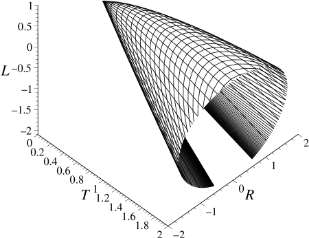
Figure 1: $\Sigma_{\ell}$ hypersurface with $\alpha=3/2$ and $\ell_{0}=1$. We take $t\in[10^{-400},2]$ and $r\in[-10,10]$, with $\Delta t\approx 0.01$ and $\Delta r\approx 0.003$.

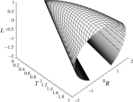
Figure 2: $\Sigma_{\ell}$ hypersurface with $\alpha=2$ and $\ell_{0}=1$. We take $t\in[10^{-400},2]$ and $r\in[-10,10]$, with $\Delta t\approx 0.01$ and $\Delta r\approx 0.003$.

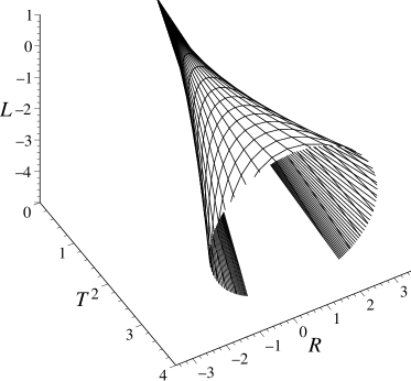
Figure 3: $\Sigma_{\ell}$ hypersurface with $\alpha=2/3$ and $\ell_{0}=1$. We take $t\in[10^{-600},8]$ and $r\in[-3,3]$, with $\Delta t\approx 0.3$ and $\Delta r\approx 0.08$.

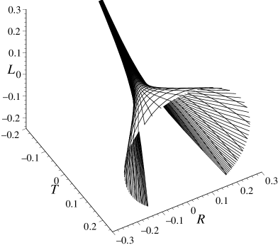
Figure 4: $\Sigma_{\ell}$ hypersurface with $\alpha=1/30$ and $\ell_{0}=1$. We take $t\in[0.9,1.1]$ and $r\in[-0.1,0.1]$, with $\Delta t\approx 0.01$ and $\Delta r\approx 0.003$.

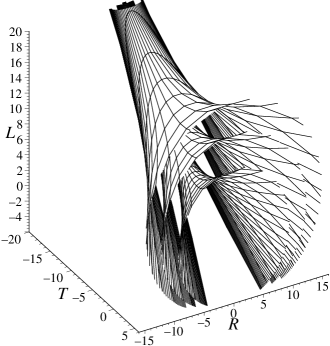
Figure 5: $\Sigma_{\ell}$ hypersurfaces with $\alpha=1/3$ and $\ell_{0}=20,40,60$. We take $t\in[10^{-300},3]$ and $r\in[-2,2]$, with $\Delta t\approx 0.05$ and $\Delta r\approx 0.07$.

When using a computer to plot the surfaces, it is necessary to choose finite ranges of $t$ and $r$. The ranges used in each of the Figures are given in the captions, along with the increments in the time or radial coordinates between adjacent coordinate lines (denoted by $\Delta t$ and $\Delta r$ respectively). For models with $\alpha\in(\tfrac{1}{2},\infty)$, the $t=0$ “line” is really a point for finite values of $r$. Therefore, the first $\gamma_{t}$ line in such plots has been chosen to be $t=\delta$, where $\delta$ is the smallest positive number allowed by machine precision. For such models, the lower edge of the $\Sigma_{\ell}$ hypersurfaces corresponds to the $t=\delta$ line. For plots with $\alpha\in(0,\tfrac{1}{2})$ we have chosen to restrict $t$ and $r$ to a fairly narrow ranges in order to facilitate visualization. As a result of this, the lower edges of $\Sigma_{\ell}$ in such plots are the $\gamma_{r}$ curves with the largest value of $|r|$. However, we have confirmed that if the range of $r$ is larger and $\min(t)=\delta$, then the comoving trajectories with the largest values of $|r|$ tend to bunch up along the $t=\delta$ line. That is, if the range of $r$ is unrestricted then the lower edge of the $\Sigma_{\ell}$ hypersurfaces will correspond to the $\gamma_{t}$ line closest to the big bang, irrespective of the value of $\alpha$.

We have carried out an extensive analysis of the morphology of the $\Sigma_{\ell}$ hypersurfaces in the $(\alpha,\ell_{0})$ parameter space, and present five informative cases which are illustrated in the Figures:

Model 1:

$\alpha=3/2$, $\ell_{0}=1$. This is the standard matter-dominated model for the late universe (see above). The equation of state is that of dust and the scale factor evolves as $t^{2/3}$. As expected, the osculating paraboloid has a elliptical geometry for every non-singular point on $\Sigma_{\ell}$. The congruence of $\gamma_{r}$ curves has a caustic at $T=R=L=0$. Notice that the rate of expansion of $\gamma_{r}$ lines seems to slow as time progresses and that the surface lies within the light cone centered at the origin. This plot is very similar to the embedding diagram shown in Figure 5 of Lynden-Bell et al. Lyn89 (see the discussion in subsection III.5).

Model 2:

$\alpha=2$, $\ell_{0}=1$. This is the standard radiation-dominated model of the early universe (see above). The scale factor evolves as $t^{1/2}$, the caustic in the $\gamma_{r}$ congruence is located at the origin, and $\Sigma_{\ell}$ is qualitatively similar to Model 1.

Model 3:

$\alpha=2/3$, $\ell_{0}=1$. A moderately inflationary model with $(\rho+3p)<0$, a scale factor $\propto t^{3/2}$, and a caustic in the $\gamma_{r}$ congruence at the origin. The geometry of the osculating paraboloid is hyperbolic, $\gamma_{r}$ lines accelerate away from each other, and the entire surface lies within the light cone centered at the origin.

Model 4:

$\alpha=1/30$, $\ell_{0}=1$. A very inflationary model with $(\rho+3p)<0$, a scale factor $\propto t^{30}$, and the $\gamma_{r}$ caustic at past null infinity. The osculating paraboloid is hyperbolic with comoving paths flying apart. The surface lies outside the light cone centered at the origin.

Model 5:

$\alpha=1/3$, $\ell_{0}=20,40,60$. A set of inflationary models with $(\rho+3p)<0$, a scale factor $\propto t^{3}$, and the $\gamma_{r}$ caustic at past null infinity. As expected, all the surfaces lie outside the central light cone. The space between $\Sigma_{\ell}$ hypersurfaces and the null cone increases with increasing $\ell$.

We note that the last case is based on classical field theory but bears a striking resemblance to computer-generated models of stochastic inflation Lin94 based on quantum field theory.

III.5 Comments Regarding the Figures and the Geometrical Nature of the Big Bang

One of the most interesting features of Figures 1 – 5 is that the constant-$T$ cross sections $\gamma_{T}$ of the $\Sigma_{\ell}$ hypersurfaces are very nearly closed. We will now demonstrate that the finite amount of space between the lower edges of the surfaces depicted in the Figures is a result of the requirement that $t\geq\delta$, which is imposed by limitations in machine arithmetic. If $r$ is eliminated from equations (9a) and (9b), we find that the projection of $\gamma_{t}$ lines onto the $TR$-plane is parabolic. For early times, we obtain

$$T[2\alpha t^{1/\alpha}\ell^{1/(1-\alpha)}]=R^{2}-\frac{\alpha^{2}t^{2}\ell^{2}}{1-2\alpha},\quad t\ll 1.$$ (21)

If we hold $T$ constant and let $t\rightarrow 0^{+}$ then $R\rightarrow 0$, which establishes that the $\gamma_{T}$ cross sections are asymptotically closed. Furthermore, since the lower edges of the surfaces correspond to the minimum value of $t$, the $\gamma_{t}$ isochrones must approach the $R=0$ plane as $t\rightarrow 0^{+}$. By examining equations (18) and (19), it is easy to see that $\Sigma_{\ell}$ itself must approach the $T+L=0$ plane as $t\rightarrow 0^{+}$. Therefore, the $\gamma_{t}$ lines must approach some subset of the $T+L=R=0$ null line ${\mathcal{N}}$ as $t\rightarrow 0^{+}$, which we denote by the intersection of ${\mathcal{N}}$ and $\Sigma_{\ell}$: ${\mathcal{N}}\cap\Sigma_{\ell}$. In other words, the finite gaps shown in the Figures are an artifact from numerical calculations.

This raises a puzzling and subtle issue. The $\gamma_{t}$ curves approach a line in 5D at $t\rightarrow 0^{+}$, yet the coordinate transformation (9) suggests that the $t=0$ “line” is really a point in 5D for any finite value of $r$. Is the big bang a point-like or line-like event in 5D? Several authors have appreciated this problem in the past. Lynden-Bell et al. present an embedding diagram of a spatially-flat FRW model with $p=0$, which is equivalent to our Model 1 shown in Figure 1 Lyn89 . Their plot is qualitatively similar to ours, and they identify the half of ${\mathcal{N}}$ satisfying $T>0$ with the 4D big bang. This is contrary to the conclusion of Rindler, who demonstrates that open FRW models may be completely foliated by spacelike 3-surfaces of finite volume Rin00 . The volume of these hypersurfaces tends to zero as they approach the initial singularity, which leads to the idea that the big bang is a point-like event.

We will now demonstrate that both of these views are in some sense mathematically correct; the location of the big bang depends on one’s definition of the initial singularity. One such definition might be the locus of points defined by the positions of the fundamental comoving observers in the $t\rightarrow 0^{+}$ limit. This is in the spirit of the definition of a singular spacetime as a manifold containing one or more incomplete timelike geodesics; i.e. timelike geodesics which are inextendible in at least one direction, or have a finite affine length Wal84 . The incomplete geodesics on $\Sigma_{\ell}$ are clearly the comoving trajectories of the $\gamma_{r}$ congruence, which has a fundamental caustic as $t\rightarrow 0^{+}$. For $\alpha\in(\tfrac{1}{2},\infty)$, it is obvious from Figures 1 – 3 that it is impossible to extend these geodesics past the caustic at $T=R=L=0$. The $\gamma_{r}$ geodesics are also incomplete for $\alpha\in(0,\tfrac{1}{2})$, although this is hard to see from Figures 4 and 5 because the caustic is at null infinity. However, we note that the proper time interval along a comoving path between the initial caustic and any point on $\Sigma_{\ell}$ is finite, which establishes that the $\gamma_{r}$ curves are incomplete. In both cases, the comoving paths radiate from a point in 5D. By identifying the location where the $\gamma_{r}$ congruences “begin” with the initial singularity, we conclude that the big bang is a point-like event in higher dimensions.

However, the definition of the big bang need not be tied to the properties of inextendible timelike geodesics. We could instead elect to define the location of the big bang as the locus of points on $\Sigma_{\ell}$ where curvature scalars diverge. This definition is in the spirit of using quantities like the Kretschmann scalar to distinguish between coordinate and genuine singularities in the Schwarzschild spacetime (among others). For the present case, we note that the Copernican principle built into the FRW solutions demands that curvature scalars on $\Sigma_{\ell}$ must be constant along $\gamma_{t}$ isochrones. This is evidenced by the Kretschmann scalar (11) and the Minkowski Gaussian curvature (16), both of which demonstrate no dependence on $r$. As $t\rightarrow 0^{+}$, both of these scalars diverge and the $\gamma_{t}$ isochrones approach ${\mathcal{N}}\cap\Sigma_{\ell}$. This would seem to suggest the line ${\mathcal{N}}\cap\Sigma_{\ell}$ is the location of a curvature scalar singularity on $\Sigma_{\ell}$. By the definition mentioned at the head of this paragraph, this implies the big bang is a line-like event in higher dimensions.

There are two possible objections to this conclusion: Firstly, the idea that $\Sigma_{\ell}$ is singular along $\mathrm{N}\cap\Sigma_{\ell}$ is somewhat counterintuitive, because the hypersurfaces shown in the Figures appear to smoothly approach ${\mathcal{N}}$ as $t\rightarrow 0^{+}$. Secondly, we observe that the $(t,r)$ coordinates do not actually cover ${\mathcal{N}}\cap\Sigma_{\ell}$, which makes the $t$-dependent arguments of the last paragraph suspect. This is easily seen by noting that the induced metric (2) is singular at $t=0$ and $T+L=t=0$ on ${\mathcal{N}}\cap\Sigma_{\ell}$ from equations (9b) and (17). The situation is analogous to the failure of spherical coordinates to cover the $z$-axis in ${\mathbb{E}}_{3}$. For these two reasons, it would be a good idea to confirm the presence of a curvature singularity along ${\mathcal{N}}\cap\Sigma_{\ell}$ in a manner independent of the $(t,r)$ coordinates.

This can be accomplished using the well-known extrinsic curvature formalism. Restoring the $\theta$ and $\phi$ coordinates, let us now work in the 5D $\tilde{y}^{A}=(U,R,\theta,\phi,V)$ system with $U$ and $V$ as defined in (20). In this coordinate system, the line ${\mathcal{N}}\cap\Sigma_{\ell}$ is approached by taking the $U\rightarrow 0^{+}$ limit (recall that $U\geq 0$ for all of the hypersurfaces). We can define $\Sigma_{\ell}$ in this space by

$$0=\Phi_{\ell}(U,R,V),$$ (22)

where $\Phi_{\ell}(U,R,V)$ is given by the righthand side of equation (19). Here, $\ell$ is viewed a parameter to be kept constant. A vector normal to $\Sigma_{\ell}$ is then given by

$$N_{A}=\partial_{A}\Phi_{\ell}(U,R,V).$$ (23)

If $\Sigma_{\ell}$ is embedded in Minkowski space, then we find that

$$N^{A}N_{A}=-4\ell^{(4\alpha-2)/(1-\alpha)}\alpha^{(2-4\alpha)}U^{2\alpha}\quad(\tilde{y}^{A}\in\Sigma_{\ell}\in{\mathbb{M}}_{5}),$$ (24)

where we have used (19) to eliminate $R^{2}$, which means that $N^{A}N_{A}$ is implicitly evaluated on $\Sigma_{\ell}$. We note that $N^{A}$ is clearly null for $U=0$, which corresponds to ${\mathcal{N}}\cap\Sigma_{\ell}$, and spacelike for $U>0$, which corresponds to the rest of $\Sigma_{\ell}$. Hence, the components of the unit normal to $\Sigma_{\ell}$, given by

$$n^{A}=N^{A}/|N^{B}N_{B}|^{1/2},$$ (25)

diverge as $U\rightarrow 0^{+}$. Since the 5D manifold is flat, the Riemann tensor on $\Sigma_{\ell}$ is related to the extrinsic curvature 4-tensor in the following manner:

$$K_{\alpha\beta} = e^{A}_{\alpha}e^{B}_{\beta}\nabla_{B}n_{A},$$ (26)

$$R_{\alpha\beta\gamma\delta} = K_{\alpha\delta}K_{\beta\gamma}-K_{\alpha\gamma}K_{\beta\delta},$$ (27)

where $e^{A}_{\alpha}=\partial\tilde{y}^{A}/\partial\zeta^{\alpha}$ are vectors spanning $\Sigma_{\ell}$ and $\zeta^{\alpha}$ are the (arbitrary) coordinates used on $\Sigma_{\ell}$. Because of the bad behaviour of $n_{A}$ at $U=0$, we fully expect the extrinsic curvature and the 4D Riemann tensor to be singular along ${\mathcal{N}}\cap\Sigma_{\ell}$. Indeed, our extrinsic curvature formalism is not really defined at $U=0$, so we must again be content with a limiting argument. We can calculate various curvature scalars composed from $K_{\alpha\beta}$ (or equivalently $R_{\alpha\beta\gamma\delta}$) and show that they diverge as $U\rightarrow 0^{+}$. For example, consider

$$K^{\alpha\beta}K_{\alpha\beta}=(\nabla_{B}n^{A})(\nabla_{A}n^{B}),$$ (28)

which can be established from the definition of $K_{\alpha\beta}$ and use of the induced metric $h_{AB}=h_{\alpha\beta}e^{\alpha}_{A}e^{\beta}_{B}=g_{AB}+n_{A}n_{B}$. For $\Sigma_{\ell}\in{\mathbb{M}}_{5}$, we obtain via computer:

$$K^{\alpha\beta}K_{\alpha\beta} = \frac{(\alpha^{2}-2\alpha+2)\alpha^{(2\alpha-2)}\ell^{(4\alpha-2)/(\alpha-1)}}{U^{2\alpha}}$$ (29)

$$\rightarrow +\infty,\quad\text{as $U\rightarrow 0^{+}$ ($\tilde{y}^{A}\in\Sigma_{\ell}\in{\mathbb{M}}_{5}$)}.$$

Therefore, $\Sigma_{\ell}$ has a curvature scalar singularity at all points with $U=0$; i.e. all along the line ${\mathcal{N}}\cap\Sigma_{\ell}$. This confirms the conclusion of the $t\rightarrow 0^{+}$ limiting argument used above.

It is interesting to note that this curvature singularity is due to $N^{A}$ becoming null along ${\mathcal{N}}\cap\Sigma_{\ell}$, as opposed to any lack of “smoothness” of the surface at $U=0$. To see this, we can consider the embedding of $\Sigma_{\ell}$ in Euclidean space. Then, the norm of $N^{A}$ along ${\mathcal{N}}\cap\Sigma_{\ell}$ (i.e. $U=0$) is

$$N^{A}N_{A}=2V^{2},\quad[\tilde{y}^{A}\in({\mathcal{N}}\cap\Sigma_{\ell})\in{\mathbb{E}}_{5}].$$ (30)

Unlike the Minkowski case, $N^{A}N_{A}$ only vanishes at a single point on ${\mathcal{N}}\cap\Sigma_{\ell}$. We also obtain via computer

$$K^{\alpha\beta}K_{\alpha\beta}=\begin{cases}0,&\alpha\in(0,\tfrac{1}{2})\\ 2V^{-2},&\alpha\in(\tfrac{1}{2},\infty)\end{cases},$$ (31)

where $\tilde{y}^{A}\in({\mathcal{N}}\cap\Sigma_{\ell})\in{\mathbb{E}}_{5}$. For $\alpha\in(\tfrac{1}{2},\infty)$, we get a curvature singularity for $U=V=R=0$, which is the position of the caustic in Figures 1 – 3. Interestingly enough, for $\alpha\in(0,\tfrac{1}{2})$ we see no singularity at all, despite the fact that $N^{A}N_{A}$ vanishes at $U=V=R=0$. This is because the components of $N^{A}$ themselves vanish at $U=V=R=0$, which means that the unit normal $n^{A}$ is finite and well defined (as may easily be verified). This is in agreement with Figures 4 and 5, which suggests that $\Sigma_{\ell}$ is smooth at the origin. We have also investigated the behaviour of the full $K_{\alpha\beta}$ 4-tensor evaluated along ${\mathcal{N}}\cap\Sigma_{\ell}$ in ${\mathbb{E}}_{5}$ and confirmed that the components are in general well-behaved, except at $V=0$ for $\alpha\in(\tfrac{1}{2},\infty)$. This reinforces our conclusion that the only Euclidean curvature singularity on $\Sigma_{\ell}$ is at $U=V=R=0$ for $\alpha\in(\tfrac{1}{2},\infty)$. The chief difference between the Minkowski and Euclidean embeddings is that $n^{A}$ is infinite along ${\mathcal{N}}\cap\Sigma_{\ell}$ in the former case, while in the latter scenario the unit normal is well defined all over $\Sigma_{\ell}$. Therefore, we can attribute the Minkowski line-like curvature singularity on $\Sigma_{\ell}$ to the divergence of the unit normal, and not to the lack of smoothness of the surface along ${\mathcal{N}}\cap\Sigma_{\ell}$.

In conclusion, the geometric structure of the big bang in 5D depends on one’s definition of a singularity. If a singular location on $\Sigma_{\ell}$ is taken to be a place beyond which timelike geodesics cannot be extended, then the big bang is a point-like event in 5D. If a singular location is taken to be a place where curvature scalars on $\Sigma_{\ell}$ diverge, then the big bang manifests itself as a line in 5D. The distinction can be elucidated by asking whether an observer at $r=0$ at time $t=t_{0}$ is ever in causal contact with points other than the $\gamma_{r}$ caustic on ${\mathcal{N}}\cap\Sigma_{\ell}$. The trajectory of a light ray passing through $r=0$ at $t=t_{0}$ is easily found from the null geodesic condition applied to the 4D metric (2):

$$r(t)=\frac{\alpha\ell^{-\alpha/(1-\alpha)}[t_{0}^{(\alpha-1)/\alpha}-t^{(\alpha-1)/\alpha}]}{(\alpha-1)}.$$ (32)

Substituting for $r$ in (9) and taking the $t\rightarrow 0^{+}$ limit, we find that light arriving at $r=0$ at any finite time $t_{0}$ must have come from $T=R=L=0$ for $\alpha\in(\tfrac{1}{2},\infty)$ and $T=-L\rightarrow-\infty$, $R=0$ for $\alpha\in(0,\tfrac{1}{2})$. In other words, the only point on the ${\mathcal{N}}\cap\Sigma_{\ell}$ line inside the cosmological horizon of $r=0$ is coincident with the position of the $\gamma_{r}$ caustic. This is true for all reasonable values of $\alpha$ and $t_{0}$. Because of isotropy, this must also be true for any finite value of $r$. Therefore, of all the points on $\Sigma_{\ell}$ where curvature scalars diverge, only the $\gamma_{r}$ caustic is in causal contact with “normal” points on $\Sigma_{\ell}$. In a real physical sense, this means that the geometric structure of the singularity that gives rise to the observable universe is point-like in 5D. Information from the rest of the line-like singularity on $\Sigma_{\ell}$ can never reach us within a finite amount of time. We feel that this is the best possible resolution to the issue of the geometric structure of the big bang in five dimensions.

IV The $\alpha\rightarrow 0$ and $\alpha\rightarrow 1$ Limits, and the $\alpha=\tfrac{1}{2}$ Ponce de Leon Cosmology

The coordinate transformation (9) between the original Ponce de Leon metric (1) and the Minkowski metric (10) is undefined for $\alpha$ = 0, $\tfrac{1}{2}$, and 1. Of these three possibilities, only the $\alpha=\tfrac{1}{2}$ case leads to a non-singular 5D metric tensor (1) in the $x^{A}$ coordinate system. We will first discuss the cases for which the Ponce de Leon cosmologies themselves are ill-defined and then turn to the highly-symmetric $\alpha=\tfrac{1}{2}$ case.

In the limit $\alpha\rightarrow 0$, equation (5) implies that the equation of state of the induced matter is that of de Sitter space, namely $\rho+p=0$. It is well known that the scale factor of the de Sitter universe grows exponentially in time, in contrast to the scale factor of the Ponce de Leon cosmologies which can only grow as fast as a power law. Therefore, it makes sense that de Sitter space corresponds to the $\alpha\rightarrow 0$ limit of (1) since it is for this case that the scale factor $\propto t^{1/\alpha}$ grows faster than any (finite) power of $t$. On the other hand, the $\alpha\rightarrow 1$ case has an equation of state $\rho+3p=0$, which represents matter with no gravitational density by equation (7). The limiting value of the scale factor is $\propto t$ in this case, which is consistent with $q(\tau)\rightarrow 0$ in equation (8). This limit clearly corresponds to the empty Milne universe, which is known to have scale factor linear in time and matter with $\rho+3p=0$. It is interesting to note that $q(\tau)=0$ would correspond to the osculating paraboloid of $\Sigma_{\ell}$ being cylindrical, which is precisely the situation intermediate to the $\alpha=3/2$ case shown in Figure 1 and the $\alpha=2/3$ case shown in Figure 3.

Now, as mentioned above, the $\alpha=\tfrac{1}{2}$ cosmology is the only case for which 5D metric (1) is well defined, but the transformation (9) is not. This cosmology represents the case intermediate between universes with a $\gamma_{r}$ caustic at $T=R=L=0$ (Figures 1 – 3) and those with a $\gamma_{r}$ caustic at null infinity (Figures 4 and 5). The line element by (1) is

$$dS^{2}=\ell^{2}\,dt^{2}-t^{4}\ell^{4}\,d\sigma^{2}-t^{2}\,d\ell^{2}.$$ (33)

By $t\rightarrow it$ this gives a metric with signature $(----+)$, so the 4D spacetime is of the type used in Euclidean quantum gravity Gib93 . A further change $\ell\rightarrow i\ell$ gives back (33). The metric is also unchanged for $t\leftrightarrow\ell$ with one or the other of $t\rightarrow it$ and $\ell\rightarrow i\ell$. However, (33) with the last term taken with reversed sign is not a solution of the field equations $R_{AB}=0$, as may be verified by computer. It is therefore not like the so-called “two-time” 5D metrics with signature $(+---+)$ which satisfy $R_{AB}=0$ and have been applied to vacuum waves Bil96a and cosmological inhomogeneities Bil96b . It can also be mentioned that the Ponce de Leon metric (1) does not satisfy $R_{AB}=0$ if the last term is taken with reversed sign. Thus while (1) and (33) satisfy the field equations with a space-like extra dimension, they do not with a time-like extra dimension, which raises the possibility of testing the signature of higher-dimensional theory.

The model (33) also shares with (1) the property that the 5D Riemann-Chistoffel tensor is $R_{ABCD}=0$. This may be verified by computer. The scale factor in (33) varies as $t^{2}$, which is faster than standard FRW models. It contains 4D matter which by (5) with $\tau\equiv\ell t$ is a perfect fluid with density $\rho=3/2\pi\tau^{2}$ and pressure $p=-1/\pi\tau^{2}$. The equation of state is therfore $p=-2\rho/3$. The gravitational density (7) is $(\rho+3p)=-\rho$, so the model is inflationary.

V Conclusion

$N$-dimensional extensions of general relativity and particle physics are now numerous and include Kaluza-Klein theory, induced-matter theory, superstrings, supergravity, string theory and membrane theory. Among these possibilities, the Ponce de Leon models provide a concrete realization of cosmology in 5D because they embed the FRW solutions of general relativity along with their properties of matter. Mathematically, a smooth local embedding of 4D solutions with a finite energy-momentum tensor in a class of 5D solutions of the vacuum field equations follows from Campbell’s theorem. Physically, the 4D solutions exist on hypersurfaces of the 5D manifold, and represent matter-filled spacetimes because the 4D space is curved, even though in the Ponce de Leon case the 5D space is flat. What we have done in the present account is to concentrate on the physical consequences of how curved 4D cosmologies are embedded in the flat 5D Ponce de Leon cosmologies.

One of our main results is to use the algebraic transformation (9) from the models in FRW coordinates (1) to Minkowski coordinates (10) to obtain pictures of the big bang. Figures 1 – 5 elucidate the structure of several types of 4D universes by showing them as 2-surfaces embedded in a 3D space. The universes shown include standard models for late (matter-dominated) and early (radiation-dominated) epochs, as well as several inflationary cases. The congruence of comoving geodesics on any given $\Sigma_{\ell}$ hypersurface is found to radiate from a caustic at $t=0$. The caustic appears at different 5D positions for models with $\alpha\in(0,\tfrac{1}{2})$ and $\alpha\in(\tfrac{1}{2},\infty)$, but it always falls on the null ray ${\mathcal{N}}$. The curvature of the hypersurfaces diverges along the intersection of ${\mathcal{N}}$ and $\Sigma_{\ell}$, but observers on $\Sigma_{\ell}$ are not in causal contact with any of the singular points in ${\mathcal{N}}\cap\Sigma_{\ell}$ except for the caustic in the comoving congruence. This leads us to conclude that the big bang is point-like in 5D. The case (33) where our coordinate transformation is undefined has been investigated numerically and is also inflationary.

This and other aspects of our work would repay an in-depth study. The main restriction on the results presented here is that they refer only to the Ponce de Leon solutions of the vacuum 5D field equations Pon88a . There is an extensive literature on other solutions of the these field equations Wes99 . Some of these are not 5D flat like the Ponce de Leon cosmologies. However, we see no impediment to extending our approach using embeddings to curved 5D solutions and $N(>5)$D solutions.

- (1) S. W. Hawking and G. F. R. Ellis, The Large Scale Strucutre of Space-Time (Cambridge University Press, Cambridge, 1973).
- (2) R. M. Wald, General Relativity (University of Chicago Press, Chicago, 1984).
- (3) A. D. Linde, Inflation and Quantum Cosmology (Academic Press, Boston, 1990).
- (4) P. S. Wesson, Space-Time-Matter (World Scientific, Singapore, 1999).
- (5) A. D. Linde, Rep. Prog. Phys. 42, 389 (1979).
- (6) R. Brout, Phys. Rev. Lett. 43, 417 (1979).
- (7) A. H. Guth, Phys. Rev. D 23, 347 (1981).
- (8) R. N. Henriksen, A. G. Emslie, and P. S. Wesson, Phys. Rev. D 27, 1219 (1983).
- (9) W. B. Bonner, J. Math. Mech. 9, 439 (1960).
- (10) P. S. Wesson, Astron. Astrophys. 151, 276 (1985).
- (11) Euclidean Quantum Gravity, edited by G. W. Gibbons and S. W. Hawking (World Scientific, Singapore, 1993).
- (12) A. Vilenkin, Phys. Lett. B 117, 25 (1982).
- (13) F. Darabi, W. N. Sajko, and P. S. Wesson, Class. Quant. Grav. 17, 4357 (2000).
- (14) J. E. Lidsey, C. Romero, R. Tavakol, and S. Rippl, Class. Quant. Grav. 14, 865 (1997).
- (15) Modern Kaluza-Klein Theories, edited by T. Appelquist, A. Chodos, and P. G. O. Freund (Addison-Wesley, Menlo-Park, 1987).
- (16) J. E. Campbell, A Course of Differential Geometry (Claredon Press, Oxford, 1926).
- (17) S. Rippl, C. Romero, and R. Tavakol, Class. Quant. Grav. 12, 2411 (1995).
- (18) C. Romero, R. Tavakol, and R. Zalaletdinov, Gen. Rel. Grav. 28, 365 (1996).
- (19) E. Witten, Nucl. Phys. B 186, 412 (1981).
- (20) P. West, Introduction to Supersymmetry and Supergravity (World Scientific, Singapore, 1986).
- (21) M. B. Green, J. H. Schwarz, and E. Witten, Superstring Theory (Cambridge University Press, Cambridge, 1987).
- (22) M. J. Duff, Int. J. Mod. Phys. A 11, 5623 (1996).
- (23) D. Youm, hep-th/0004144 (2000).
- (24) R. Maartens, hep-th/0004166 (2000).
- (25) A. Chamblin, hep-th/0011128 (2000).
- (26) D. Lynden-Bell, J. Katz, and I. H. Redmount, Mon. Not. R. astr. Soc. 239, 201 (1989).
- (27) W. Rindler, Phys. Lett. A 276, 52 (2000).
- (28) J. Ponce de Leon, Gen. Rel. Grav. 20, 539 (1988).
- (29) P. S. Wesson, Astrophys. J. 394, 19 (1992).
- (30) P. S. Wesson, Astrophys. J. 436, 547 (1994).
- (31) P. S. Wesson, Astrophys. J. 440, 1 (1995).
- (32) D. J. McManus, J. Math. Phys. 35, 4889 (1994).
- (33) A. A. Coley and D. J. McManus, J. Math. Phys. 36, 335 (1995).
- (34) G. Abolghasem, A. A. Coley, and D. J. McManus, J. Math. Phys. 37, 361 (1996).
- (35) K. Lake, P. J. Musgrave, and D. Pollney, GR Tensor (Department of Physics, Queen’s University, Kingston, Canada, 1995).
- (36) H. Liu and B. Mashhoon, Ann. Phys. (Leipzig) 4, 565 (1995).
- (37) P. S. Wesson, H. Liu, and S. S. Seahra, Astron. Astrophys. 358, 425 (2000).
- (38) M. Lipshutz, Theory and Problems of Differential Geometry, Schaum’s Outline Series (McGraw-Hill, New York, 1969).
- (39) A. D. Linde, Scientific American 271, 48 (1994).
- (40) A. Billyard and P. S. Wesson, Gen. Rel. Grav. 28, 129 (1996).
- (41) A. Billyard and P. S. Wesson, Phys. Rev. D 53, 731 (1996).