Polyhomogeneous expansions close to null
and spatial infinity

Abstract

A study of the linearised gravitational field (spin 2 zero-rest-mass field) on a Minkowski background close to spatial infinity is done. To this purpose, a certain representation of spatial infinity in which it is depicted as a cylinder is used. A first analysis shows that the solutions generically develop a particular type of logarithmic divergence at the sets where spatial infinity touches null infinity. A regularity condition on the initial data can be deduced from the analysis of some transport equations on the cylinder at spatial infinity. It is given in terms of the linearised version of the Cotton tensor and symmetrised higher order derivatives, and it ensures that the solutions of the transport equations extend analytically to the sets where spatial infinity touches null infinity. It is later shown that this regularity condition together with the requirement of some particular degree of tangential smoothness ensures logarithm-free expansions of the time development of the linearised gravitational field close to spatial and null infinities.

1 Introduction

In Fri98a an analysis of the behaviour of the gravitational field close to null infinity and spatial infinity has been given. To this end, a new representation of spatial infinity was introduced. In this representation spatial infinity is depicted as a cylinder, as opposed to the standard representation of it as a point (see e.g. Wal84 ). This representation has among other things, the following important feature: it allows to formulate an initial value problem in which the data and the equations are regular; furthermore, spacelike infinity and null infinity have a finite representation with their structure and location known a priori. The aforementioned analysis shows that a certain type of logarithmic divergences arise at the sets where spatial infinity “touches” null infinity (which we will denote by $I^{+}$ and $I^{-}$) unless a certain regularity condition is satisfied by the initial data. The sources of these logarithmic divergences can be ultimately traced back to the fact that some of the evolution equations degenerate at the sets $I^{\pm}$ (the symbol of the system looses rank). This precludes the direct application of standard techniques of partial differential equations if one wishes to push the solutions of the field equations all the way up to null infinity. This kind of degeneracies is a peculiarity of not only the gravitational field, it is also shared by linear massless fields. In order to shed some light on the nature and consequences of these degeneracies, here we will look at a simpler situation. Namely, the linearised gravitational field (spin 2 zero-rest-mass field) propagating on a Minkowski background. The final product of our analysis will be isolation of a series of requirements one needs to impose in order to obtain logarithmic-free expansions close to null and spatial infinity. One expects, in principle, that it is possible to extend this discussion to the gravitational field.

2 Minkowski spacetime close to null and spatial infinity.

Our point of departure is the usual representation of Minkowski spacetime $\widetilde{\mbox{\SYM M}}$ in Cartesian coordinates:

$$\widetilde{g}=\widetilde{\eta}_{\mu\nu}dy^{\mu}dy^{\nu},$$

where $\widetilde{\eta}_{\mu\nu}=\mbox{diag}(1,-1,-1,-1)$. We are interested in analysing the geometry of this spacetime close to both null and spatial infinities. Intuitively one expects this region of spacetime to contain the domain $D=\{y_{\mu}y^{\mu}<0\}$. Let us start by considering the inversion in $D$ given by,

$$x^{\mu}=-\frac{y^{\mu}}{y^{\lambda}y_{\lambda}},\quad y^{\mu}=-\frac{x^{\mu}}{x^{\lambda}x_{\lambda}}.$$

This inversion clearly maps $D$ onto itself. Observe how a point that is far from the origin of the $y^{\mu}$ coordinates seems to be close to the $x^{\mu}$ origin. In this sense, the $x^{\mu}$ coordinates convey the notion of “lying at infinity”. A simple calculation shows that:

$$\widetilde{g}=\frac{1}{(x^{\lambda}x_{\lambda})^{2}}\widetilde{\eta}_{\mu\nu}dx^{\mu}dx^{\nu}.$$

Let now $\rho$ be the standard radial coordinate associated with the spatial coordinates $x^{a}$, $a=1,2,3$. Then $x^{\lambda}x_{\lambda}=(x^{0})^{2}-\rho^{2}$. Finally, the introduction of a new coordinate $\tau$ ($|\tau|<1$) via $x^{0}=\rho\tau$ yields the Minkowski metric in the form,

$$\widetilde{g}=\frac{1}{\rho^{4}(1-\tau^{2})^{2}}\left(d(\rho\tau)^{2}-d\rho^{2}-\rho^{2}d\sigma^{2}\right),$$

where $d\sigma^{2}$ is the standard line element of the unit 2-sphere in spherical coordinates. The latter line element suggests the introduction of two different conformal factors. Namely,

$$\Xi=\rho^{2}(1-\tau^{2}),$$

$$\Theta=\rho(1-\tau^{2}).$$

By means of these two conformal factors one obtains two different extensions $\mbox{\SYM M}_{\Xi}$ and $\mbox{\SYM M}_{\Theta}$ of the original Minkowski spacetime near spatial infinity. The choice of the first conformal factor $\Xi$ yields the standard representation of spatial infinity as a point. Consider the conformally rescaled metric:

$$g_{\Xi}=\Xi^{2}\widetilde{g}=d(\rho\tau)^{2}-d\rho^{2}-\rho^{2}d\sigma^{2},$$ (1)

$$\phantom{g_{\Omega}}=(dx^{0})^{2}-(dx^{1})^{2}-(dx^{2})^{2}-(dx^{3})^{2}.$$ (2)

Here and all throughout this chapter tilded quantities will always refer to quantities in the physical (i.e. not conformally rescaled spacetime). It can be shown that all radial spacelike geodesics in $\widetilde{\mbox{\SYM M}}$ map to spacelike curves (not necessarily geodesics) in $\mbox{\SYM M}_{\Xi}$ with $\{\rho=0\}$ as endpoint. From (1) we can see that the set of points for which $\rho=0$ is in fact a point, which we denote by $i^{0}$. On the other hand, consider the rescaled metric:

$$g_{\Theta}=\Theta^{2}\widetilde{g}=\frac{1}{\rho^{2}}\left(d(\rho\tau)^{2}-d\rho^{2}-\rho^{2}d\sigma^{2}\right).$$

It can also be checked that all radial spacelike geodesics in $\widetilde{\mbox{\SYM M}}$ map to spacelike curves with endpoints at $\{\rho=0\}$. Now, the metric seems to be singular at $\rho=0$, but introducing a new coordinate $r=-log(\rho)$ one gets:

$$g_{\Theta}=d\tau^{2}-2\tau d\tau dr-(1-\tau)^{2}dr^{2}-d\sigma^{2}.$$

Observe that $g_{\Theta}|_{\rho=0}=d\tau^{2}-d\sigma^{2}$, thus the set $\{\rho=0\}$ has now the topology of a cylinder with $S^{2}$ as spatial sections. We define $I=\{|\tau|<1,\rho=0\}$, $I^{+}=\{\tau=1,\rho=0\}$, $I^{-}=\{\tau=-1,\rho=0\}$, $I^{0}=\{\tau=0,\rho=0\}$.

Let $u,v$ be the null coordinates given by

$$u=\rho(1+\tau),\quad v=\rho(1-\tau).$$

The curves given by $u=u^{\prime}$, $u^{\prime}$ a constant and fixed angular coordinates are null geodesics for which it can be checked that map to outgoing (future oriented) null geodesics in $\widetilde{\mbox{\SYM M}}$. Similarly, the null geodesics $v=v^{\prime}$, with $v^{\prime}$ constant, and fixed angular coordinates map to incoming (past oriented) null geodesics in $\widetilde{\mbox{\SYM M}}$. Thus the set ${I}^{+}=\{\tau=1,\rho\neq 0\}$ from which the geodesics with $u=\mbox{constant}$ start corresponds to future null infinity. Similarly, the set ${I}^{-}=\{\tau=-1,\rho\neq 0\}$ from which the geodesics with $v=\mbox{constant}$ emanate corresponds to past null infinity. The sets $I^{\pm}$ where spatial infinity “touches”null infinity are in a particular sense (to be discussed later) special. Therefore they are considered neither belonging to the spatial infinity cylinder $I$ nor to ${I}^{\pm}$. Notice that the conformal factor $\Theta$ vanishes on ${I}^{\pm}$, $I$ and $I^{\pm}$.

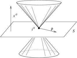
Figure 1: Spacetime close to spatial and null infinities: to the left the standard representation of spatial infinity as a point $i^{0}$; to the right the representation where spatial infinity is enviewed as a cylinder.

Most of the discussion here presented will be concerned with the extension $\mbox{\SYM M}_{\Theta}$ of Minkowski spacetime produced by the conformal factor $\Theta=\rho(1-\tau^{2})$. Using the null geodesics discussed in the previous paragraph one can construct an adapted null (NP) tetrad such that the real vector $l$ is tangent along the incoming null geodesics, and the vector $n$ points along the outgoing null geodesics . The complex vectors $m$ and $\overline{m}$ are then usually chosen so that they span the tangent space of the two dimensional spheres $S_{\rho^{\prime},\tau^{\prime}}=\{\rho=\rho^{\prime},\tau=\tau^{\prime}\}$, with $\rho^{\prime}$, $\tau^{\prime}$ given. This construction has the problem that $m$ should vanish at least in a point on $S_{\rho^{\prime},\tau^{\prime}}$. For technical reasons it will be therefore convenient to coordinatise the 2-spheres $S_{\rho,\tau}$ by means of unitary representations of $SU(2,\mbox{\SYM C})$. This can be done as the unit sphere $S^{2}$ can be identified with $SU(2,\mbox{\SYM C})/U(1)$ which is obtained from $S^{3}\simeq SU(2,\mbox{\SYM C})$ via the Hopf map. Any real analytic function $f$ on $SU(2,\mbox{\SYM C})$ admits an expansion of the form,

$$f=\sum_{m=0}^{\infty}\sum_{j=0}^{m}\sum_{k=0}^{m}f_{m,k,j}T_{m\phantom{k}j}^{\phantom{m}k},$$

with complex coefficients $f_{m,k,j}$. The functions $T_{m\phantom{k}j}^{\phantom{m}k}$ $m=0,1,2,\ldots$, $j,k=0,\ldots,m$ can be related to the spherical harmonics $Y_{l,n}$ FriKan00 . The function $f$ will be said to have spin-weight $s$ if its expansion in terms of the $T_{m\phantom{k}j}^{\phantom{m}k}$ functions is of the form,

$$f=\sum_{q=|s|}^{\infty}\sum_{k=0}^{2q}f_{q,k}T_{2q\phantom{k}q-s}^{\phantom{2q}k}.$$

Important for later discussion will be the fact that any $C^{\infty}$ function $\phi=\phi(\rho,t)$ on $\mbox{\SYM R}_{0}^{+}\times SU(2,\mbox{\SYM C})$ such that for fixed $\rho$ it is of spin-weight $s$, with $s$ independent of $\rho$ has a normal expansion of the form,

$$\phi=\sum_{p\geq|s|}\sum_{q=|s|}^{p}\sum_{k=0}^{2q}\phi_{p;q,k}T_{2q\phantom{k}q-s}^{\phantom{2q}k}\rho^{p},$$

with $\phi_{p;q,k}$ complex. This last result will be extensively used. For further details on the $T_{m\phantom{k}j}^{\phantom{m}k}$ functions, the reader is referred to Fri86a .

3 Linearised gravity in the F-gauge

We will describe the linearised gravitational by means of a spin-2 zero-rest-mass field $\phi_{abcd}$ satisfying,

$$\nabla^{aa^{\prime}}\phi_{abcd}=0.$$

Using the null tetrad described in the previous section, one can recover the $(D,\overline{\delta})$ and $(\Delta,\delta)$ equations of the NP formalism (see e.g. NewPen62 ; PenRin84 ) :

$$(1+\tau)\partial_{\tau}\phi_{n}-\rho\partial_{\rho}\phi_{n}+X_{+}\phi_{n+1}=(n-2)\phi_{n},$$ (3)

$$(1-\tau)\partial_{\tau}\phi_{n+1}+\rho\partial_{\rho}\phi_{n+1}+X_{-}\phi_{n}=(n-1)\phi_{n+1}$$ (4)

where $n=0,1,2,3$. The coefficients $\phi_{n}$ can be shown to have spin-weight $2-n$. The operators $X_{+}$ and $X_{-}$ are complex linear combinations of left invariant vector fields on $SU(2,\mbox{\SYM C})$, and can be related to the $\eth$ and $\overline{\eth}$ operators of Newman & Penrose FriKan00 . The NP equations (3) and (4) imply a set of five propagation equations,

$$(1+\tau)\partial_{\tau}\phi_{0}-\rho\partial_{\rho}\phi_{0}+X_{+}\phi_{1}=-2\phi_{0},$$ (5)

$$\partial_{\tau}\phi_{1}+\textstyle\frac{1}{2}X_{-}\phi_{0}+\frac{1}{2}X_{+}\phi_{2}=-\phi_{1},$$ (6)

$$\partial_{\tau}\phi_{2}+\textstyle\frac{1}{2}X_{-}\phi_{1}+\frac{1}{2}X_{+}\phi_{3}=0,$$ (7)

$$\partial_{\tau}\phi_{3}+\textstyle\frac{1}{2}X_{-}\phi_{2}+\frac{1}{2}X_{+}\phi_{4}=\phi_{3},$$ (8)

$$(1-\tau)\partial_{\tau}\phi_{4}+\rho\partial_{\rho}\phi_{4}+X_{-}\phi_{3}=2\phi_{4},$$ (9)

and a set of three constraint equations,

$$\tau\partial_{\tau}\phi_{1}-\rho\partial_{\rho}\phi_{1}+\textstyle\frac{1}{2}X_{+}\phi_{2}-\frac{1}{2}X_{-}\phi_{0}=0,$$ (10)

$$\tau\partial_{\tau}\phi_{2}-\rho\partial_{\rho}\phi_{2}+\textstyle\frac{1}{2}X_{+}\phi_{3}-\frac{1}{2}X_{-}\phi_{1}=0,$$ (11)

$$\tau\partial_{\tau}\phi_{3}-\rho\partial_{\rho}\phi_{3}+\textstyle\frac{1}{2}X_{+}\phi_{4}-\frac{1}{2}X_{-}\phi_{2}=0.$$ (12)

This latter set of equations gives rise to equations on the initial hypersurface $S=\{\tau=0\}$ which correspond to the constraints coming from the linearised Bianchi identities.

Using the equations (5)-(9) one obtains a symmetric hyperbolic system CouHil62 ; Joh91 by simply multiplying (6)-(8) by a factor of 2. The resulting system is of the form:

$$A^{0}\partial_{\tau}\Phi+A^{1}\partial_{\rho}\Phi+A^{+}X_{+}\Phi+A^{-}X_{-}\Phi+B\Phi=0,$$ (13)

where $A^{\mu}$ $\mu=0,1,2,3$ and $B$ are $5\times 5$ matrices. It can be more concisely written in the form of $(A^{\mu})_{\alpha\beta}\partial_{\mu}\phi_{\beta}+B_{\alpha}=0$. Crucial for our discussion will be to realize that the matrix $A^{0}=\mbox{diag}(1+\tau,2,2,2,1-\tau)$ looses rank at $\tau=\pm 1$. This degeneracy will be the source of most our problems as this fact precludes the direct use of the standard theory of symmetric hyperbolic systems.

Let Q be the $5\times 5$ matrix with components given by,

$$(Q)_{\alpha\beta}=(A^{\mu})_{\alpha\beta}\partial_{\mu}\phi.$$

Then the characteristics of the system (13) are the hypersurfaces $\phi=k$, with $k$ a real constant, and such that the scalar field $\phi$ satisfies,

$$\det Q=0.$$

It can be readily checked that the hypersurfaces $u=k$ and $v=k^{\prime}$, with $u$ and $v$ defined as in the preceeding section are characteristics of the symmetric hyperbolic system (13). In particular, the hypersurfaces defined by $v=0$ and $u=0$ with $\rho\neq 0$ correspond to ${I}^{+}$ and ${I}^{-}$ respectively. Hence, ${I}^{+}$ and ${I}^{-}$ are both characteristic hypersurfaces of the system (13). The evaluation of the NP equations (4) on ${I}^{+}$ gives rise to transport equations which enable us to calculate the value of the components $\phi_{1},\ldots,\phi_{4}$ on ${I}^{+}$ from a knowledge of the radiation field $\phi_{0}$ on ${I}^{+}$. Similarly, using equations (3) one obtains a corresponding set of transport equations on ${I}^{-}$ by means of which it is possible to calculate the values of $\phi_{0},\ldots,\phi_{3}$ from a knowledge of $\phi_{4}$ on ${I}^{-}$.

A further look to the system (13) reveals that at $\rho=0$ the whole system reduces to transport equations which enable us to calculate the value of $\phi_{n}$ ($n=0,\ldots,4$) from their value at the initial hypersurface $S$. Hence, we say that $I$ is a total characteristic of (13). As a consequence, no boundary data can be prescribed on $I$.

3.1 Initial data for linearised gravity

That the spin 2 zero-rest-mass field $\phi_{abcd}$ can be used to describe the linearised gravitational field can be seen as follows. Consider a family $\widetilde{g}_{\mu\nu}(\lambda)$ of spacetimes depending in a $C^{1}$ fashion on the parameter $\lambda$, and such that at $\lambda=0$ one obtains Minkowski spacetime. Therefore,

$$\widetilde{g}_{\mu\nu}=\widetilde{\eta}_{\mu\nu}+\lambda\widetilde{h}_{\mu\nu}+\mathcal{O}(\lambda^{2}).$$

The symmetric rank 2 tensor $\widetilde{h}_{\mu\nu}$ describes the first order deviation from flatness of the metric $\widetilde{g}_{\mu\nu}$. The computation of the curvature to first order in $\lambda$ yields PenRin84 ,

$$\widetilde{K}_{\mu\nu\lambda\rho}=2\widetilde{\nabla}_{[\mu}\widetilde{\nabla}_{|[\nu}\widetilde{h}_{\lambda]|\rho]},$$

where $\widetilde{\nabla}_{\mu}$ is the covariant derivative of the flat spacetime. Then the linearised field equations take the form:

$$\widetilde{K}_{\mu\nu\lambda}^{\phantom{\mu\nu\lambda}\rho}=0.$$ (14)

The tensor $\widetilde{K}_{\mu\nu\lambda\rho}$ is trace-free and possesses the same symmetries of the Riemann tensor. It can be described in spinorial language by a totally symmetric spinor $\widetilde{\phi}_{abcd}$ satisfying the spin-2 zero-rest-mass field equation:

$$\widetilde{\nabla}^{aa^{\prime}}\widetilde{\phi}_{abcd}=0.$$ (15)

Equation (15) is a sufficient condition for the tensor $\widetilde{K}_{\mu\nu\lambda\rho}$ to be derivable (locally) from some symmetric tensor $\widetilde{h}_{\mu\nu}$ SacBer58 . If the spinorial field $\widetilde{\phi}_{abcd}$ is set to transform as $\phi_{abcd}=\Omega^{-1}\widetilde{\phi}_{abcd}$ then the equation (15) is conformally covariant.

Let us assume that the family of metrics $\widetilde{g}_{\mu\nu}(\lambda)$ arise from the Einstein evolution of a corresponding 1-parameter family of asymptotically flat, time symmetric initial data given by the 3-dimensional metric,

$${}^{(3)}\widetilde{g}_{\alpha\beta}=\widetilde{\delta}_{\alpha\beta}+\lambda\;\;{}^{(3)}\widetilde{h}_{\alpha\beta}+\mathcal{O}(\lambda^{2}).$$

It will be assumed that ${}^{(3)}\widetilde{g}_{\alpha\beta}$ satisfies the time symmetric vacuum constraint equations. Then, the symmetric tensor ${}^{(3)}\widetilde{h}_{\alpha\beta}$ is a solution of the corresponding linearised vacuum constraint equations. In the present discussion we will consider 1-parameter families of 3-metrics ${}^{(3)}\widetilde{g}_{\alpha\beta}$ such that their suitably conformally rescaled counterparts ${}^{(3)}{g}_{\alpha\beta}$ extend analytically near $i$, the infinity of the initial Cauchy hypersurface. For conceptual reasons it is convenient to distinguish $i$ from $i^{0}$, the spatial infinity of the whole spacetime. It can be proved Fri98a that under this assumption the components of the conformally rescaled Weyl spinor of the family of metrics $g_{\mu\nu}(\lambda)$ in the unphysical spacetime evaluated on the initial hypersurface $S$ are of the form,

$$\psi_{n}(\lambda)|_{S}=\sum_{p=|2-n|}^{\infty}\psi_{n}^{p}(\lambda)|_{S}\rho^{n},$$

where

$$\psi_{n}^{p}(\lambda)|_{S}=\sum_{q=|2-n|}^{p}\;\sum_{k=0}^{2q}c_{n,p;q,k}(\lambda)T_{2q\phantom{k}q-2+n}^{\phantom{2q}k}$$

with complex coefficients $c_{n,p;q,k}$ $n=0,1,2,3$. Now, upon linearisation one obtains a similar behaviour for the components of the spinorial field $\phi_{abcd}$. Namely,

$$\phi_{n}|_{\tau=0}=\sum_{p=|2-n|}^{\infty}\phi_{n}^{p}|_{\tau=0}\rho^{n},$$ (16)

where

$$\phi_{n}^{p}|_{\tau=0}=\sum_{q=|2-n|}^{p}\sum_{k=0}^{2q}d_{n,p;q,k}T_{2q\phantom{k}q-2+n}^{\phantom{2q}k}.$$

The components of the Weyl spinor $\psi_{n}$ satisfy the constraints coming from the Bianchi identities. Hence, the components $\phi_{n}$ satisfy automatically their linearised version —equations (10)-(12) on $S=\{\tau=0\}$.

Later considerations will make use of a particular spinorial object: the Cotton spinor (sometimes also called Bach spinor). The Cotton spinor $B_{abcd}$ is the 3-dimensional analogue of the Weyl spinor Fri88 . It locally characterises conformally flat 3-metrics in the sense that it vanishes identically if and only if the 3-metric is locally conformally flat. One can construct its corresponding linearised version $b_{abcd}$. Linearisation around Minkowski yields the following expression,

$$b_{abcd}=2D_{e(a}\Omega\phi_{bcd)}^{\phantom{bcd)}e}+\Omega D_{e(a}\phi_{bcd)}^{\phantom{bcd)}e},$$

where $\Omega=\rho^{2}$ is the conformal factor of the 3-metric of the Minkowski initial data, and $D_{ab}$ its corresponding spinorial covariant derivative.

Inspired in a similar result by Friedrich we present now the following rather technical result. It will be of much use in later discussions.

Lemma 1

The coefficients $d_{j,p;p,k}$ of the spin-2 zero-rest-mass (16) field satisfy the antisymmetry condition

$$d_{0,p;p,k}|_{\tau=0}=-d_{4,p;p,k}|_{\tau=0},\qquad p=0,1,\ldots,\;\;k=0,\ldots 2p.$$ (17)

Furthermore,

$$d_{j,p;p,k}|_{\tau=0}=0,\qquad p=0,\ldots,s^{*},\;\;k=0,\dots,2p,\;\;j=0,\ldots,4.$$

if and only if

$$D_{(a_{q}b_{q}}\cdots D_{a_{1}b_{1}}b_{abcd)}(i)=0,\qquad q=0,\ldots,s^{*}.$$

The proof follows from direct linearisation of theorem 4.1 in Fri98a .

4 A regularity condition at spatial infinity

We now proceed to carry out an analysis of the transport equations one obtains upon evaluation of the field equations (5)-(9) and (10)-(12). Consider the equations (5)-(9) and (10)-(12). Differentiating them formally with respect to $\rho$ and evaluating at the cylinder at $\rho=0$ one gets:

$$(1+\tau)\partial_{\tau}\phi^{p}_{0}+X_{+}\phi_{1}^{p}-(p-2)\phi_{0}=0,$$ (18)

$$\partial_{\tau}\phi^{p}_{1}+\textstyle\frac{1}{2}(X_{-}\phi^{p}_{0}+X_{+}\phi^{p}_{2})+\phi_{1}=0,$$ (19)

$$\partial_{\tau}\phi^{p}_{2}+\textstyle\frac{1}{2}(X_{-}\phi^{p}_{1}+X_{+}\phi^{p}_{3})=0,$$ (20)

$$\partial_{\tau}\phi^{p}_{3}+\textstyle\frac{1}{2}(X_{-}\phi^{p}_{2}+X_{+}\phi^{p}_{4})-\phi^{p}_{3}=0,$$ (21)

$$(1-\tau)\partial_{\tau}\phi^{p}_{4}+X_{-}\phi^{p}_{3}+(p-2)\phi^{p}_{4}=0,$$ (22)

and

$$\tau\partial_{\tau}\phi^{p}_{1}+\textstyle\frac{1}{2}(X_{+}\phi^{p}_{2}-X_{-}\phi^{p}_{0})-p\phi_{1}^{p}=0,$$ (23)

$$\tau\partial_{\tau}\phi^{p}_{2}+\textstyle\frac{1}{2}(X_{+}\phi^{p}_{3}-X_{-}\phi^{p}_{1})-p\phi_{2}^{p}=0,$$ (24)

$$\tau\partial_{\tau}\phi^{p}_{3}+\textstyle\frac{1}{2}(X_{+}\phi^{p}_{4}-X_{-}\phi^{p}_{2})-p\phi_{3}^{p}=0,$$ (25)

where we have set $\phi^{p}_{n}=\partial_{\rho}^{(p)}\phi_{n}|_{\rho=0}$. One can expand these coefficients using the functions $T_{k\phantom{l}m}^{\phantom{k}l}$ in the form:

$$\phi^{p}_{n}=\sum_{q=|2-n|}^{p}\sum_{k=0}^{2q}a_{n,p;q,k}T_{2q\phantom{k}q-2+n}^{\phantom{2q}k}.$$ (26)

The coefficients $a_{n,p;q,k}$ are, in principle, complex functions of $\tau$. Using these expansions and the equations (19)-(21) and (23)-(25), one can calculate the coefficients $a_{1,p;q,k}$, $a_{2,p;q,k}$, $a_{3,p;q,k}$ from a knowledge of the $a_{0,p;q,k}$ and $a_{4,p;q,k}$ via a first order algebraic linear system. Some more algebra leads to,

$$\!\!\!\!\!\!\!\!\!\!\!\!(1-\tau^{2})\ddot{a}_{0,p;q,k}+(4+2(p-1)\tau)\dot{a}_{0,p;q,k}+(q+p)(q-p+1)a_{0,p;q,k}=0,$$ (27)

$$\!\!\!\!\!\!\!\!\!\!\!\!(1-\tau^{2})\ddot{a}_{4,p;q,k}+(-4+2(p-1)\tau)\dot{a}_{4,p;q,k}+(q+p)(q-p+1)a_{4,p;q,k}=0,$$ (28)

for $p\geq 2$, $2\leq q\leq p$, the overdot denoting differentiation with respect to $\tau$. The equations (27) and (28) are examples of Jacobi equations. A canonical parametrisation for this class of ordinary differential equations is:

$$D_{(n,\alpha,\beta)}a\equiv(1-\tau^{2})a^{\prime\prime}+\{\beta-\alpha-(\alpha+\beta+2\tau)\}a^{\prime}+n(n+\alpha+\beta+1)a=0.$$ (29)

In our case the parameters are given by: $\alpha_{0}=\beta_{4}=-p-2$, $\beta_{0}=\alpha_{4}=-p+2$, $n_{1}=p+q$, and $n_{2}=p-q-1$. Regular solutions for equations (27) and (28) exist for $q\neq p$, and are given quite concisely in terms of Jacobi polynomials Sze78 . Namely,

$$a_{0,p;q,k}=C_{1}P_{p-q-1}^{(-p-2,-p+2)}(\tau)+C_{2}\left(\frac{1-\tau}{2}\right)^{p+2}P_{q-2}^{(p+2,-p+2)}(\tau),$$ (30)

$$a_{4,p;q,k}=D_{1}P_{p-q-1}^{(-p+2,-p-2)}(\tau)+D_{2}\left(\frac{1-\tau}{2}\right)^{p-2}P_{q+2}^{(p-2,-p-2)}(\tau),$$ (31)

where $C_{1}$, $C_{2}$, $D_{1}$ and $D_{2}$ are constants which can be determined from the initial data at $\tau=0$. In the case $q=p$, the use of some identities of the Jacobi equation (29) leads to:

$$\!\!\!\!\!\!\!\!\!\!\!\!\!a_{0,p;p,k}=\left(\frac{1-\tau}{2}\right)^{p+2}\left(\frac{1+\tau}{2}\right)^{p-2}\left(E_{0}+E_{1}\int_{0}^{\tau}\frac{ds}{(1+s)^{p-1}(1-s)^{p+3}}\right)$$ (32)

$$\!\!\!\!\!\!\!\!\!\!\!\!\!a_{4,p;p,k}=\left(\frac{1-\tau}{2}\right)^{p-2}\left(\frac{1+\tau}{2}\right)^{p+2}\left(F_{0}+F_{1}\int_{0}^{\tau}\frac{ds}{(1+s)^{p+3}(1-s)^{p-1}}\right).$$ (33)

The use of Taylor expansions in the integrals shows that they give rise to logarithmic terms. More precisely, recalling that:

$$\int_{0}^{\tau}\frac{ds}{(1\pm s)^{p-1}(1\mp s)^{p+3}}=A_{*}\ln(1-\tau)+\frac{A_{p\pm 2}}{(1-\tau)^{p\pm 2}}+\cdots+\frac{A_{1}}{(1-\tau)}+A_{0}$$

$$\phantom{\int_{0}^{\tau}\frac{ds}{(1+s)^{p-1}(1-s)^{p+3}}=}+B_{*}\ln(1+\tau)+\frac{B_{p\mp 2}}{(1+\tau)^{p\mp 2}}+\cdots+\frac{B_{1}}{(1+\tau)},$$

where the $A$’s and $B$’s are some constants. From the latter expansions one can conclude that the only non-regular coefficients in $a_{0,p;q,k}$ and $a_{4,p;q,k}$ in the $q=p$ case are of logarithmic nature. Analytic solutions arise if and only if $a_{0,p;p,m}(0)=a_{4,p;p,m}(0)$. That is only the case if the constants $E_{1}$ and $F_{1}$ in equations (32) and (33) are both zero. Now, using the antisymmetry condition (17) of lemma 1 one learns that in fact $a_{0,p;p,m}(0)=a_{4,p;p,m}(0)=0$. It is not hard to see that if this is the case, then $a_{j,p;p,m}(0)=0$ for $j=0,\dots,4$. Finally, using the second part of lemma 1 one can relate this behaviour of the initial data to the vanishing of the linearised Cotton tensor and its symmetrised derivatives on $i$. The results of the previous discussion are summarised in the following theorem.

Theorem 4.1

The solutions of the transport equations on $I$ corresponding to the system (5)-(9) and (10)-(12) extend analytically to $I^{\pm}$ if and only if the regularity condition

$$D_{(a_{s}b_{s}\cdots}D_{a_{1}b_{1}}b_{abcd)}(i)=0,\quad s=0,1,\dots\;\;,$$ (34)

holds.

A peculiarity of the logarithms appearing in the solutions of the transport equations is that they only occur at the highest spherical harmonics sector at each order. This will be of importance later when discussion the asymptotic expansions of the field $\phi_{abcd}$ close to ${I}^{+}$.

The aforediscussed solutions of the transport equations allow us to obtain normal expansions of the form,

$$\phi_{n}=\sum_{p\geq|2-n|}\phi_{n}^{p}\rho^{p},$$ (35)

with the coefficients $\phi_{n}^{p}$ given by (26). Now, it is of interest to see how the form of these normal expansions and the regularity condition (34) reflect on the structure of the asymptotic expansions close to null infinity. In order to do this, one has essentially to reshuffle the normal expansions. So far, our discussion has applied to both future and past null infinities. The forthcoming analysis will without loss of generality be focused on ${I}^{+}$. Nevertheless, a totally analogous treatment can be performed for ${I}^{-}$.

Putting together the results from the analysis of the transport equations (18)-(22) and (23)-(25) one obtains normal expansions for the coefficients $\phi_{0}$ and $\phi_{4}$ which are of the form,

$$\phi_{0}=\sum_{p=2}\left(S[0](1-\tau)+a_{*}^{p}\ln(1-\tau)P[p+2,2p](1-\tau)\right)\rho^{p},$$

$$\phi_{4}=\sum_{p=2}\left(S[0](1-\tau)+b_{*}^{p}\ln(1-\tau)P[p-2,2p](1-\tau)\right)\rho^{p}.$$

By $S[n](x)$ it will be understood a generic infinite series in $x$ starting with $x^{n}$. Similarly, $P[n_{1},n_{2}](x)$ denotes generic polynomials in $x$ of order $n_{2}$ and whose lowest order term is $x^{n_{1}}$. The coefficients $a_{*}^{p}$, $b_{*}^{p}$ and those in the series/polynomials are given in terms of the functions $T_{m\phantom{k}j}^{\phantom{m}k}$. Matters of convergence of the normal expansions will be addressed in the next section. Now, a careful reshuffling in order to obtain expansions in $(1-\tau)$ reveal that,

$$\!\!\!\!\!\!\!\phi_{0}=\sum_{p=0}^{3}S[2](\rho)(1-\tau)^{p}+\!\!\sum_{p\geq 4}\left(S[2](\rho)+\!\!\!\!\sum_{s=[t/2]}^{t-2}a^{s}_{*}\rho^{s}\ln(1-\tau)\right)(1-\tau)^{p},$$

$$\!\!\!\!\!\!\!\phi_{4}=\sum_{p\geq 0}\left(S[2](\rho)+\!\!\!\!\sum_{s=[t/2]}^{t+2}b^{s}_{*}\rho^{s}\ln(1-\tau)\right)(1-\tau)^{p},$$

where $[t/2]=t/2$ if $t$ is even, and $[t/2]=(t+1)/2$ if $t$ is odd. Notice that the component $\phi_{4}$ happens to be the most singular one of the field. If the regularity condition (34) is satisfied up to $s=s_{*}$, then it is not hard to see that,

$$\phi_{4}=\sum_{k=0}^{s_{*}+1}\ c_{k}(1-\tau)^{k}+d_{s_{*}+1}(1-\tau)^{s_{*}+1}\ln(1-\tau)+\cdots,$$ (36)

where the coefficients $c_{k}$ are $C^{\infty}$ functions of $\rho$ and the angular variables, and

$$d_{s_{*}+1}=\rho^{s_{*}+3}\sum_{m=0}^{2s_{*}+6}D_{s_{*}+1,m}T_{2s_{*}+6\phantom{m}s_{*}+5}^{\phantom{2s_{*}+6}m},$$ (37)

with $D_{s_{*}+1,m}$ complex constants. Thus, the logarithmic term in the expansion has only dependence in the highest spherical harmonic sector possible at this order, i.e. $q=s_{*}+3$. Finally, if the regularity condition holds also for $s=s_{*}+1$ then $d_{s_{*}+1}=0$.

5 Polyhomogeneous expansions

5.1 A substraction argument

So far, nothing has been said about the convergence of the normal expansions (35) calculated in the previous section. We will now discuss how this can be done. As before, we write $\Phi=(\phi_{0},\phi_{1},\phi_{2},\phi_{3},\phi_{4})$. Let,

$$\Phi_{N}=\sum_{p=0}^{N}\frac{1}{p!}\Phi^{p}\rho^{p},$$

be the $N$ order partial sum. The linear field equations (5)-(9) and (10)-(12) are such that $\Phi_{N}$ itself happens to be a solution of the field equations with truncated (to order $N$) initial data. The regularity of $\Phi_{N}$ will depend on whether the initial data satisfies the regularity condition (34) to a given order or not. For example, if the condition is satisfied up to $s=N$, then no $\ln(1-\tau)$ term will be present in the coefficients $\Phi^{p}$, and thus $\Phi_{N}$ will be $C^{\infty}$. How could one estimate the rest? Recall that the symmetric hyperbolic system derived from equations (5)-(9) breaks down precisely at $\tau=1$. This is rather unfortunate, as we are mainly interested in observing the behaviour of the solutions on null infinity.

Bounds for the rest can be obtained by considering the conformal extension of Minkowski, $\mbox{\SYM M}_{\Xi}$, in which spatial infinity is represented by a point $i^{0}$. The spin 2 zero-rest-mass field equations given in spherical coordinates are formally singular at $\rho=0$ in this representation. Therefore, we resort to Cartesian coordinates $(x^{\mu})$. In this way, the propagation equations read,

$$\partial_{0}\widehat{\phi}_{0}-\partial_{3}\widehat{\phi}_{0}+\partial_{1}\widehat{\phi}_{1}+i\partial_{2}\widehat{\phi}_{1}=0,$$

$$2\partial_{0}\widehat{\phi}_{1}+\partial_{1}\widehat{\phi}_{2}+\partial_{1}\widehat{\phi}_{0}+i\partial_{2}\widehat{\phi}_{2}-i\partial_{2}\widehat{\phi}_{0}=0,$$

$$2\partial_{0}\widehat{\phi}_{2}+\partial_{1}\widehat{\phi}_{3}+\partial_{1}\widehat{\phi}_{1}+i\partial_{2}\widehat{\phi}_{3}-i\partial_{2}\widehat{\phi}_{1}=0,$$

$$2\partial_{0}\widehat{\phi}_{3}+\partial_{1}\widehat{\phi}_{4}+\partial_{1}\widehat{\phi}_{2}+i\partial_{2}\widehat{\phi}_{4}-i\partial_{2}\widehat{\phi}_{2}=0,$$

$$\partial_{0}\widehat{\phi}_{4}+\partial_{3}\widehat{\phi}_{4}+\partial_{1}\widehat{\phi}_{3}-i\partial_{2}\widehat{\phi}_{3}=0,$$

while the constraint equations are given by,

$$2\partial_{3}\widehat{\phi}_{1}+\partial_{1}\widehat{\phi}_{0}-\partial_{1}\widehat{\phi}_{2}-i\partial_{2}\widehat{\phi}_{0}-i\partial_{2}\widehat{\phi}_{2}=0,$$

$$2\partial_{3}\widehat{\phi}_{2}+\partial_{1}\widehat{\phi}_{1}-\partial_{1}\widehat{\phi}_{3}-i\partial_{2}\widehat{\phi}_{1}-i\partial_{2}\widehat{\phi}_{3}=0,$$

$$2\partial_{3}\widehat{\phi}_{3}+\partial_{1}\widehat{\phi}_{2}-\partial_{1}\widehat{\phi}_{4}-i\partial_{2}\widehat{\phi}_{2}-i\partial_{2}\widehat{\phi}_{4}=0.$$

The components of the linearised Weyl tensor rescale as follows: $\widehat{\phi}_{n}=\rho^{-1-n}\phi_{n}$, $n=0,\ldots,4$, where $\rho^{2}=(x^{1})^{2}+(x^{2})^{2}+(x^{3})^{2}$. Thus, the smooth data in $\mbox{\SYM M}_{\Theta}$ discussed in §3.1, and such that $\phi_{0}=\mathcal{O}(\rho^{2})$, $\phi_{1}=\mathcal{O}(\rho)$, $\phi_{2}=\mathcal{O}(1)$, $\phi_{3}=\mathcal{O}(\rho)$ and $\phi_{4}=\mathcal{O}(\rho^{2})$, becomes singular in the $\mbox{\SYM M}_{\Xi}$ picture at $i$ (i.e. $\rho=0$). However, if one provides initial data with sufficiently fast decay at $i^{0}$ then one can obtain energy estimates of the form,

$$\|\widehat{\Phi}\|^{2}_{L^{2}(\mho)}\leq C\|\widehat{\Phi}\|^{2}_{L^{2}(\Sigma_{1})},$$ (38)

where $\|\phantom{X}\|^{2}_{L^{2}(\mho)}$ and $\|\phantom{X}\|^{2}_{L^{2}(\Sigma_{1})}$ denote the $L^{2}$ norms over the region $\mho$ and the hypersurface $\Sigma_{1}$ respectively. Higher order estimates for the derivatives can be similarly obtained. The domain $\mho$ is as shown in figure (2). Notice how in this way one can obtain estimates that go up to ${I}^{+}$ —and through it.

Figure 2: The region of integration used to obtain the energy estimate (38). The first picture shows the domain of integration in the representation where spatial infinity is enviewed as a cylinder, and the second in the in the standard representation of spatial infinity as a point. Note that $\Sigma_{2}$ which seems to be an extended 2 dimensional surface is in fact a point: $i^{0}$. The surface $\Sigma_{3}$ is spacelike and almost flat, and may reach and go through null infinity.

In this spirit consider,

$$\widehat{X}=\widehat{\Phi}-\widehat{\Phi}_{N}.$$

A close look to the rescaling rules will convince us that:

$$\widehat{X}|_{\tau=0}=\mathcal{O}(\rho^{N-5}).$$

It can be readily checked that such a decay implies $\widehat{X}|_{\tau=0}\in H^{N-4}(\Sigma_{1})$, where $H^{k}(\Sigma_{1})$ denotes the $k$-th Sobolev space over the domain $\Sigma_{1}$ . Standard theory of linear of symmetric hyperbolic systems (see for example Tay96 ) then guarantees the existence of $\widehat{X}$ such that $\widehat{X}\in C^{N-7}(\mho)$. Hence, we have estimated the rest of the partial sum $\Phi_{N}$. If one wants the solution to be of class $C^{k}(\mho)$, $k\in\mbox{\SYM N}$, then the previous discussion shows that one needs the regularity condition (34) to hold up to order $s=k+7$.

The disadvantage of this approach is that it is hard to extend for the case of quasilinear equations. Therefore, it will be of little use when we eventually try to address the full non-linear gravitational field. We need to devise something else.

5.2 An investigation of expansions close to null infinity

The analysis of the solutions of the transport equations on the the spatial infinity cylinder $I$ show that logarithmic divergences will generically arise at $I^{\pm}$ for smooth initial data of the sort considered in §3.1 unless the regularity condition (34) is satisfied. Accordingly, if the regularity condition is satisfied, then the solutions to the transport equations extend smoothly through $I^{+}$. This is a hint that the evolution of generic smooth initial data will be polyhomogeneous, i.e. its expansions will contain $\ln(1-\tau)$ terms. An analysis and a discussion of the properties of such spacetimes close to null infinity, including the existence of an intriguing set of conserved quantities analogous to the Newman-Penrose constants has been given in ChrMacSin95 ; Val98 ; Val99a ; Val99b ; Val00a . The regularity condition given in theorem 4.1 ensures that the solutions of the transport equations (18)-(22) and (23)-(25) extend analytically to $I^{\pm}$. Now, with the discussion on $I^{+}$ more or less settled, one would like to study the effects the degeneracy of the field equations on $I^{+}$ has one null infinity. In particular, one would like to know what do the logarithmic terms on $I^{+}$ imply on ${I}^{+}$. How do they propagate? In order to investigate this point, we resort to some ideas coming from the asymptotic characteristic initial value problem Fri81b ; Fri81a ; Kan96b . Consider a future oriented null hypersurface $\mathcal{N}_{0}$ intersecting ${I}^{+}$ at $\mathcal{Z}_{0}$. One can provide characteristic initial data in the following way: $\phi_{4}$ is prescribed on $\mathcal{N}_{0}$, $\phi_{0}$ on the portion of ${I}^{+}$ comprised between $\mathcal{Z}_{0}$ and $I^{+}$, and $\phi_{2}$ and $\phi_{1}$ on $\mathcal{Z}_{0}$. Theorems providing existence in a neighbourhood $\mho\subset J^{-}(\mathcal{Z}_{0})$ of $\mathcal{Z}_{0}$ for the conformal Einstein equations have been given in Fri81b ; Fri81a ; Kan96b . An existence theorem for polyhomogeneous Maxwell fields has been given in Val00 .

Figure 3: The asymptotic characteristic initial value problem close to spatial infinity.

Problems with the characteristic approach have mainly to do with the ample freedom one has in choosing the initial data on $\mathcal{N}_{0}$. As an added factor, the theorems by Friedrich and Kánnár given only local existence. This is somehow a problem, as one would like to take the field $\phi_{abcd}$ all along ${I}^{+}$ and evaluate at the set $I^{+}$, and then compare with the results obtained from the transport equations on $I$.

Inspired by the aforementioned characteristic approach, we will make use of the transport equations obtained on ${I}^{+}$ arising from the NP equations (4). In this way once the radiation field $\phi_{0}$ is provided, the remaining field components can be obtained essentially by a mere integration along the generators of null infinity. Expansions containing $\ln(1-\tau)$ terms appeared in the normal expansions (35). However, it is of interest to consider a more general type of situation in which terms of the form $\ln^{k}(1-\tau)$ can arise. So, we will assume that the components of the spin 2 zero-rest-mass field $\phi_{abcd}$ have asymptotic expansions near to ${I}^{+}$ of the form,

$$\phi_{n}=\sum_{i\geq 0}\sum_{j=0}^{N_{i}}\phi_{n}^{(i,j)}(1-\tau)^{i}\ln^{j}(1-\tau),$$ (39)

$=0,\ldots,4\;$, where the coefficients $\phi_{n}^{(i,j)}$ contain only $\rho$ and angular dependence. They are assumed to be smooth at least in $\{\tau=1,0<\rho\geq\rho_{0}\}$ for $\rho_{0}$ a given non-negative real number. Some calculus rules will be needed in order to manipulate the polyhomogeneous expansions (39).

Assumption. For the expansions (39), it will be assumed that,

$$\partial_{\tau}\phi_{n}=-\sum_{i\geq 1}\sum_{j=0}^{N_{i}}\left(i\ln^{j}(1-\tau)+j\ln^{j-1}(1-\tau)\right)\phi_{n}^{(i,j)}(1-\tau)^{i-1},$$ (40)

$$\partial_{\rho}\phi_{n}=\sum_{i\geq 0}\sum_{j=0}^{N_{i}}\phi_{n}^{(i,j)^{\prime}}(1-\tau)^{i}\ln^{j}(1-\tau),$$ (41)

$$X_{\pm}\phi_{n}=\sum_{i\geq 0}\sum_{j=0}^{N_{i}}X_{\pm}\phi_{n}^{(i,j)}(1-\tau)^{i}\ln^{j}(1-\tau),$$ (42)

hold, where ^′ denotes differentiation with respect to $\rho$.

The above calculus rules can be used together with the transport equations on ${I}^{+}$ to obtain equations for the coefficients $\phi_{n}^{(i,j)}$ in the Ansatz (39). At each order $(1-\tau)^{p}$ the solutions to these equations will be calculated. The conditions under which the coefficients $\phi_{n}^{(i,j)}$ can be pushed down to will then be investigated. The idea is then to compare the expansions obtained by means of this procedure with those arising from solving the transport equations on $I$. If an identification of the two different expansions is possible, then one can analyse the effect the regularity condition (34) has on the asymptotic expansions close to spatial infinity ${I}^{+}$. Now, if at each order $(1-\tau)^{p}$ it is assumed that no $\log^{k}(1-\tau)$ terms are present in the lower terms, then it is possible to implement an inductive argument. The results of our forthcoming argument are summarised in the following theorem.

Theorem 5.1

Let,

• the components of the spin 2 zero-rest-mass field $\phi_{abcd}$ have an evolution expansion of the form

  $$\phi_{n}=\sum_{i\geq 0}\sum_{j=0}^{N_{i}}\phi_{n}^{(i,j)}(1-\tau)^{i}\ln^{j}(1-\tau),$$

  $n=0,\dots,4$ with the coefficients $\phi_{n}^{(i,j)}$ at least $C^{1}$ in $\{\tau=1,0<\rho\leq\rho_{0}\}$ for $\rho_{0}$ a non-negative constant;

• the calculus rules (40)-(42) hold;

• $\phi_{0}^{(0,0)}$ (the radiation field) be $C^{\infty}$ in $\{\tau=1,0\leq\rho\leq\rho_{0}\}\subset{I}^{+}\cup I^{+}$;

• $\phi_{1}^{(0,0)}$ and $\phi_{3}^{(0,0)}$ be bounded in $\{\tau=1,0\leq\rho\leq\rho_{0}\}$;

• the initial data $\phi_{n}|_{\tau=0}$, $n=0,\ldots,4$, be obtained by linearisation around flat space of asymptotically flat time symmetric initial data satisfying the Einstein vacuum constraints, and analytic in a neighbourhood of $i$;

• furthermore, the initial data satisfy the regularity condition

  $$D_{(a_{s}b_{s}}\cdots D_{a_{1}b_{1}}b_{abcd)}(i)=0\quad s=0,1,\dots;$$

• $\partial_{\rho}^{(k)}\phi_{4}^{(i,0)}$ be continuous in $\{\tau=1,0\leq\rho\leq\rho_{0}\}$, for $k=0,\ldots,i+2$ (tangential smoothness).

Then the expansions of $\phi_{n}$ are in fact logarithm-free, that is,

$$\phi_{n}=\sum_{i\geq 0}\phi_{n}^{(k,0)}(1-\tau)^{k},$$

where the coefficients $\phi_{n}^{(i,0)}$ are $C^{\infty}$ in $\{\tau=1,0\leq\rho\leq\rho_{0}\}$.

The base step $(1-\tau)^{0}$.

In agreement with the Ansatz (39) let the leading terms of the spin 2 zero-rest-mass field be of the form,

$$\phi_{n}=\sum_{j=0}^{N_{0}}\phi_{n}^{(0,j)}\ln^{j}(1-\tau)+\sum_{i\geq 1}\sum_{j=0}^{N_{i}}\phi_{n}^{(i,j)}(1-\tau)^{i}\ln^{j}(1-\tau),$$

with $n=0\ldots 4$. Direct substitution into equations (3) show that,

$$\phi_{0}^{(0,j)}=\phi_{1}^{(0,j)}=\phi_{2}^{(0,j)}=\phi_{3}^{(0,j)}=0,$$

for $j\geq 1$. The coefficients $\phi_{0}^{(0,0)}$, $\phi_{1}^{(0,0)}$, $\phi_{2}^{(0,0)}$ can be determined from the equations (4) $n=0,1,2$. The coefficients satisfy,

$$\rho\phi_{1}^{(0,0)\prime}+X_{-}\phi_{0}^{(0,0)}+\phi_{1}^{(0,0)}=0,$$ (43)

$$\rho\phi_{2}^{(0,0)\prime}+X_{-}\phi_{1}^{(0,0)}=0,$$ (44)

$$\rho\phi_{3}^{(0,0)\prime}+X_{-}\phi_{2}^{(0,0)}-\phi_{3}^{(0,0)}=0,$$ (45)

which can in principle be solved if the coefficient $\phi_{0}^{(0,0)}=\phi_{0}|_{{I}^{+}}$ (the radiation field) is given. It will be assumed that this is the case, and moreover, that it is $C^{\infty}$. Being $\phi_{0}^{(0,0)}$ smooth, one has that

$$\phi^{(0,0)}_{0}=\sum_{k\geq 2}f_{0,k}^{(0)}\rho^{k}=\sum_{k\geq 2}\left(\sum_{q=2}^{k}\sum_{m=0}^{2q}F^{(0)}_{0,k;q,m}T_{2q\phantom{m}q-2}^{\phantom{2q}m}\right)\rho^{k},$$ (46)

with $F^{(0)}_{0,k;q,m}$ complex constants. Using this expansion and equations (43)-(45) plus the further requirement of $\phi_{1}$ and $\phi_{3}$ to be smooth at $I^{+}$ one finds that,

$$\phi_{1}=\mathcal{O}(\rho^{2}),\quad\phi_{2}=\mathcal{O}(1),\quad\phi_{3}=\mathcal{O}(\rho).$$ (47)

The substitution of the Ansatz for the time development in equation (4) $n=3$, yields as a result the following hierarchy:

$$-2\phi_{4}^{(0,N_{0})}+\rho\phi_{4}^{(0,N_{0})\prime}=0,$$

$$-2\phi_{4}^{(0,N_{0}-1)}-\phi_{4}^{(0,N_{0})}+\rho\phi_{4}^{(0,N_{0}-1)\prime}=0,$$

$$\;\;\;\;\;\;\;\vdots$$

$$-2\phi_{4}^{(0,0)}-\phi_{4}^{(0,1)}+\rho\phi_{4}^{(0,0)\prime}+X_{-}\phi_{3}^{(0,0)}=0.$$

It can be solved from top to bottom, yielding:

$$\phi_{4}^{(0,N_{0})}=\widehat{\phi}_{4}^{(0,N_{0})}\rho^{2},$$ (48)

$$\phi_{4}^{(0,N_{0}-1)}=\widehat{\phi}_{4}^{(0,N_{0}-1)}\rho^{2}+\widehat{\phi}_{4}^{(0,N_{0})}\rho^{2}\ln\rho,$$ (49)

$$\phantom{\phi_{4}^{(0,N_{0}-1)}=}\vdots$$ (50)

$$\phi_{4}^{(0,0)}=\left[\frac{1}{N_{0}!}\widehat{\phi}_{4}^{(0,N_{0})}\rho^{2}\ln^{N_{0}}\rho+\cdots+\widehat{\phi}_{4}^{(0,0)}\rho^{2}\right]-\rho^{2}\int X_{-}\phi_{3}^{(0,0)}\rho^{-3}d\rho$$ (51)

where the hatted quantities denote functions which appear during the integration and thus, contain only angular dependence. The coefficients $\phi_{4}^{(0,j)}$ can be then “pushed down” to $I^{+}$, but not in general in such a way that they are smooth at $I^{+}$. The presence of terms of the form $\ln^{k}(1-\tau)$ in the Ansatz for the evolution yields as a result the presence of $\ln^{N_{0}-k}\rho$ terms in the corresponding expansions. This is an indication that if $\ln\rho$ terms are present in the initial data then these will propagate in the evolution via some particular $\ln^{k}(1-\tau)$ terms. Logarithmic terms of the form $\ln^{j}\rho$ do not appear in the normal expansions (35). Thus, in order to be able of performing an identification of the expansions on ${I}^{+}$ and $I$ some degree of tangential smoothness at $I^{+}$ will be assumed. A close look to formulae (51) shows that one needs $\phi_{4}^{(0,0)}$ to have two continuous $\rho$-derivatives at $I^{+}$. We will denote this by $\phi_{4}^{(0,0)}\in C^{2}_{\rho}(I^{+})$. This requirement now implies that $\widehat{\phi}_{4}^{(0,j)}=0$ for $j\geq 2$, and thus also $\phi_{4}^{(0,j)}=0$ for $j\geq 2$. Note that the “integration constant” $\widehat{\phi}_{4}^{(0,1)}$ does not need to vanish as the $\rho^{2}\ln\rho$ term in $\phi_{4}^{(0,0)}$ may be canceled with a similar one coming from $\rho^{2}\int X_{-}\phi_{3}^{(0,0)}\rho^{-3}d\rho$. Indeed, the integral $\rho^{2}\int X_{-}\phi_{3}^{(0,0)}\rho^{-3}d\rho$ produces a term of the form $\rho^{2}\ln\rho$ from the $\rho^{2}$ term in $\phi_{3}^{(0,0)}$. As discussed previously,

$$\phi_{3}^{(0,0)}=\sum_{k\geq 1}f_{3,k}^{(0)}\rho^{k},$$ (52)

where the coefficients $f^{(0)}_{3,k}$ are calculated from the $f^{(0)}_{0,k}$ of equation (46) by means of equations (43)-(45). Setting $\widehat{\phi}_{4}^{(0,1)}=X_{-}f_{3,2}^{(0)}$ in accordance with our previous discussion one finds that,

$$\phi_{4}^{(0,1)}=X_{-}f_{3,2}^{(0)}\rho^{2},$$ (53)

$$\phi_{4}^{(0,0)}=\widehat{\phi}_{4}^{(0,0)}\rho^{2}-\sum_{\begin{subarray}{c}k\geq 1\\ k\neq 2\end{subarray}}\frac{X_{-}f_{3,k}^{(0)}}{k-2}\rho^{k}.$$ (54)

One expects to be able to deduce the required degree of tangential smoothness form the smoothness properties of the initial data.

Finally, one is now in the position of performing an identification of the expansions obtained from the analysis of the transport equations on the cylinder, and those obtained from the transport equations at ${I}^{+}$. As discussed, both expansions contain $\ln(1-\tau)$ terms. However, the $\ln(1-\tau)$’s in the normal expansions appear only at the highest spherical sector at each order. So do those in our asymptotic expansions: from equation (52) one has,

$$f_{3,2}^{(0)}=\sum^{2}_{q=1}\sum_{m=0}^{2q}F^{(0)}_{3,2;q,m}T_{2q\;\;\;q+1}^{\;\;\;m}.$$

And hence,

$$X_{-}f_{3,2}^{(0)}=-\sum_{q=1}^{2}\sum_{m=0}^{2q}F^{(0)}_{3,2;q,m}\beta_{2q,q+2}T_{2q\;\;\;q+2}^{\;\;\;m},$$

with $\beta_{2q,q+2}=\sqrt{(q+2)(q-1)}$. Thus, $X_{-}$ cancels the sector given by $q=1$, and as a consequence the only non-zero sector in (53) is $q=2$. It is noticed by passing that $X_{-}\phi_{4}^{(0,1)}=0$ whence it follows that (tangential smoothness assumed) $X_{-}\phi_{4}$ is bounded at $I^{+}$. Hence, the leading term of the evolution expansion of $\phi_{4}$ has the same form of the expansion given in (36) and (37). Consequently, if $b_{abcd}(i)=0$ (regularity condition at order $s=0$) holds, we have shown that,

$$\phi_{n}=\phi_{n}^{(0,0)}+\sum_{i\geq 1}\sum_{j=0}^{N_{i}}\phi_{n}^{(i,j)}(1-\tau)^{i}\ln^{j}(1-\tau),$$ (55)

$n=0,\dots,4$. That is, there are no logarithms in the leading term of the expansions.

The step $(1-\tau)^{1}$.

The base induction step is somehow exceptional. In order to understand better the situation for the general case it is convenient to take a look to what happens at the order $(1-\tau)^{1}$. To begin with, let us assume that the analysis of base step $(1-\tau)^{0}$ has been carried out, and no $\ln(1-\tau)$ are present at that order. Consequently, the expansion (55) holds.

Using equations (4) $n=0,1,2$ and a similar approach to the one used in the base step, one readily finds that:

$$\phi_{0}^{(1,j)}=\phi_{1}^{(1,j)}=\phi_{2}^{(1,j)}=\phi_{3}^{(1,j)}=0,$$

for $j\geq 1$. This is a direct consequence of the fact that there are no logarithms at order $(1-\tau)^{0}$. Furthermore,

$$\phi_{0}^{(1,0)}=\frac{1}{2}\left[2\phi_{0}^{(0,0)}-\rho\phi_{0}^{(0,0)\prime}+X_{+}\phi_{1}^{(0,0)}\right],$$ (56)

$$\phi_{1}^{(1,0)}=\frac{1}{2}\left[\phi_{1}^{(0,0)}-\rho\phi_{1}^{(0,0)\prime}+X_{+}\phi_{2}^{(0,0)}\right],$$ (57)

$$\phi_{2}^{(1,0)}=\frac{1}{2}\left[-\rho\phi_{2}^{(0,0)\prime}+X_{+}\phi_{3}^{(0,0)}\right],$$ (58)

$$\phi_{3}^{(1,0)}=\frac{1}{2}\left[-\phi_{3}^{(0,0)}-\rho\phi_{3}^{(0,0)\prime}+X_{+}\phi_{4}^{(0,0)}\right].$$ (59)

Thus, one can calculate the coefficients $\phi_{0}^{(1,0)}$, $\phi_{1}^{(1,0)}$, $\phi_{2}^{(1,0)}$ and $\phi_{3}^{(1,0)}$ directly from a knowledge of the coefficients at order $p=0$. Using (47) in equations (56)-(59) one concludes that,

$$\phi_{n}^{(1,0)}=\sum_{k\geq|2-n|}f^{(1)}_{n,k}\rho^{k}.$$

The coefficients $f^{(1)}_{n,k}$ given in terms of the coefficients $f^{(0)}_{n,k}$ of the previous order. As in the base step, the logarithmic dependence comes from equation (4) with $n=3$. From it one obtains,

$$-3\phi_{4}^{(1,N_{1})}+\rho\phi_{4}^{(1,N_{1})\prime}=0,$$

$$-3\phi_{4}^{(1,N_{1}-1)}-\phi_{4}^{(1,N_{1})}+\rho\phi_{4}^{(1,N_{1}-1)\prime}=0,$$

$$\;\;\;\;\;\;\;\vdots$$

$$-3\phi_{4}^{(1,0)}-\phi_{4}^{(1,1)}+\rho\phi_{4}^{(1,0)\prime}+X_{-}\phi_{3}^{(1,0)}=0,$$

which again is solved from top to bottom so that,

$$\!\!\!\!\!\phi_{4}^{(1,N_{1})}=\widehat{\phi}_{4}^{(1,N_{1})}\rho^{3},$$

$$\!\!\!\!\!\phi_{4}^{(1,N_{1}-1)}=\widehat{\phi}_{4}^{(1,N_{1}-1)}\rho^{3}+\widehat{\phi}_{4}^{(1,N_{1})}\rho^{3}\ln\rho,$$

$$\!\!\!\!\!\phantom{\phi_{4}^{(1,N_{1}-1)}}\vdots$$

$$\!\!\!\!\!\phi_{4}^{(1,0)}=\left[\frac{1}{N_{1}!}\widehat{\phi}_{4}^{(1,N_{1})}\rho^{3}\ln^{N_{1}}\rho+\cdots+\widehat{\phi}_{4}^{(1,0)}\rho^{3}\right]-\rho^{3}\int X_{-}\phi_{3}^{(1,0)}\rho^{-4}d\rho.$$

Whence one observes one more time the appearance of $\ln^{k}\rho$ dependence associated with the $\ln^{N_{1}-k}(1-\tau)$ in the Ansatz for the evolution. The expression $\rho^{3}\int X_{-}\phi_{3}^{(1,0)}\rho^{-4}d\rho$ can only account for the cancellation of the $\rho^{3}\ln\rho$ term in $\phi_{4}^{(1,0)}$ via the $\rho^{3}$ term in $\phi_{3}^{(1,0)}$. The coefficient $\phi_{3}^{(1,0)}$ itself contains no logarithmic dependence, as a consequence of equation (59) and the smoothness of the coefficients calculated at the base step $p=0$. Following the spirit of previous discussions, we require $\phi_{4}^{(1,0)}\in C^{3}_{\rho}(I^{+})$. Therefore $\widehat{\phi}_{4}^{(1,j)}=0$ for $j=2,\dots,N_{1}$, and furthermore $\phi_{4}^{(1,j)}=0$ for $j=2,\dots,N_{1}$. So, one is left with only two non-zero coefficients. Namely,

$$\phi_{4}^{(1,1)}=\widehat{\phi}_{4}^{(1,1)}\rho^{3},$$

$$\phi_{4}^{(1,0)}=\widehat{\phi}_{4}^{(1,1)}\rho^{3}\ln\rho+\widehat{\phi}_{4}^{(1,0)}\rho^{3}-\rho^{3}\int X_{-}\phi_{3}^{(1,0)}\rho^{-4}d\rho$$

Now, writing

$$\phi_{3}^{(1,0)}=\sum_{k\geq 1}f^{(1)}_{3,k}\rho^{k},$$ (60)

one has to set

$$\widehat{\phi}_{4}^{(1,1)}=X_{-}f^{(1)}_{3,3},$$ (61)

in order to eliminate the remaining logarithmic term in $\phi_{4}^{(1,0)}$.

In a similar way to what happened in the base step, one can further show that the logarithmic dependence is only found at the highest spherical harmonic sector. However, in this case and also in the general case, the analysis is a bit more elaborate. From equations (53) and (59) one finds that:

$$\phi_{3}^{(1,0)}={\textstyle\frac{1}{2}}\left[\sum_{k\geq 1}(-1-k)f_{3,k}^{(0)}\rho^{k}+X_{+}\widehat{\phi}_{4}^{(0,0)}\rho^{2}-\sum_{k\geq 3}{\textstyle\frac{X_{+}X_{-}f_{3,k}^{(0)}}{k-2}}\rho^{k}\right].$$

The spin weight of $\phi_{3}$ is $-1$, and accordingly,

$$f_{3,k}^{(0)}=\sum_{q=1}^{k}\sum_{m=0}^{2q}F^{(0)}_{3,k;q,m}T_{2q\;\;\;q+1}^{\;\;\;m}.$$

Thus, at the end of the day one has the following rather complicate-looking expression:

$$\phi_{3}^{(1,0)}=\sum_{k\geq 2}f_{3,k}^{(1)}\rho^{k}$$

$$\phantom{\phi_{3}^{(1,0)}}={\textstyle\frac{1}{2}}(X_{+}\widehat{\phi}_{4}^{(0,0)}-f^{(0)}_{3,2})\rho^{2}$$

$$\phantom{\phi_{3}^{(1,0)}=}{\textstyle+\frac{1}{2}}\!\!\!\sum_{\begin{subarray}{c}k\geq 1\\ k\neq 2\end{subarray}}\sum_{q=1}^{k}\sum_{m=0}^{2q}\left(\textstyle{\frac{(q+2)(q-1)}{k-2}-(k+1)}\right)F^{(0)}_{3,k;q,m}T_{2q\;\;\;q+1}^{\;\;\;m}\rho^{k}.$$

The term $(q+2)(q-1)-(k+1)(k-2)$ vanishes whenever $q=k-1$. Hence, if one writes

$$f_{3,k}^{(1)}=\sum_{q=1}^{k}\sum_{m=0}^{2q}F_{3,k;q,m}^{(1)}T_{2q\;\;\;q+1}^{\;\;\;m},$$

one has $F^{(1)}_{3,k;k-1,m}=0$ for $k=1,2,\ldots\;\;$. Therefore, the $\rho^{3}$ term in $X_{-}\phi_{3}^{(1,0)}$ contains only $q=3$ and $q=1$ spherical harmonic dependence, i.e.

$$f^{(1)}_{3,3}=\sum_{m=0}^{2}F^{(1)}_{3,3;1,m}T_{2\phantom{m}2}^{\phantom{2}m}+\sum_{m=0}^{6}F^{(1)}_{3,3;3,m}T_{6\phantom{m}4}^{\phantom{6}m}.$$

Therefore, using (61) one finally arrives to:

$$\phi_{4}^{(1,1)}=-4\rho^{3}\sum_{m=0}^{6}F^{(1)}_{3,3;3,m}T_{6\phantom{m}5}^{\phantom{6}m}.$$ (62)

Again, the expansions have the same form of (36) and (37) with $s_{*}=0$. If the regularity condition is satisfied up to $s=1$, i.e. if $b_{abcd}(i)=0$ and $D_{(a_{1}b_{1}}b_{abcd)}(i)=0$ then

$$\phi_{n}=\phi_{n}^{(0,0)}+\phi_{n}^{(1,0)}(1-\tau)+\sum_{i\geq 2}\sum_{j=0}^{N_{i}}\phi_{n}^{(i,j)}(1-\tau)^{i}\ln^{j}(1-\tau).$$

The general step $(1-\tau)^{p+1}$.

The procedures of the general step are lengthier but nevertheless of a similar nature to those of the analysis of the $(1-\tau)^{1}$ terms. We begin by assuming that a similar analysis to that one carried for $(1-\tau)^{1}$ has been carried up to $(1-\tau)^{p}$ inclusive. Accordingly, the components of the field are assumed to have an expansion of the form,

$$\phi_{n}=\sum_{k=0}^{p}\phi_{n}^{(k,0)}(1-\tau)^{k}+\sum_{k\geq p+1}\sum_{j=0}^{N_{k}}\phi_{n}^{(k,j)}(1-\tau)^{k}\ln^{j}(1-\tau).$$ (63)

The coefficients $\phi_{n}^{(k,0)}$ with $k\leq p$ are $C^{\infty}$, for they have been constructed out of the radiation field $\phi_{0}^{(0,0)}$ in a way that preserves the smoothness. Hence,

$$\phi_{n}^{(p,k)}=\sum_{k\geq|2-n|}f_{n,k}\rho^{k},$$

where the coefficient $f_{n,k}$ contains all the angular dependence. In particular, for the component $\phi_{3}$ they are such that,

$$f_{3,k}^{(p)}=\sum_{q=1}^{k}\sum_{m=0}^{2q}F^{(p)}_{3,k;q,m}T_{2q\phantom{m}q+1}^{\phantom{2q}m},$$

with coefficients $F^{(p)}_{3,k;q,m}$ such that

$$F^{(p)}_{3,k;k-1,m}=F^{(p)}_{3,k;k-2,m}=\dots=F^{(p)}_{3,k;k-p,m}=0,$$ (64)

as suggested by the analysis of the $(1-\tau)^{0}$ and $(1-\tau)^{1}$ cases. Substitution of the Ansatz (63) in equations (3) with $n=0,1,2,3$ yields a hierarchy of $N_{p+1}+1$ equations. A similar analysis to that performed at order $(1-\tau)$ readily shows that

$$\phi_{0}^{(p+1,j)}=\phi_{1}^{(p+1,j)}=\phi_{2}^{(p+1,j)}=\phi_{3}^{(p+1,j)}=0,$$

for $1\leq j\leq N_{p+1}$. One also obtains a set of 4 recurrence relations which allows to calculate the coefficients $\phi_{n}^{(p+1,0)}$ $n=0,1,2,3$ from (in principle known) lower order terms. In future discussions only the expression for $\phi_{3}^{(p+1,0)}$ will be needed,

$$\phi_{3}^{(p+1,0)}={\textstyle\frac{1}{2(p+1)}}\left[(p-1)\phi_{3}^{(p,0)}-\rho\phi_{3}^{(p,0)\prime}+X_{+}\phi_{4}^{(p,0)}\right].$$ (65)

The coefficients $\phi_{4}^{(p+1,j)}$ are on the other hand calculated using equation (4) with $n=3$. Similar computations to those described in the $(1-\tau)^{0}$ and $(1-\tau)^{1}$ steps lead to:

$$\phi_{4}^{(p+1,N_{p+1})}=\widehat{\phi}_{4}^{(p+1,N_{p+1})}\rho^{p+3},$$ (66)

$$\phi_{4}^{(p+1,N_{p+1}-1)}=\textstyle\widehat{\phi}_{4}^{(p+1,N_{p+1}-1)}\rho^{p+3}+\widehat{\phi}_{4}^{(p+1,N_{p+1})}\rho^{p+3}\ln\rho,$$ (67)

$$\phantom{\phi_{4}^{(p+1,N_{p+1})}}\vdots$$ (68)

$$\phi_{4}^{(p+1,0)}={\textstyle\frac{1}{N_{p}!}}\widehat{\phi}_{4}^{(p+1,N_{p+1})}\rho^{p+3}\ln^{N_{p+1}}\rho+\cdots+\widehat{\phi}_{4}^{(p+1,0)}\rho^{p+3}$$ (69)

$$\phantom{\phi_{4}^{(p+1,0)}=XX}-\rho^{p+3}\int X_{-}\phi_{3}^{(p+1,0)}\rho^{-4-p}d\rho.$$ (70)

Again, the term $\rho^{p+3}\int X_{-}\phi_{3}^{(p+1,0)}\rho^{-4-p}d\rho$ in the hierarchy (66) can be only used to cancel out the $\widehat{\phi}_{4}^{(p+1,1)}\rho^{p+3}\ln\rho$ term in the expression for the coefficient $\phi_{4}^{(p+1,0)}$. Thus, in order to perform an identification at $I^{+}$, some tangential smoothness will be required. More precisely, we will demand $\phi_{4}^{(p+1,0)}\in C_{\rho}^{p+3}(I^{+})$. This assumption implies that $\widehat{\phi}_{4}^{(p+1,N_{p+1})}=\ldots=\widehat{\phi}_{4}^{(p+1,2)}=0$, with the further consequence of yielding $\phi_{4}^{(p+1,N_{p+1})}=\ldots=\phi_{4}^{(p+1,2)}=0$. Hence as before, we are left with only two non-zero coefficients:

$$\phi_{4}^{(p+1,1)}=\widehat{\phi}_{4}^{(p+1,1)}\rho^{p+3},$$ (71)

$$\phi_{4}^{(p+1,0)}=\widehat{\phi}_{4}^{(p+1,1)}\rho^{p+3}\ln\rho+\widehat{\phi}_{4}^{(p+1,0)}\rho^{p+3}$$ (72)

$$\phantom{XXXXXXXXXXXX}-\rho^{p+3}\int X_{-}\phi_{3}^{(p+1,0)}\rho^{-4-p}d\rho.$$ (73)

The coefficient $\phi_{3}^{(p+1,0)}$ is smooth, as it is constructed from the $\phi_{n}^{(p,0)}$ ’s using equation (65). Consequently,

$$\phi_{3}^{(p+1,0)}=\sum_{k\geq 1}f_{3,k}^{(p+1)}\rho^{k},$$ (74)

with the coefficients $f_{3,k}^{(p+1)}$ containing only angular dependence. Hence, one sees that:

$$\rho^{p+3}\int X_{-}\phi_{3}^{(p+1,0)}\rho^{-4-p}d\rho=X_{-}f_{3,p+3}^{(p+1)}\rho^{p+3}\ln\rho+\sum_{\begin{subarray}{c}k\geq 1\\ k\neq p+3\end{subarray}}\textstyle{\frac{X_{-}f_{3,k}^{(p+1)}}{k-p-3}}\rho^{k}.$$

In accordance with our previous discussion one sets:

$$\widehat{\phi}_{4}^{(p+1,1)}=X_{-}f_{3,p+3}^{(p+1)}.$$

In this way we have accounted for the remaining logarithm in $\phi_{4}^{(p+1,0)}$ —see equation (73). Therefore, at the end of the day one has that:

$$\phi_{4}^{(p+1,1)}=X_{-}f_{3,p+3}^{(p+1)}\rho^{p+3},$$

$$\phi_{4}^{(p+1,0)}=\widehat{\phi}_{4}^{(p+1,0)}\rho^{p+3}-\sum_{\begin{subarray}{c}k\geq 2\\ k\neq p+3\end{subarray}}\textstyle{\frac{X_{-}f_{3,k}^{(p+1)}}{k-p-3}}\rho^{k}.$$

The component $\phi_{4}$ is the most irregular one of the field, and thus, the $\ln(1-\tau)$ terms will appear firstly there. Carrying out the previous discussion to the following orders, one finds that the first $\ln(1-\tau)$ terms in $\phi_{3}$, $\phi_{2}$, $\phi_{1}$ and $\phi_{0}$ appear at orders $(1-\tau)^{p+2}$, $(1-\tau)^{p+3}$, $(1-\tau)^{p+4}$ and $(1-\tau)^{p+5}$ respectively.

Finally, in order to make use of the regularity condition (34) it is again necessary to identify the $\ln(1-\tau)$’s appearing in our expansions with those coming from the analysis of the transport equations on the cylinder $I$. Using equations (65) and (74) one finds

$$\phi_{3}^{(p+1,0)}=\frac{1}{p+1}\left[G_{p+2}\rho^{p+2}+\sum_{k\geq 1}(p-1-k)f_{3,k}^{(p)}\rho^{k}-\sum_{\begin{subarray}{c}k\geq 1\\ k\neq p+2\end{subarray}}{\textstyle\frac{X_{+}X_{-}f_{3,k}^{(p)}}{k-p-2}}\rho^{k}\right].$$

One can make explicit the spherical harmonics dependence:

$$\phi_{3}^{(p+1,0)}={\textstyle\frac{1}{p+1}}\Biggl{[}G_{p+2}\rho^{p+2}$$

$$\phantom{XXXXX}+\sum_{\begin{subarray}{c}k\geq 1\\ k\neq p+2\end{subarray}}\sum_{q=1}^{k}\sum_{m=0}^{2q}\left({\textstyle\frac{(q+2)(q-1)}{k-p-2}+(p-k-1)}\right)F^{(p)}_{3,k;q,m}T_{2q\;\;\;q+1}^{\;\;\;m}\rho^{k}\Biggr{]},$$

where the coefficients $F^{(p)}_{3,k;q,m}$ satisfy (64). The expression $(k-p+1)(k-p-2)-(q+2)(q-1)$ is zero whenever $q=p-k$ and/or $q=k-p-1$. Hence, writing

$$f_{3,k}^{(p+1)}=\sum_{q=1}^{k}\sum_{m=0}^{2q}F_{3,k;q,m}^{(p+1)}T_{2q\;\;\;q+1}^{\;\;\;m},$$

then one finds that

$$F^{(p+1)}_{3,k;k-p-1,m}=0.$$

Furthermore, using the induction hypothesis (64) in equation (5.2) one finds that

$$F^{(p+1)}_{3,k;k-1,m}=F^{(p+1)}_{3,k;k-2,m}=\ldots=F^{(p+1)}_{3,k;k-p,m}=F^{(p+1)}_{k;k-p-1,m}=0.$$

In particular if $k=p+3$ then $X_{-}f_{p+3}^{(p+1)}\rho^{p+3}\ln\rho$ will only contain spherical harmonic dependence at the $q=p+3$ sector. The other possibly remaining sector, the $q=1$ one, is annihilated by the $X_{-}$ derivative. Accordingly, it has been proved that

$$\phi_{4}^{(p+1,1)}=-\beta_{2p+6,p+5}\rho^{p+3}\sum_{m=0}^{2p+6}F_{3,p+3;p+3,m}^{(p+1)}T_{2p+6\phantom{m}p+5}^{\phantom{2p+5}m}.$$

Hence, the expansions we have so far obtained are similar to those given in (36) and (37). Finally, if the regularity condition (34) holds up to order $p+1$ then one has,

$$\phi_{n}=\sum_{k=0}^{p+1}\phi_{n}^{(k,0)}(1-\tau)^{k}+\sum_{k\geq p+2}\sum_{j=0}^{N_{k}}\phi_{n}^{(k,j)}(1-\tau)^{k}\ln^{j}(1-\tau).$$

Concluding remarks.

Some final remarks come now into place. One would expect to be able to deduce the smoothness of $\phi_{0}$ on null infinity, the boundedness of $\phi_{1}$ and $\phi_{3}$ and the tangential smoothness of $\phi_{4}$ from the smoothness of the initial data. This would require, in principle, the implementation of some energy estimates which would allow us to reach null infinity (see the discussion in §3). This is at the time of writing still an open problem. The present analysis is nevertheless valuable in the sense that it focuses our attention on the facts/properties one should be able to prove, and their interconnections. It should be, in principle, possible to undertake an analogue of the above discussion for the non-linear gravitational field. The analysis of the linearised gravitational field has shown us the way to lead. These matters will be the subject of future work.

Acknowledgements.

I would like to thank H. Friedrich for suggesting me this research topic, for numerous discussions and criticisms which lead to the substantial improvement of this work.

References

• (1) P. T. Chruściel, M. A. H. MacCallum, & D. B. Singleton, Gravitational waves in general relativity XIV. Bondi expansions and the “polyhomogeneity” of ${I}$, Phil. Trans. Roy. Soc. Lond. A 350, 113 (1995).
• (2) R. Courant & D. Hilbert, Methods of Mathematical Physics, volume II, John Wiley & Sons, 1962.
• (3) H. Friedrich, The asymptotic characteristic initial value problem for Einstein’s vacuum field equations as an initial value problem for a first-order quasilinear symmetric hyperbolic system, Proc. Roy. Soc. Lond. A 378, 401 (1981).
• (4) H. Friedrich, On the regular and the asymptotic characteristic initial value problem for Einstein’s vacuum field equations, Proc. Roy. Soc. Lond. A 375, 169 (1981).
• (5) H. Friedrich, On purely radiative space-times, Comm. Math. Phys. 103, 35 (1986).
• (6) H. Friedrich, On static and radiative space-times, Comm. Math. Phys. 119, 51 (1988).
• (7) H. Friedrich, Gravitational fields near space-like and null infinity, J. Geom. Phys. 24, 83 (1998).
• (8) H. Friedrich & J. Kánnár, Bondi-type systems near space-like infinity and the calculation of the NP-constants, J. Math. Phys. 41, 2195 (2000).
• (9) F. John, Partial differential equations, Springer, 1991.
• (10) J. Kánnár, On the existence of $\mbox{{C}}^{\infty}$ solutions to the asymptotic characteristic initial value problem in general relativity, Proc. Roy. Soc. Lond. A 452, 945 (1996).
• (11) E. T. Newman & R. Penrose, An approach to gravitational radiation by a method of spin coefficients, J. Math. Phys. 3, 566 (1962).
• (12) R. Penrose & W. Rindler, Spinors and space-time. Volume 1. Two-spinor calculus and relativistic fields, Cambridge University Press, 1984.
• (13) R. K. Sachs & P. G. Bergmann, Structure of particles in linearized gravitational theory, Phys. Rev. 112 (1958).
• (14) G. Szegö, Orthogonal polynomials, volume 23 of AMS Colloq. Pub., AMS, 1978.
• (15) M. E. Taylor, Partial differential equations I, Springer, 1996.
• (16) J. A. Valiente Kroon, Conserved Quantities for polyhomogeneous spacetimes, Class. Quantum Grav. 15, 2479 (1998).
• (17) J. A. Valiente Kroon, A Comment on the Outgoing Radiation Condition and the Peeling Theorem, Gen. Rel. Grav. 31, 1219 (1999).
• (18) J. A. Valiente Kroon, Logarithmic Newman-Penrose Constants for arbitrary polyhomogeneous spacetimes, Class. Quantum Grav. 16, 1653 (1999).
• (19) J. A. Valiente Kroon, On the existence and convergence of polyhomogeneous expansions of zero-rest-mass fields, Class. Quantum Grav. 17, 4365 (2000).
• (20) J. A. Valiente Kroon, Polyhomogeneity and zero-rest-mass fields with applications to Newman-Penrose constants, Class. Quantum Grav. 17, 605 (2000).
• (21) R. M. Wald, General Relativity, The University of Chicago Press, 1984.