String theory in a vertex operator representation: a simple model for testing loop quantum gravity

Abstract

The loop quantum gravity technique is applied to the free bosonic string. A Hilbert space similar to loop space in loop quantum gravity as well as representations of diffeomorphism and hamiltonian constraints on it are constructed. The string in this representation can be viewed as a set of interacting relativistic particles each carrying a certain momentum. Two different regularizations of the hamiltonian constraint are proposed. The first of them is anomaly-free and give rise to interaction very similar to that of two dimensional $\phi^{4}$-model. The second version of hamiltonian constraint is similar to $\phi^{3}$-model and contains an anomaly. A possible relation of these two models to the conventional quantization of the string based on Fock space representation is discussed.

1 Introduction

It is well known that all the attempts to apply standard perturbative quantum field theory techniques to general relativity yield results which are inconsistent. Ultraviolet divergencies can not be cancelled via renormalization. There are two possible ways to treat this situation. One of them is to accept that general relativity can not be quantized as it is and should be considered as a low energy limit of another theory which would have better ultraviolet behavior while quantized in the usual way. Another possibility is to admit that the problem is not with general relativity but with the application of standard quantization techniques to it. One then hopes that if we developed an appropriate quantization procedure which would take into account the main features of general relativity such as diffeomorphism invariance there would be no ultraviolet problem at all. The later has been proved to be the case in the approach called loop quantum gravity (for review see [1]), a mathematically well defined explicitly background independent framework for the description of quantum space time. Loop quantum gravity is defined as a representation of the Poisson algebra of Wilson loop observables [2, 3]. This algebra is well suited to a diffeomorphism invariant theory as Wilson loop observables can be defined without using a background metric.

The choice of the loop algebra as the basis for the quantization makes the resulting theory drastically different from usual quantum field theory based on the Fock representation. By requiring that Wilson loops be well defined operators on the Hilbert space of the theory we assume that certain states concentrated on lower dimensional (in the present case one dimensional) structures such as loops and graphs have finite norm. In particular this makes such an approach not applicable to background dependent (non diffeomorphism invariant) field theory. The loop states in this case would span a non-separable state space which cannot be made sense of in quantum theory. It is diffeomorphism invariance that reduce non-separable loop space to separable knot space.

A natural question then arises: how to relate the loop space representation and Fock representation generally used in low energy physics. The answer to this question is probably necessary to understand low energy limit of loop quantum gravity which is presumably described by perturbative field theory in background Minkowskian space-time. However the very perturbation theory for quantum gravity is inconsistent and need to be modified we don’t know ahead how. Therefore in the case of gravity we don’t have a consistent low energy quantum field theory at hand to relate the loop space quantization with.

It would therefore be useful to consider a model to which both loop space and Fock space quantization could be applied. It is not however straightforward to find such a model. Fock space quantization can be applied to a linear theory or to a theory which has a consistent perturbative expansion around the linear approximation. Loop space quantization can be applied to a diffeomorphism invariant theory. It is however possible in some cases to construct Hilbert space in a background independent way for a background dependent theory. This possibility initiated some research on relation between loop space and Fock space for Maxwell theory [4, 5]. However the Fock space in Maxwell theory is background dependent and therefore the relation between it and loop space has to be looked for at the kinematical, non diffeomorphism invariant level. In this case one needs to relate Fock space with non-separable loop space.

In the present paper we consider a quantization of the free bosonic string. The string has the property that it is both linear and diffeomorphism invariant. Fock space quantization of the string is well developed. Contrary to background dependent theories the physical Hilbert space of the string does not depend on a parameterization of the string world-sheet. Therefore one can try to relate this Fock space to an analog of loop space of the string at the diffeomorphism invariant level. It can be shown that a suitable generalization of loop space quantization can also be applied to the string. This should provide a good stage on which Fock space and loop space quantization can be compared to each other.

This paper is organized as follows. In section 2 the basics of the kinematics of loop quantum gravity are reviewed. The scheme is cast in a generalized form which can be applied to a theory the basic configuration variables of which are not necessary connections. On the other hand all the details related to gauge symmetry are skipped. In section 3 this scheme is applied to the string. The kinematical Hilbert space is constructed and the kernel of the diffeomorphism constraint operator is found. In section 4 a regularization of the hamiltonian constraint is suggested and the its action on kinematical states is defined. In section 5 an analog of spin foam model based on the expansion of the projector operator on the kernel of the given hamiltonian constraint is constructed. This model turns out to be very similar to the two-dimensional $\phi^{4}$ model. In section 6 an alternative version of the hamiltonian constraint is proposed. This version gives rise to a model with $\phi^{3}$ interaction. It is argued that this model has more chances to reproduce the ordinary string theory based on the Fock space quantization. In section 7 we discuss possible ways to relate the resulting picture to the conventional string theory, as well as to string bit models [6, 7].

2 Canonical quantization of a diffeomorphism invariant theory

The canonical action of a general diffeomorphism invariant theory can be written in the form

$$S=\int dt\int_{\Sigma}[P\wedge\dot{Q}-H-\lambda_{\alpha}C^{\alpha}],$$ (1)

where $Q$ is an $n$-form field defined on a spacelike $d-1$-dimensional manifold $\Sigma$ which plays the role of configuration variable, $P$ is a $d-n-1$-form field canonically conjugated to $Q$, $H$ is the Hamiltonian, and $C^{\alpha}$ are constraints. The canonical commutation relation between $Q$ and $P$ can be written by using index free notation as

$$\{P(x),Q(y)\}=V^{D-n-1}(x)\wedge V^{n}(y)\delta(x-y),$$ (2)

where $V^{d-n-1}(x)$ and $V^{n}(y)$ are $d-n-1$- and $n$- dimensional volume forms respectively and $\delta(x-y)$ is zero weight delta function. Neither action nor canonical commutation relation involve any background metric. Canonical variables $Q$ and $P$ may also have intrinsic indices and there may be symmetries related to them. Intrinsic symmetries may play an important role in further constructions. In particular in the case of general relativity in the connection representation the intrinsic gauge symmetry lead to the appearance of objects such as Wilson loops and spin networks in quantum theory. However for shortness in the present paper we will ignore the details related to intrinsic symmetries and consider canonical variables having no intrinsic indices.

The general setup for canonical quantization of such a theory can be described as follows. First one can pick up an arbitrary $n$-dimensional submanifold $\Gamma$ of $\Sigma$. The canonical coordinate $Q(x)$ can be integrated over this submanifold without using any background metric structure, which give rise to the following integral canonical variable

$$Q_{\Gamma}=\int_{\Gamma}Q(x).$$ (3)

$Q_{\Gamma}$ is invariant with respect to diffeomorphisms which leave $\Gamma$ unchanged. Similarly, one can take a $d-n-1$-dimensional submanifold $\Xi$ and define a variable

$$P_{\Xi}=\int_{\Xi}P(x).$$ (4)

Canonical commutation relations between these integral variables have the following explicitly background independent form

$$\{P_{\Xi},Q_{\Gamma}\}=int[\Xi,\Gamma],$$ (5)

where $int[\Xi,\Gamma]$ is the number of 0-dimensional intersections between $\Xi$ and $\Gamma$.

To define the kinematical Hilbert space of the theory one first introduces the space $L$ of cylindrical states. The cylindrical state $\Psi_{\{\Gamma\},f}(Q)$ is a function of configuration variable of the form

$$\Psi_{\{\Gamma\},f}(Q)=f(U_{\Gamma_{1}}(Q),U_{\Gamma_{2}}(Q),...,U_{\Gamma_{N}}(Q)),$$ (6)

where $\{\Gamma\}$ is a set of $n$-dimensional submanifolds embedded in $\Sigma$ and $U_{\Gamma_{\alpha}}(Q)=\exp(iQ_{\Gamma_{\alpha}})$. On the space of cylindrical functions one can define scalar product. Two states $\Psi_{\{\Gamma\},f}$ and $\Psi_{\{\Gamma^{\prime}\},g}$ are orthogonal if $\{\Gamma\}\not=\{\Gamma^{\prime}\}$ and

$$(\Psi_{\{\Gamma\},f},\Psi_{\{\Gamma\},g})=\int dU_{1}...dU_{n}{\overline{f(U_{1},...,U_{N})}}g(U_{1},...,U_{N}).$$ (7)

The Hilbert completion of the space of cylindrical functions with respect to the scalar product (7) is called auxiliary Hilbert space $H_{aux}$. It is on this space where all the operators of the theory are defined. One can introduce an orthonormal basis on $H_{aux}$

$$\Psi_{\{\Gamma\},\{k\}}=\prod\limits_{\alpha}U_{\Gamma_{\alpha}}^{k_{\alpha}},$$ (8)

$$(\Psi_{\{\Gamma\},\{k\}},\Psi_{\{\Gamma^{\prime}\},\{k^{\prime}\}})=\delta_{\{\Gamma\}\{\Gamma^{\prime}\}}\delta_{\{k\}\{k^{\prime}\}}$$ (9)

Depending on geometry of configuration space $k$ may take either on a discrete or on a continuous set of values.

The Hilbert space $H_{aux}$ carries a natural unitary representation ${\cal U}(Diff)$ of the diffeomorphism group of $\Sigma$

$$[{\cal U}(\phi)\Psi](Q)=\Psi(\phi^{-1}Q),\ \ \ \ \ \phi\in{Diff}.$$ (10)

A diffeomorphism transformation sends basis state (8) to another basis state of the form (8)

$$[{\cal U}(\phi)\Psi_{\{\Gamma\},\{k\}}](Q)=\Psi_{\{\Gamma\},\{k\}}(\phi^{-1}Q)=\Psi_{\{\phi\Gamma\},\{k\}}(Q)$$ (11)

The space $H_{diff}$ of the solutions of diffeomorphism constraint is formed by the states invariant under ${\cal U}$. Because such states have infinite norm in $H_{aux}$ generalized functions techniques is used in their construction. $H_{diff}$ is defined first as a linear subset of $L^{*}$, the topological dual of $L$. It is then promoted to a Hilbert space by defining a suitable scalar product over it. $H_{diff}$ is the linear subset of $L^{*}$ formed by the linear functionals $\rho$ such that

$$\rho({\cal U}(\phi)\Psi)=\rho(\Psi)$$ (12)

for any $\phi\in Diff$. From now on one can adopt bra/ket notations. One can write (12) as

$$\langle\rho|{\cal U}(\phi)\Psi\rangle=\langle\rho|\Psi\rangle$$ (13)

and write the basis state (8) $\Psi_{\{\Gamma\},\{k\}}$ as $|\{\Gamma\},\{k\}\rangle$. We denote as $\{\gamma\}(\{\Gamma\})$ the equivalence class of a set of submanifolds embedded into $\Sigma$ under the action of diffeomorphism group to which $\{\Gamma\}$ belongs. Each such class defines an element $\langle\{\gamma\},\{k\}|$ of $H_{diff}$ via

$$\langle\{\gamma\},\{k\}|\{\Gamma\},\{k^{\prime}\}\rangle=\left\{\begin{array}[]{ccc}0&if&\{\gamma\}\not=\{\gamma\}(\{\Gamma\})\\ c_{\gamma}\delta_{\{k\}\{k^{\prime}\}}&if&\{\gamma\}\not=\{\gamma\}(\{\Gamma\})\\ \end{array}\right.$$ (16)

Here $c_{\gamma}$ is the integer number of isomorphisms (including the identity) of the set of submanifolds $\{\Gamma\}$ into itself that can be obtained from a diffeomorphism of $\Sigma$. A scalar product is then naturally defined in $H_{diff}$ by

$$\langle\{\gamma\},\{k\}|\{\gamma^{\prime}\},\{k^{\prime}\}\rangle\equiv\langle\{\gamma\},\{k\}|\{\Gamma^{\prime}\},\{k^{\prime}\}\rangle$$ (17)

for an arbitrary $\{\Gamma\}$ such that $\{\gamma\}(\{\Gamma^{\prime}\})=\{\gamma^{\prime}\}$.

3 Kinematical Hilbert space and diffeomorphism constraint of the free bosonic string

In this section all the constructions of the previous section are applied to the free bosonic string. The action of the string can be written in a form similar to (1),

$$S=\int dt\int\limits_{0}^{2\pi}d\sigma[p_{\mu}\dot{x}^{\mu}-\lambda\tilde{\tilde{D}}-N\tilde{\tilde{{\cal H}}}].$$ (18)

Here $x^{\mu}$ are embedding parameters of the string world-sheet into target space which are scalars with respect to spacial diffeomorphisms and $p_{\mu}d\sigma$ are 1-form valued conjugated momenta,

$$\tilde{\tilde{D}}={\partial_{\sigma}x^{\mu}}p_{\mu}$$ (19)

is the constraint generating spacial diffeomorphisms and

$$\tilde{\tilde{{\cal H}}}=p_{\mu}p^{\mu}+T^{2}{\partial_{\sigma}x^{\mu}}{\partial_{\sigma}x_{\mu}}$$ (20)

is the Hamiltonian constraint generating timelike diffeomorphisms, $T$ being the string tension. In both cases double tilde denotes density weight 2. Commutation relations between $x^{\mu}$ and $p_{\mu}d\sigma$ have the following form

$$\{p_{\mu}(\sigma)d\sigma,x^{\nu}(\sigma^{\prime})\}=\delta_{\mu}^{\nu}\delta(\sigma,\sigma^{\prime})d\sigma.$$ (21)

One can introduce variables similar to (3,4). First, because $x^{\mu}$ are scalars (or 0-forms) with respect to the diffeomorphisms of the string space-line they give rise to 0-dimensional objects (points $\sigma$ at string space-line) and the corresponding canonical variables will be simply $x^{\mu}$ evaluated at these points

$$X^{\mu}_{\sigma}=x^{\mu}(\sigma).$$ (22)

The variables to be represented as operators on the kinematical Hilbert space are the following exponents of $X^{\mu}_{\sigma}$

$$U_{\sigma,k}=e^{ik_{\mu}X^{\mu}_{\sigma}}.$$ (23)

Here $k$ is a certain d-vector (now $d$ is the dimension of the target space). The domain of $k$ depends on geometry of target space. If we consider for example a string moving against d-dimensional flat Minkowskian space-time, all the components of $k$ may take arbitrary values. If a certain direction $x^{\mu}$ is compactified say on a circle of a radius $R$ then for $U_{\sigma,k}$ to be single-valued it is necessary that the component $k_{\mu}$ take on a discrete set of values $k_{\mu}=n/R$ where $n$ is an arbitrary integer number.

Functions (23) are known in string theory as vertex operators. In our treatment they will play the same role as Wilson loop variables do in loop quantum gravity.

To define the configuration space of the string completely we need to impose boundary conditions on the string space-line. For closed string the boundary condition have the following explicitly diffeomorphism invariant form

$$U_{2\pi,k}=U_{0,k}.$$ (24)

For open string the Neumann boundary condition reads

$$\partial_{\sigma}U_{\sigma,k}\Big{|}_{\sigma=0}=\partial_{\sigma}U_{\sigma,k}\Big{|}_{\sigma=2\pi}=0.$$ (25)

This condition is invariant with respect to diffeomorphisms which leave the end points of the string untouched.

1-forms $p_{\mu}d\sigma$ can be integrated over arbitrary interval of the string space-line without using any background metric. So to each interval $[\sigma_{1},\sigma_{2}]$ one can associate a variable

$$P_{\mu;\sigma_{1},\sigma_{2}}=\int\limits_{\sigma_{1}}^{\sigma_{2}}p_{\mu}(\sigma)d\sigma.$$ (26)

These new variables have the following canonical commutation relation

$$\{P_{\mu;\sigma_{1},\sigma_{2}},U_{\sigma,k}\}=\left\{\begin{array}[]{ccc}ik_{\mu}U_{\sigma,k}&if&\sigma\in[\sigma_{1},\sigma_{2}]\\ 0&if&\sigma\not\in[\sigma_{1},\sigma_{2}]\end{array}\right.$$ (29)

Now one can introduce space of cylindrical functions and a scalar product on it similarly to (6,7). The orthonormal basis on this space has now the following form

$$\Psi_{\{\sigma\},\{k\}}=\prod\limits_{\alpha}U_{\sigma_{\alpha},k^{\alpha}}=\prod\limits_{\alpha}e^{ik^{\alpha}_{\mu}x^{\mu}(\sigma_{\alpha})},$$ (30)

$$(\Psi_{\{\sigma\},\{k\}},\Psi_{\{\sigma^{\prime}\},\{k^{\prime}\}})=\delta_{\{\sigma\}\{\sigma^{\prime}\}}\delta_{\{k\}\{k^{\prime}\}}$$ (31)

The diffeomorphism group of the string space-line acts on these states by moving points $\{\sigma_{\alpha}\}$ along the string preserving their order except for the end points of the open string.

$$[{\cal U}(\phi)\Psi_{\{\sigma\},\{k\}}](x^{\mu})=\Psi_{\{\sigma\},\{k\}}(\phi^{-1}x^{\mu})=\Psi_{\{\phi\sigma\},\{k\}}(x^{\mu}),\ \ \ \ \phi\in Diff$$ (32)

In the space $H_{diff}$ of the solutions of diffeomorphism constraint the exact positions of points $\{\sigma\}$ are irrelevant. Therefore a basis state in $H_{diff}$ can be completely specified by an ordered set of d-vectors $\{k_{\mu}\}$, where $k_{\mu}^{\alpha}$ is the d-vector assigned to the point $\sigma_{\alpha}$ in (30). In the case of open string there is one to one correspondence between ordered sets of $d$-vectors and states in $H_{diff}$. In the case of closed string ordered sets of $d$-vectors differing from each other by cyclic permutations correspond to the same state in $H_{diff}$.

The scalar product on $H_{diff}$ is defined similarly to (17)

$$\langle\{k\}|\{k^{\prime}\}\rangle=\delta_{\{k\}\{k^{\prime}\}}$$ (33)

It is straightforward to calculate the spectrum of the operator $P_{\mu;\sigma_{1},\sigma_{2}}$ in (26). Its action is first defined on the space $H_{aux}$. The basis states of $H_{aux}$ turn out to be eigenstates of $P_{\mu;\sigma_{1},\sigma_{2}}$

$$P_{\mu;\sigma_{1},\sigma_{2}}\Psi_{\{\sigma\},\{k\}}=\sum\limits_{\alpha\ :\ \sigma_{\alpha}\in[\sigma_{1},\sigma_{2}]}k_{\mu}^{\alpha}\Psi_{\{\sigma\},\{k\}}.$$ (34)

The eigenstates depend only on relative positions of points $\sigma_{\alpha}$ with respect to the interval $[\sigma_{1},\sigma_{2}]$ and therefore the action of the operator $P_{\mu;\sigma_{1},\sigma_{2}}$ on $H_{aux}$ is diffeomorphism covariant and can be promoted to that on the space $H_{diff}$.

If the interval $[\sigma_{1},\sigma_{2}]$ spans the whole string space-line, the operator $P_{\mu;\sigma_{1},\sigma_{2}}$ is the operator of the total momentum of the string. Therefore a kinematical state of the sting $|\{k\}\rangle$, $\alpha=1...N$, can be interpreted as a set of non-interacting relativistic particles each carrying a momentum $k_{\mu}^{\alpha}$ Fig.1. The momenta along compactified directions take on discrete sets of values, while the momenta along non-compactified directions take arbitrary values.

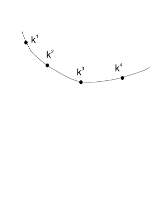
Figure 1: A kinematical state of the string: each ”particle” carries a certain fixed momentum $k$

4 Hamiltonian constraint

The physical Hilbert space is the space of solutions of both constraints diffeomorphism (19) and hamiltonian (20). To construct this space one should define the hamiltonian constraint as an operator on $H_{diff}$ and find its kernel. It is however not straightforward to define it in an explicitly diffeomorphism invariant way. Therefore given a state $|\{k\}\rangle\in H_{diff}$ the diffeomorphism invariant hamiltonian constraint operator $\tilde{\tilde{{\cal H}}}_{diff}$ will be defined as follows

$$\tilde{\tilde{{\cal H}}}_{diff}|\{k\}\rangle=\Pi\tilde{\tilde{{\cal H}}}_{aux}\pi|\{k\}\rangle$$ (35)

Here $\pi$ is a natural embedding $H_{diff}\rightarrow H_{aux}$, $\tilde{\tilde{{\cal H}}}_{aux}$ is the hamiltonian constraint operator defined on $H_{aux}$, and $\Pi$ is the projector from $H_{aux}$ to $H_{diff}$ defined in (17). The embedding $H_{diff}\rightarrow H_{aux}$ is realized by picking up for each $|\{k\}\rangle\in H_{diff}$ a representative $|\{\sigma\}\{k\}\rangle\in H_{aux}$ such that $\Pi|\{\sigma\}\{k\}\rangle=|\{k\}\rangle$, i.e. $\Pi\pi=id$. One may note that such an embedding is not unique. Moreover the resulting expression for $\tilde{\tilde{{\cal H}}}_{diff}(N)$, the hamiltonian constraint smeared with a test function $N$, will depend on the choice of $\pi$. It will be shown later that the kernel of all hamiltonian constraints, smeared with all possible test functions will nevertheless be independent of this choice.

First we shall define the action of hamiltonian constraint operator on $H_{aux}$. Note that $\tilde{\tilde{{\cal H}}}$ in (20) contains products of local operators. Therefore a point splitting regularization will be required. In our treatment the point splitting regularization will be closely related to rewriting the constraint (20) in terms of variables $U_{\sigma,k}$ (23) and $P_{\mu,\sigma_{1},\sigma_{2}}$ (26) which are well defined operators on $H_{aux}$. The variables $U_{\sigma,k}$ can be brought in the expression for hamiltonian constraint (20) due to the identity

$$k_{\mu}\partial_{\sigma}x^{\mu}=-ie^{-ik_{\mu}x^{\mu}}\partial_{\sigma}e^{ik_{\mu}x^{\mu}}=-iU_{\sigma,-k}\partial_{\sigma}U_{\sigma,k}$$ (36)

In the present paper we consider the simplest possible geometries of target space. Namely we take target space to be $d$-dimensional Minkowskian space-time and allow some of $d$ dimensions to be compactified on a torus. In this case the metric of the target space $g_{\mu\nu}$ can be made independent of coordinates, $g_{\mu\nu}=const$. One can then introduce a basis $\{k_{\mu}^{j}\}$ (not necessary orthonormal) in the target space so that the metric on it can be written as

$$g_{\mu\nu}=\sum\limits_{ij}V_{ij}k_{\mu}^{i}{k^{\prime}}^{j}_{\nu}.$$ (37)

This equation for $V_{ij}$ and $k_{\mu}^{j}$ have many different solutions. In particular one can take

$$V_{ij}=\eta_{ij}\ \ \ \ k_{\mu}^{i}={k^{\prime}}_{\mu}^{i}=e_{\mu}^{i},$$ (38)

where $\eta_{ij}$ is the Minkowskian metric and $e_{\mu}^{i}$ is an orthonormal basis. Now by using the identity (36) hamiltonian constraint (20) can be then rewritten in the form

$$\tilde{\tilde{{\cal H}}}=p_{\mu}p^{\mu}-T^{2}\sum\limits_{ij}V_{ij}U_{\sigma,-k^{i}-{k^{\prime}}^{j}}\partial_{\sigma}U_{\sigma,k^{i}}\partial_{\sigma}U_{\sigma,{k^{\prime}}^{j}}.$$ (39)

The use of the identity (36) in the definition of the hamiltonian constraint operator is similar to the construction used in loop quantum gravity in [8, 9, 10] where curvature tensor at a point is replaced by a combination of the holonomies around a set of loops originated at this point.

To promote the hamiltonian constraint in the form (39) to an operator on $H_{aux}$ one needs to regularize the operators $p_{\mu}$ and $\partial_{\sigma}U_{\sigma,k}$ entering (39) which are not well defined on the space $H_{aux}$. This can be done via smearing them with a regularized $\delta$-function

$$p_{\mu}^{\epsilon}(\sigma)=\int d\sigma^{\prime}\delta_{\epsilon}(\sigma,\sigma^{\prime})p_{\mu}(\sigma^{\prime})$$ (40)

$$\partial_{\sigma}^{\epsilon}U_{\sigma,k}=\int d\sigma^{\prime}\delta_{\epsilon}(\sigma,\sigma^{\prime})\partial_{\sigma^{\prime}}U_{{\sigma^{\prime}},k}$$ (41)

To define a regularized $\delta$-function one should introduce a background length on string space-line. A distance $L(\sigma_{1},\sigma_{2})$ between points $\sigma_{1}$ and $\sigma_{2}$ is defined as an integral of a positive defined weight 1 density $l(\sigma)$ over the interval between these points:

$$L(\sigma_{1},\sigma_{2})=\int\limits_{\sigma_{1}}^{\sigma_{2}}l(\sigma)d\sigma.$$ (42)

In the present situation it is convenient to use the step-like regularization of the $\delta$-function.

$$\delta_{\epsilon}(\sigma,\sigma^{\prime})=\left\{\begin{array}[]{ccc}\frac{l(\sigma)}{2\epsilon}&if&L(\sigma,\sigma^{\prime})<\epsilon\\ 0&if&L(\sigma,\sigma^{\prime})>\epsilon\end{array}\right.$$ (45)

The operators $p_{\mu}^{\epsilon}$ and $\partial^{\epsilon}_{\sigma}U_{\sigma,k}$ smeared with this $\delta$-function can be evaluated in terms of the operators $U_{\sigma,k}$ (23) and $P_{\mu,\sigma_{1},\sigma_{2}}$ (26):

$$p_{\mu}^{\epsilon}(\sigma)=\frac{l(\sigma)}{2\epsilon}P_{\mu,\sigma-\epsilon,\sigma+\epsilon}$$ (46)

$$\partial_{\sigma}^{\epsilon}U_{\sigma,k}=\frac{l(\sigma)}{2\epsilon}(U_{\sigma+\epsilon,k}-U_{\sigma-\epsilon,k}).$$ (47)

As a result the regularized hamiltonian constraint (39) can also be written completely in terms these operators.

$$\tilde{\tilde{{\cal H}}}^{\epsilon_{1},\epsilon_{2}}=\frac{l^{2}(\sigma)}{8\epsilon_{1}\epsilon_{2}}\Big{\{}{\cal T}(\sigma,\epsilon_{1},\epsilon_{2})+{\cal T}(\sigma,\epsilon_{2},\epsilon_{1})+{\cal V}(\sigma,\epsilon_{1},\epsilon_{2})+{\cal V}(\sigma,\epsilon_{2},\epsilon_{1})\Big{\}}$$ (48)

where

$${\cal T}(\sigma,\epsilon_{1},\epsilon_{2})=P_{\mu,\sigma-\epsilon_{1},\sigma+\epsilon_{1}}P_{\mu,\sigma-\epsilon_{2},\sigma+\epsilon_{2}}$$ (49)

is a ”kinetic” term and

$${\cal V}(\sigma,\epsilon_{1},\epsilon_{2})=T^{2}\sum\limits_{ij}V_{ij}U_{\sigma,-k^{i}-{k^{\prime}}^{j}}(U_{\sigma+\epsilon_{1},k^{i}}-U_{\sigma-\epsilon_{1},k^{i}})(U_{\sigma+\epsilon_{2},{k^{\prime}}^{j}}-U_{\sigma-\epsilon_{1},{k^{\prime}}^{j}})$$ (50)

is a ”potential” term.

Here we encounter regularization ambiguity. First, the resulting expression for potential term (50) depends on how the parameters $\epsilon_{1}$ and $\epsilon_{2}$ relate to each other. The expression with $\epsilon_{1}>\epsilon_{2}$ and expression with $\epsilon_{1}<\epsilon_{2}$ will be inequivalent even at diffeomorphism invariant level. Here the form of hamiltonian constraint is chosen to be symmetric in $\epsilon_{1}$ and $\epsilon_{2}$ (48). Second, the equation (37) for $k^{i}_{\mu}$ and $T^{2}_{ij}$ has many different solutions. This solutions result in inequivalent operators for potential term (50).

Now consider how the hamiltonian constraint (48) acts on a state $\Psi_{\{\sigma\},\{k\}}\in H_{aux}$. We will begin with considering its action at a point $\sigma_{0}$ which is not an element of a set $\{\sigma\}$ in the definition of the state $\Psi$, i.e. $\sigma_{0}\not\in\{\sigma\}$. Such point can be thought of as ”empty point”, i.e. a point with no particles at it or as a point where there is a particle with momentum equal to zero. The action of the two kinetic terms of the hamiltonian constraint, ${\cal T}(\sigma,\epsilon_{1},\epsilon_{2})$ and ${\cal T}(\sigma,\epsilon_{2},\epsilon_{1})$, yields zero. Each term in the sum in the r.h.s. of (50) results in a linear combination of four terms adding three new particles having non-zero momentum to the state, the total momentum of these three particles being zero Fig.2a.

When the hamiltonian constraint acts at a point where there is a particle having a momentum $p$ the kinetic term acts as massless Klein-Gordon operator

$${\cal T}(\sigma,\epsilon_{1},\epsilon_{2})U_{\sigma,k}=k^{\mu}k_{\mu}U_{\sigma,k}.$$ (51)

The potential term (50) results in a linear combination of terms adding two new particles with non-zero momenta located in various ways with respect to the original particle. The momentum of the original particle is changed at the same time so that the total momentum of three resulting particles be equal to the original momentum of the initial particle Fig.2b.

For neighboring points of non-zero momenta not to affect the action of the hamiltonian constraint at the point $\sigma_{0}$ $\epsilon_{1}$ and $\epsilon_{2}$ should be chosen so that for any $\sigma_{1}\in\{\sigma\}$ $L(\sigma_{0},\sigma_{1})>{\rm max}(\epsilon_{1},\epsilon_{2})$.This condition can not be satisfied for fixed $\epsilon_{1}$ and $\epsilon_{2}$ as the constraint can be applied at a point which is arbitrary close to a point with a particles having non-zero momentum. But if $\epsilon_{1}$ and $\epsilon_{2}$ very with $\sigma_{0}$ the condition $L(\sigma_{0},\sigma_{1})>{\rm max}(\epsilon_{1}(\sigma_{0}),\epsilon_{2}(\sigma_{0}))$ can be satisfied. Of course using a position dependent regularization is something unusual but this is the only possible regularization which is consistent with diffeomorphism invariance. Below we will assume that $\epsilon_{1}$ and $\epsilon_{2}$ are such functions of $(\sigma_{0})$ that the above condition is satisfied and that $\epsilon_{1}>\epsilon_{2}$.

Note that after applying the hamiltonian constraint at $H_{aux}$ we will then project the resulting state on $H_{diff}$. This makes the precise positions of the tree particles added irrelevant to the final result. Only relative order of these three points matters. Therefore the diffeomorphism invariant result of the action of hamiltonian constraint can be schematically shown as ”moves” ”no particles into three particles” ($0\rightarrow 3$) (the action at an empty point) or ”one particle into three particles” ($0\rightarrow 3$) (the action at a point with a particle having non-zero momentum) (see Fig.2).

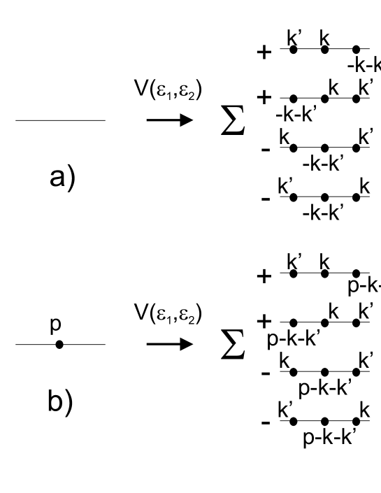
Figure 2: The action of the potential term ${\cal V}(\epsilon_{1},\epsilon_{2})$ of the hamiltonian constraint on a kinematical state: a) The action at an empty point b) The action at a point with a particle having a momentum $p$

One of the key properties of loop quantum gravity which makes it an easily treatable theory is that the action of hamiltonian constraint on basis states is purely combinatorial. It has non-vanishing action only on the points where Wilson loops has intersections while non-intersecting loops are exactly annihilated by it [11]. It is desirable here that the regularized hamiltonian constraint of the string have the same property, i.e. annihilate the state while acting at a point with no particles. There is a possibility of achieving this. One can note that the momenta at the three new points are arbitrary, any choice of them will reproduce the original classical expression after removing the regulator. One therefore can make use of this arbitrariness and impose an additional constraint on momenta at the three new points. The following three possible types of such constraints result in annihilating of the empty points by the hamiltonian constraint:

$$k+k^{\prime}=0,$$ (52)

$$k^{\prime}=-2k,$$ (53)

$$k=-2k^{\prime}.$$ (54)

This can be seen by imposing any of these constraints on linear combination of the terms depicted at Fig.2a. Then by diffeomorphism transformation the first and the second terms in this linear combination can be turned into the third and the fourth and they all cancel each other. The cancellation will not happen at a point where there is a particle with non-zero momentum Fig.2b. Therefore there is only a finite number of points at string space-line at which the action of the hamiltonian constraint is non-zero.

For further constructions we will need the matrix element of the hamiltonian constraint (48) smeared with a test function ${\cal N}$

$${\cal H}[{\cal N}]=\int d\sigma{\cal N}(\sigma)\tilde{\tilde{{\cal H}}}(\sigma)$$ (55)

between two diffeomorphism invariant states $|\{k\}\rangle$ and $|\{k^{\prime}\}\rangle$. Note that the operator ${\cal H}[{\cal N}]$ in (55) is a non-diffeomorphism invariant operator defined on $H_{aux}$. However given its action on non-diffeomorphism invariant states on can define its action on $H_{diff}$ via (35).

Now one should define the smearing of the operator (48) with a test function. A consistent definition takes the following steps:

1. Take the regularized expression (48) for $\tilde{\tilde{{\cal H}}}^{\epsilon_{1},\epsilon_{2}}$ acting on $H_{aux}$ and project the result on $H_{diff}$. As it has been mentioned above only the action at the points with a particles having non-zero momentum will survive. Also in projecting the result on $H_{diff}$ any dependence on regularization parameters $\epsilon_{1}$ and $\epsilon_{2}$ will disappear.

2. Embed the obtained result into $H_{aux}$. This is necessary because the expression (55) contains a hamiltonian constraint defined on $H_{aux}$. On the other hand we can not simply substitute the hamiltonian constraint (48) in its original form into the equation (55) as in this case it would contain the action on each point of the string space-line continuum which is difficult to control. By projecting the result on $H_{diff}$ and then embedding it back into $H_{aux}$ the action of $\tilde{\tilde{{\cal H}}}^{\epsilon_{1},\epsilon_{2}}$ is reduced to that on finite number of points. The embedding of $H_{diff}$ into $H_{aux}$ is ambiguous, the positions of the points at the string space-line can be chosen arbitrary. To restore the information about the regularization one should place the points added by the action of the hamiltonian constraint at the distances $\epsilon_{1}$ and $\epsilon_{2}$ from the original point at which the new points where added. To account the fact that the points with particles having non-zero momenta are the only points where the constraint have a non-zero action one should multiply the new expression for $\tilde{\tilde{{\cal H}}}^{\epsilon_{1},\epsilon_{2}}(\sigma)$ by a characteristic function of $\epsilon_{1}$-vicinity of those points.

$$\tilde{\tilde{{\cal H}}}^{\epsilon_{1},\epsilon_{2}}(\sigma)|\{\sigma\},\{k\}\rangle=$$

$$\sum\limits_{\alpha}\chi_{[\sigma_{\alpha}-\epsilon_{1},\sigma_{\alpha}+\epsilon_{1}]}(\sigma)\frac{l^{2}(\sigma)}{8\epsilon_{1}\epsilon_{2}}\Big{\{}{\cal T}(\sigma,\epsilon_{1},\epsilon_{2})+{\cal T}(\sigma,\epsilon_{2},\epsilon_{1})+{\cal V}(\sigma,\epsilon_{1},\epsilon_{2})+{\cal V}(\sigma,\epsilon_{2},\epsilon_{1})\Big{\}}|\{\sigma\},\{k\}\rangle,$$ (56)

where

$$\chi_{[\sigma_{\alpha}-\epsilon_{1},\sigma_{\alpha}+\epsilon_{1}]}(\sigma)=\left\{\begin{array}[]{ccc}1&if&L(\sigma,\sigma_{\alpha})<\epsilon_{1}\\ 0&if&L(\sigma,\sigma_{\alpha})>\epsilon_{1}\end{array}\right.$$ (59)

The multiplication by of the expression for the hamiltonian constraint by $\sum\limits_{\alpha}\chi_{[\sigma_{\alpha}-\epsilon_{1},\sigma_{\alpha}+\epsilon_{1}]}(\sigma)$ is the summary result of its projection on $H_{diff}$ and then embedding into $H_{aux}$.

3. Smear the hamiltonian constraint obtained in the previous step with a test function ${\cal N}$. Because the hamiltonian constraint is a density of the weight 2 with respect to diffeomorphisms of the space line of the string the test function ${\cal N}$ in (55) has to be a density of the weight -1. We will need also scalar test function $N$ related to ${\cal N}$ by

$$N=\frac{l(\sigma)}{2\epsilon_{2}}{\cal N}$$ (60)

The relation between $N$ and ${\cal N}$ depends on a background metric $l$, but because the test function is arbitrary this doesn’t introduce any ambiguity. By taking into account that

$$\chi_{[\sigma_{\alpha}-\epsilon_{1},\sigma_{\alpha}+\epsilon_{1}]}(\sigma)\frac{l(\sigma)}{2\epsilon_{1}}=\delta_{\epsilon_{1}}(\sigma,\sigma_{\alpha})$$ (61)

the resulting expression can be written in the form:

$${\cal H}[{\cal N}]|\{\sigma\},\{k\}\rangle=$$

$$\int d\sigma N(\sigma)\sum\limits_{\alpha}\delta_{\epsilon_{1}}(\sigma,\sigma_{\alpha})\frac{1}{2}\Big{\{}{\cal T}(\sigma,\epsilon_{1},\epsilon_{2})+{\cal T}(\sigma,\epsilon_{2},\epsilon_{1})+{\cal V}(\sigma,\epsilon_{1},\epsilon_{2})+{\cal V}(\sigma,\epsilon_{2},\epsilon_{1})\Big{\}}|\{\sigma\},\{k\}\rangle.$$ (62)

4. Finally we can remove the regulator in the equation (62) and perform the integration over $\sigma$. The result will be

$${\cal H}[{\cal N}]|\{\sigma\},\{k\}\rangle=\sum\limits_{\{\sigma\}}N(\sigma_{\alpha}){\cal H}(\sigma_{\alpha})|\{\sigma\},\{k\}\rangle,$$ (63)

where

$${\cal H}(\sigma_{\alpha})=\lim_{\epsilon_{1},\epsilon_{2}\rightarrow 0}\Big{\{}{\cal T}(\sigma,\epsilon_{1},\epsilon_{2})+{\cal T}(\sigma,\epsilon_{2},\epsilon_{1})+{\cal V}(\sigma,\epsilon_{1},\epsilon_{2})+{\cal V}(\sigma,\epsilon_{2},\epsilon_{1})\Big{\}}$$ (64)

By definition of scalar product on diffeomorphism invariant states (17) one can write the matrix element of $H[{\cal N}]$ as follows

$$\langle\{k^{\prime}\}|H[{\cal N}]|\{k\}\rangle=\sum\limits_{\{\sigma\}}N(\sigma_{\alpha})\langle\{k^{\prime}\}|H(\sigma_{\alpha})|\{\sigma\},\{k\}\rangle$$ (65)

One can see that the resulting expression for matrix element is not diffeomorphism invariant. It depends on the locations of the points $\sigma_{\alpha}$ which represent the embedding $\pi$ of a state $|\{k\}\rangle\in H_{diff}$ to a state $|\{\sigma\},\{k\}\rangle\in H_{aux}$. However to obtain a physical matrix element a functional integration over $N(\sigma)$ should be performed and as it was shown in [14] the dependence on the embedding $\pi$ can be removed from the resulting expression.

A matrix element entering the sum in the r.h.s. of (65) can be evaluated explicitly by using the expression (48) for the regularized hamiltonian constraint

$$\langle\{k^{\prime}\}|H(\sigma_{\alpha})|\{\sigma\},\{k\}\rangle = k_{\alpha,\mu}k_{\alpha}^{\mu}\langle\{k^{\prime}\}|\{k\}\rangle-T^{2}\sum\limits_{ij}V_{ij}\langle\{k^{\prime}\}|K_{\alpha,ij}\{k\}\rangle$$ (66)

$$= k_{\alpha,\mu}k_{\alpha}^{\mu}\delta_{\{k^{\prime}\}\{k\}}-T^{2}\sum\limits_{ij}V_{ij}\delta_{\{k^{\prime}\}K_{\alpha,ij}\{k\}}$$

Here the operator $K_{\alpha,ij}$ is defined as follows (recall that the diffeomorphism invariant state $|\{k\}\rangle$ is defined as an ordered set of momenta $(k_{1},...,k_{N})$):

$$K_{\alpha,ij}(k_{1},...,k_{\alpha},...,k_{N})=(k_{1},...,k_{i},k^{\prime}_{j},k_{\alpha},...,k_{N})+(k_{1},...,k_{\alpha},k^{\prime}_{j},k_{i},...,k_{N})$$

$$-(k_{1},...,k^{\prime}_{i},k_{\alpha},k_{j},...,k_{N})-(k_{1},...,k^{\prime}_{j},k_{\alpha},k_{i}...,k_{N})+(k_{i}\leftrightarrow k^{\prime}_{j})$$ (67)

In order to allow the this hamiltonian constraint to convey momentum from one point in original state to another one should take the hamiltonian constraint in (75) to be symmetric one ${\cal H}[N]={\cal H}_{sym}[N]$, i.e. to allow it not only create but also annihilate new points in a state,

$$\langle\{k^{\prime}\}|{\cal H}_{sym}[N]|\{k\}\rangle=\langle\{k^{\prime}\}|{\cal H}[N]|\{k\}\rangle+\overline{\langle\{k\}|{\cal H}[N]|\{k^{\prime}\}\rangle}$$ (68)

Now given the expression for the hamiltonian constraint it’s straightforward to calculate the quantum constraint algebra. It turns out to be very similar to that in loop quantum gravity [12],[13]:

$$\big{[}{\cal D},{\cal D}\big{]}\sim{\cal D},$$

$$\big{[}{\cal H},{\cal D}\big{]}\sim{\cal H},$$

$$\big{[}{\cal H},{\cal H}\big{]}=0$$ (69)

Because of the last equation this algebra is not isomorphic to the classical constraint algebra. This is the first problem we encounter.

Now one can try to solve the constraint equation defined. First of all one can note that the vacuum (the state with no particles) is a solution of both constraints. The first non-trivial solution is a state with a single particle located at a closed string:

$$|\{k\}\rangle=e^{ik_{1,\mu}X^{\mu}(\sigma_{1})}.$$ (70)

It is easy to see that the four terms resulting from the potential term of the hamiltonian constraint and depicted at Fig.2b cancel each other if we connect the free ends of the string together thereby forming a closed string. The kinetic term in the hamiltonian constraint disappears provided that the momentum $k_{1,\mu}$ entering (70) is null, $k_{1,\mu}k_{1}^{\mu}=0$. This state should be identified with the well known tachionic mode of the string. This is because the particle is a scalar and also in string theory the tachionic state is produced by the insertion of vertex operator of the form (70) into string world-sheet. Generally due to the anomaly in string theory the states of the string should be taken to be solutions of a shifted hamiltonian constraint ${\cal H}^{\prime}={\cal H}+constant$. The constant would play the role of the squared mass of the mode and being negative would make the mode tachionic. However the present regularization of the hamiltonian constraint produces an anomaly-free constraint algebra and therefore the scalar string mode have to be massless. Another problem is that the solution (70) exists only for the closed string, this can not be generalized to the case of the open string.

The following non-trivial solutions to all the constraints are expected to be higher modes of the string. Because we don’t have the higher modes vertex operators at our disposal they are to be constructed from tachionic vertex operators. The solution to all the constraints can be sought in a form of an infinite linear combination of terms with various numbers of tachionic vertex operators inserted. This can be derived via an expansion of the projector on the physical states. This is what the next section is devoted to.

5 The projector on the physical states

The construction of projector on the physical Hilbert space of the string and its interpretation will closely followed to those introduced in [14]. It is based on perturbative expansion of the functional integral

$$P\sim\prod\limits_{\sigma}\delta({\cal H}(\sigma))\sim\int[DN]e^{-i\int d\sigma N(\sigma){\cal H}(\sigma)}$$ (71)

Given the matrix element of this operator between general two general states from $H_{diff}$

$$\langle\{k^{\prime}\}|P|\{k\}\rangle=\int[DN]\langle\{k^{\prime}\}|e^{-iH[N]}|\{k\}\rangle$$ (72)

we can define the physical Hilbert space $H_{phys}$ over the pre-Hilbert space $H_{diff}$ by the quadratic form

$$\langle\{k^{\prime}\}||\{k\}\rangle_{phys}=\langle\{k^{\prime}\}|P|\{k\}\rangle.$$ (73)

In [14] the functional integral is regularized by

$$|N(\sigma)|<N_{max},$$ (74)

where $N_{max}$ is a certain constant. The physical limit is recovered for $N_{max}\rightarrow\infty$. Then the exponent in (72) is replaced by6 its Taylor series. The resulting expression is therefore involve matrix elements of different powers of ${\cal H}[N]$ which as we have seen in the previous section depend on the values of $N$ at a certain set of points and therefore are not diffeomorphism invariant. However the expression (72) as well as the regularization (74) are diffeomorphism invariant. Therefore we can insert an integration over the diffeomorphism group in the expression (72). The resulting expression then reads

$$\langle\{k^{\prime}\}|P_{N_{max}}|\{k\}\rangle=\int_{Diff}D\phi\int_{|N(\sigma)|<N_{max}}DN\langle{\cal U}(\phi)\{k^{\prime}\}\{\sigma^{\prime}\}|\left(\sum\limits_{n=0}^{\infty}\frac{(-i)^{n}}{n!}({\cal H}[N])^{n}\right)|\{k\}\rangle.$$ (75)

It can be interpreted as a sum over planar Feynmann diagrams with vertices depicted on Fig.3.

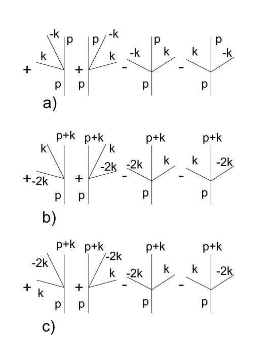
Figure 3: Sets of diagrams appearing as a result of the action of the hamiltonian constraint at a point with a particle having a momentum $p$ ; a) with constraint (52), b) with constraint (53)

, c) with constraint (54)

Given the hamiltonian constraint found in the previous section, the spin-foam diagrams of this model become very similar to those of two-dimensional $\phi^{4}$-model. They are comprised by four-valent vertices and lines connected them. There is however a certain difference between them. First, no integration over the momenta in closed loops is required. The momentum flowing around a closed loop is a free parameter which appears in regularization. $\phi^{4}$-model can however be recovered by taking a sum over all the possible regularization parameters. Another feature of $\phi^{4}$ which is lacking in the present model is the possibility of $2\rightarrow 2$ move. The later probably reflects the general difficulty with application of canonical quantization to a generally covariant theory. Space-time covariance get lost in canonical approach and to recover it a resulting theory should be modified e.g. by adding some extra moves [15], [16]. Finally, an additional constraint (52) or (53) or (54) on momenta meeting at a vertices needs to be imposed. To recover $\phi^{4}$-model one should make the resulting theory free of this constraints. One can easily see that the constraints (53) and (54) are not invariant with respect to renormalization of the tension which in the present case plays the role of coupling constant. By applying block transformation to four valent vertices subject to these constraint one can recover the general vertex of $\phi^{4}$-model with the only constraint being the conservation of momentum. The vertices with constraint (52) remain unchanged under renormalization, but this is not an interesting case because such vertices do not convey momenta from one point to another. Therefore, one can conclude that in any case we should end up with the two-dimensional $\phi^{4}$-model. The only freedom remained is the domain of integration over the momenta flowing around closed loops.

6 Hamiltonian constraint, second version

The suggested version of the hamiltonian constraint leave us with a theory which is considerably different from ordinary string theory. There are several indications that string theory in its usual form can probably not be recovered from the model obtained. Firstly, in conformal field theory the expectation value of a product of three vertex operators is not equal to zero. On the other hand the model we obtained is similar to $\phi^{4}$-model which does not contain a transition involving three vertex operators. Nor can three valent vertices be recovered via block transformation. Besides, the model for representing a discretized string is generally taken to be $\phi^{3}$ [17]. Another difference between them is that as it was mentioned in section 4 the first version of hamiltonian constraint is anomaly-free and the same is true of the diffeomorphism constraint. Alternatively, in ordinary string theory quantum constraint algebra contains an anomaly which is absent only in critical dimension of target space $d=26$.

There is however another regularization of the hamiltonian constraint which results in a model having much more similarity with ordinary quantization of the string. By making use of regularization ambiguity one can get a theory which resemble $\phi^{3}$-model and contains an anomaly which can be cancelled by tuning the parameters of the theory. Given most general regularization of ${\cal H}$ (48) one can first set $\epsilon_{1}=\epsilon_{2}=\epsilon$, momenta at coinciding points being added to each other. Then one can require that the action of the hamiltonian constraint cancel the momenta at the points where it acts , i.e. $p(\sigma)-k-k^{\prime}=0$. This is another piece of position dependence in the regularization (recall that $\epsilon$ is also position dependent). The resulting hamiltonian constraint can be written as follows,

$$\tilde{\tilde{{\cal H}_{2}}}^{\epsilon}=\frac{l^{2}(\sigma)}{4\epsilon^{2}}\Big{\{}{\cal T}_{2}(\sigma,\epsilon)+{\cal V}_{2}(\sigma,\epsilon)\Big{\}}$$ (76)

where

$${\cal T}_{2}(\sigma,\epsilon)=P_{\mu,\sigma-\epsilon,\sigma+\epsilon}P_{\mu,\sigma-\epsilon,\sigma+\epsilon}$$ (77)

and

$${\cal V}_{2}(\sigma,\epsilon)|\{\sigma\},\{p\}\rangle$$ (78)

$$= T^{2}\sum\limits_{ij}V_{ij}U_{\sigma,-p}(U_{\sigma+\epsilon,p/2-k^{i}}-U_{\sigma-\epsilon,p/2-k^{i}})(U_{\sigma+\epsilon,p/2+k^{i}}-U_{\sigma-\epsilon,p/2+k^{i}})|\{\sigma\},\{p\}\rangle$$

$$= T^{2}\sum\limits_{ij}V_{ij}[2U_{\sigma,-p}U_{\sigma+\epsilon,p}-U_{\sigma+\epsilon,p/2+k^{i}}U_{\sigma-\epsilon,p/2-k^{i}}-U_{\sigma+\epsilon,p/2-k^{i}}U_{\sigma-\epsilon,p/2+k^{i}}]|\{\sigma\},\{p\}\rangle$$

$$- T^{2}\sum\limits_{ij}V_{ij}[U_{\sigma,-p}U_{\sigma+\epsilon,p}-U_{\sigma,-p}U_{\sigma-\epsilon,p}]|\{\sigma\},\{p\}\rangle.$$

In the above equation by $p$ we meant $p(\sigma)$ – the momentum at the point of the string where the operator acts. It is easy to see that as $\epsilon\rightarrow 0$ $U_{\sigma,-p}U_{\sigma+\epsilon,p}$ is the identity operator and $[U_{\sigma,-p}U_{\sigma+\epsilon,p}-U_{\sigma,-p}U_{\sigma-\epsilon,p}]/\epsilon$ is a diffeomorphism. The identity operator will introduce a constant term into the hamiltonian constraint, which is similar to the appearance of a central term in the Virasoro algebra in string theory in the Fock representation from commutator between the creation and annihilation operators. Thus, this version of the hamiltonian constraint contains moves $0\rightarrow 0$, $0\rightarrow 2$, $1\rightarrow 1$, and $1\rightarrow 2$, Fig.4.

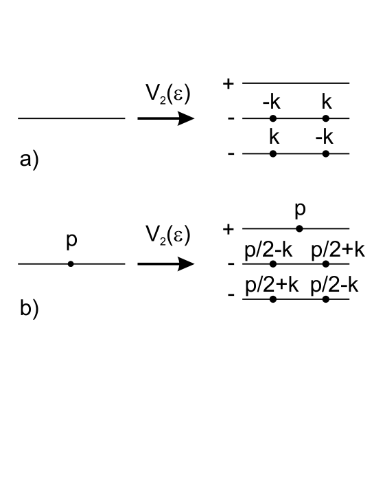
Figure 4: Action of the potential term of the hamiltonian constraint defined in (78) on a kinematical state. a) at an empty point. b) at a point with a particle having a nonzero momentum

Moves $0\rightarrow 0$ and $1\rightarrow 1$ correspond to an additive constant $c=\sum\limits_{i,j=1}^{d}T_{ij}$ in the hamiltonian constraint. This term results in an anomaly in the constraint algebra as the commutator between the hamiltonian and the diffeomorphism constraints should close on the hamiltonian constraint but the additive constant commutes with constraint and therefore the hamiltonian constraint will not be reproduced. It is natural to suggest that this is analogous to the well known conformal anomaly in string theory, $c$ playing the role of the central charge. In string theory conformal anomaly can be cancelled by tuning the dimension of space, $d=26$. In our treatment $c$ can be thought of as a vacuum energy of the string and (when the hamiltonian constraint acts at a point with no particles) or when the hamiltonian constraint acts at a point where there is a particle it can be interpreted as a squared mass of this particle (in this case the massless Klein-Gordon operator $k^{\mu}k_{\mu}$ acting on this particle is replaced by $k^{\mu}k_{\mu}+c$).

A natural question then arises: is there a possibility to cancel this anomaly by tuning parameters of the theory? If so, will it constraint the dimension of space to be equal to 26? The answer on this question would require a more detailed consideration. For the present, one can give an argument that the central charge can be changed by changing the parameters of the theory. As in ordinary interacting quantum field theory, the transition amplitude between two states can be represented as a sum over Feynmann diagrams. The contributions from some of these diagrams can be taken into account by a redefinition of the constants of the theory. The same can be done here. First, the moves $0\rightarrow 2$ give rise to vacuum loops in Feynmann diagrams. All these diagrams contribute to the vacuum energy of the theory which was initially equal to $c$.

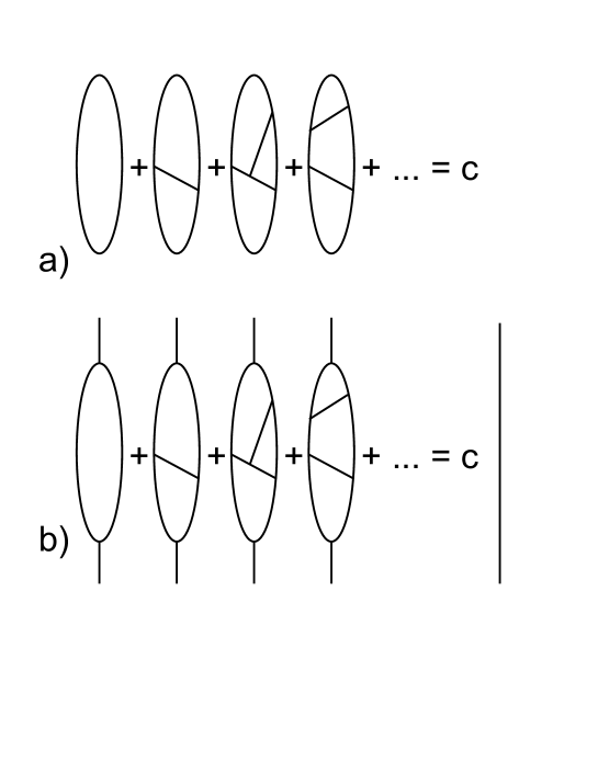
Figure 5: a) corrections to the vacuum energy of the string; b) corrections to the mass of the particles

Therefore if the sum over all vacuum loops is equal to $c$ as it is shown on Fig.5a, the vacuum energy of the string is equal to zero. Similarly, diagrams shown on Fig.5b contribute to the mass of the particle and can cancel it under certain conditions. It is important to note that the condition of setting the vacuum energy to zero is consistent with the condition of setting the masses of the particles to zero. This is due to the apparent one to one correspondence between the set of diagrams shown on Fig.5a and that shown on Fig.5b. This consistency allow one in principle to cancel the anomaly by setting the vacuum energy and masses of the particles to zero.

7 Discussion

The main issue the proposed model is intended to address is the problem of continuum limit in loop quantum gravity. Ordinary string theory based on Fock space quantization have the right continuum limit. Therefore in the present context this problem reduces to that of finding a relation between the resulting model we obtained and the ordinary quantum string.

There is another indication that the right way of looking for continuum limit of this model is through the relation between it and ordinary string theory. Let us recall that the problem of continuum limit in loop quantum gravity consists of two parts. First part is the problem of the existence of moves which would convey interaction between neighboring vertices of spin network. This problem has no analog in the present model: both versions of the hamiltonian constraint proposed allow a creation of a particle by one particle in an initial state and its subsequent absorbtion by a neighboring particle. If the first part of the problem is solved there appears another one: in continuum limit perturbations of a state of the theory should propagate arbitrary far, while in a general discrete model with interaction between nearest neighbors perturbations decay at a certain distance. The later can be interpreted as that the particles which are responsible for mediating the interaction acquire a mass. This problem is generally solved by tuning parameters of a model so that the mass of these particles is set to zero. It is interesting to note in this connection that by requiring that the resulting theory be anomaly-free we set the masses of the particles associated with vertex operators to zero. However it is still unclear whether these particles can be identified with those responsible for mediating perturbations of a state of the string.

The easiest way to establish the equivalence between this model and ordinary string theory would be to show that the partition function of three vertex operators, which is a well known quantity in string theory, coincides with the amplitude of the move $1\rightarrow 2$ given by the hamiltonian constraint with renormalized parameters. This is not straightforward to do because to find the renormalized values of parameters one should perform a summation over all the diagrams in the series. Therefore, it will be necessary to find a natural small parameter in which the expansion is made.

In QFT models such as $\phi^{3}$ the only such parameter is the coupling constant. In our treatment the role of coupling constant is played by string tension. The model in the limit $T\rightarrow 0$ corresponds to kinematical picture, the only difference being that the particles should now obey Klein-Gordon equation $k_{\mu}k^{\mu}=0$. The hamiltonian constraint of the model can therefore be divided into two parts: a free hamiltonian and an interaction term. One can then construct ”interaction representation” for this model by associating an exact solution of the free hamiltonian to each line in the diagrams and an interaction term to each vertex. In this case Feynmann diagrams can be understood as an expansion in powers of string tension. Therefore this model should work well in the limit of small tension.

It is interesting to consider the role played by T-duality in this model. The critical radius of compactification below which string modes become redundant is proportional to the inverse tension of the string. The kinematics of this model corresponds to zero tension and therefore the critical radius of compactification is equal to infinity. This means that we are always below the critical radius and there is a certain redundancy in the description of kinematical state. This redundancy manifest itself in the fact that e.g. a state with two particles having momenta $k^{1}$ and $k^{2}$ is kinematically equivalent with a state with one particle having a momentum $k^{1}+k^{2}$. Therefore all the kinematical states of the string can be made of ”elementary” particles having the smallest possible momentum. This picture has a close similarity with string bit models [6, 7]. How to extend this picture on dynamics is still unclear.

String bit models describe string theory in light cone frame $x^{-}=x^{0}-x^{d}=0$. In this connection it is interesting to note that in light cone frame the considerations of this paper would undergo a considerable simplification. Recall that there was a problem with making the hamiltonian constraint “combinatorial”, i.e. acting only on a finite set of points. In light cone frame this is satisfied automatically and therefore neither an additional constraint on the regularization parameters (like in section 4) nor renormalization of the vacuum energy (like in section 6) is required. This is because in this frame the longitudinal momentum is always positive $p_{-}\geq 0$. This property together with conservation of momenta $\sum p_{-}^{i}=0$ results in setting all the longitudinal momenta created by an action of hamiltonian constraint to zero $p_{-}^{i}-=0$. In quantum field theory in light cone frame the point $p_{-}=0$ is called “zero mode”. It is a singular point of the theory and a regularization is required here. One generally introduces a regularization condition $p_{-}>\epsilon>0$ and therefore zero mode can be neglected. In the present case there is a singularity in the hamiltonian constraint for small added momentum $k$. It can be seen from the equation (37) that as $k_{\mu}^{i}\rightarrow 0$, $T^{2}_{ij}\rightarrow\infty$. Therefore the infrared cutoff will be necessary in this theory anyway and this in particular should rule the zero mode out.

References

- [1] C. Rovelli, Loop Quantum Gravity. Living Reviews in Relativity, 1998-1, http://www.livingreviews.org/ and e-print: gr-qc/9710008.
- [2] C. Rovelli and L. Smolin, Knot theory and quantum gravity. Phys. Rev. Lett. 61 (1988) 1155.
- [3] C. Rovelli and L. Smolin, Loop representation of quantum general relativity. Nucl. Phys. B331 (1990) 80.
- [4] M. Varadarajan, Fock representations from U(1) holonomy algebras, Phys. Rev D61, 104001 (2000). M. Varadarajan, Photons from quantized electric flux representations, gr-qc/0104051
- [5] A. Ashtekar, J. Lewandowski, Relation between polymer and Fock excitations, gr-qc/0107043
- [6] I. Klebanov and L. Susskind Nucl. Phys. B309 (88) 175
- [7] C. Thorn Published in Sakharov Conf on Physics, Moscow, (91):447-454
- [8] C. Rovelli and L. Smolin, Physical hamiltonian in non-perturbative quantum gravity, Phys. Rev. Lelt. 72, 446 (1994)
- [9] T. Thiemann, Anomaly-free formulation of non-perturbative, four-dimensional Lorentzian quantum gravity. Phys. Lett. B380 (1996) 257, e-print: gr-qc/9606088.
- [10] T. Thiemann, Quantum Spin Dynamics (QSD) Class. Quant. Grav. 15 (1998) 839, e-print: gr-qc/9606089.
- [11] T. Jacobson and L. Smolin, Nonperturbative quantum geometries. Nucl. Phys. B299 (1988) 295.
- [12] Lewandowski, J., and Marolf, D., “Loop constraints: A habitat and their algebra”, (1997), [Online Los Alamos Preprint Archive]: cited on September 1997, http://xxx.lanl.gov/abs/gr-qc/?
- [13] Gambini, R., Lewandowski, J., Marolf, D., and Pullin, J., “On the consistency os the constraint algebra in spin network quantum gravity”, (September, 1997), [Online Los Alamos Preprint Archive]: cited on September 1997, http://xxx.lanl.gov/abs/?
- [14] C. Rovelli, The projector on physical states in loop quantum gravity, gr-qc/9806121
- [15] F. Markopoulou and L. Smolin Causal evolution of spin networks, Nucl.Phys. B508 (1997) 409-430 gr-qc/9702025
- [16] Reisenberger, M., and Rovelli, C., “Sum over Surfaces form of Loop Quantum Gravity”, Phys. Rev., D56, 3490–3508, (1997). For a related online version see: M. Reisenberger, et al., “Sum over Surfaces form of Loop Quantum Gravity”, (December, 1996), [Online Los Alamos Preprint Archive]: cited on September 1997, http://xxx.lanl.gov/abs/gr-qc/9612035.
- [17] J. Ambjorn, D. Boulatov, V.A. Kazakov THE BOSONIC STRING SIMULATED AS PHI**3 GRAPHS, Nucl.Phys.Proc.Suppl.17:617-620,1990 J. Ambjorn, D. Boulatov, V.A. Kazakov THE BOSONIC STRING REPRESENTED AS PHI**3 GRAPHS: NEW MONTE CARLO SIMULATIONS Mod.Phys.Lett.A5:771,1990