1.0

1.0 This thesis describes the application of numerical techniques to solve Einstein’s field equations in three distinct cases.
First we present the first long-term stable second order convergent Cauchy characteristic matching code in cylindrical symmetry including both gravitational degrees of freedom. Compared with previous work we achieve a substantial simplification of the evolution equations as well as the relations at the interface by applying the method of Geroch decomposition to both the inner and the outer region. We use analytic vacuum solutions with one and two gravitational degrees of freedom to demonstrate the accuracy and convergence properties of the code.

In the second part we numerically solve the equations for static and dynamic cosmic strings of infinite length coupled to gravity and provide the first fully non-linear evolutions of cosmic strings in curved spacetimes. The inclusion of null infinity as part of the numerical grid allows us to apply suitable boundary conditions on the metric and the matter fields to suppress unphysical divergent solutions. The resulting code is checked for internal consistency by a convergence analysis and also by verifying that static cosmic string initial data remain constant when evolved. The dynamic code is also shown to reproduce analytic vacuum solutions with high accuracy. We then study the interaction between a Weber-Wheeler pulse of gravitational radiation with an initially static string. The interaction causes the string to oscillate with frequencies proportional to the masses of its scalar and vector field. After the pulse has largely radiated away, the string continues to ring but the oscillations slowly decay and eventually the variables return to their equilibrium values.

In the final part of the thesis we probe a new numerical approach for highly accurate evolutions of neutron star oscillations in the case of radial oscillations of spherically symmetric stars. For this purpose we decompose the problem into a static background governed by the Tolman-Oppenheimer-Volkoff equations and time dependent perturbations. In contrast to conventional treatments, the fully non-linear form of the resulting perturbative equations is used. In an Eulerian formulation of the problem the movement of the surface of the star relative to the fixed numerical grid leads to difficulties in the numerical as well as the algebraic analysis. In order to alleviate the surface problem we use a simplified neutron star model to study the non-linear coupling of eigenmodes. By virtue of the high accuracy of our numerical method we are able to analyse the excitation of eigenmodes over a wide range of initial amplitudes. We find two distinct regimes, a weakly non-linear regime where the coefficients of higher order eigenmodes increase quadratically with the initial amplitude and a moderately non-linear regime where this increase steepens and an initially present mode of order $j$ couples more efficiently to modes of order $2j$, $3j$ and so on.

We conclude this work with the development of a fully non-linear perturbative Lagrangian code. We demonstrate how the difficulties at the surface of the star that arise in an Eulerian framework are naturally resolved in the Lagrangian formulation. This code is used to study the formation of discontinuities near the surface for initial data of low amplitude.

1.0

Acknowledgements

In the vain hope of achieving completeness I would like to express my gratitude to the following people.
My supervisor Ray d’Inverno for making this whole project possible and for all support and suggestions I have received in the course of the last three years.
Nils Andersson, Carsten Gundlach and James Vickers for many suggestions, discussions, encouragement and constructive criticism of my work.
All other members of the Southampton relativity group who provided a phantastic working environment and were barely ever short of encouraging comments, support and ideas.
My colleague Robert Sjödin with whom I worked jointly on the cosmic string project. The derivation of the equations for a cosmic string in section 4 has been done in collaboration with him and he reformulated the analytic vacuum solutions used in section 3 and 4 in the way they are implemented in the codes.
Last but not least Philippos Papadopoulos of the University of Portsmouth for his many suggestions, ideas and support concerning the work in section 5.

Notation

Unless stated otherwise, the following conventions apply. Greek indices run from 0 to 3, whereas Latin indices are used for 3-dimensional quantities. We will generally represent vectors and tensors of higher rank with boldfaced letters (e.g. T). Sometimes we will denote vectors, i.e. tensors of rank (1,0), by partial differential operators (e.g. $\mathchoice{{\hbox{\boldmath$\displaystyle\partial$}}}{{\hbox{\boldmath$\textstyle\partial$}}}{{\hbox{\boldmath$\scriptstyle\partial$}}}{{\hbox{\boldmath$\scriptscriptstyle\partial$}}}_{t}$). If we need to distinguish between a one-form and a vector, the one-form will be marked with a tilde (e.g. $\tilde{\hbox{\vec{u}}}$). If a one-form is the exterior derivative of a scalar function $f$, it will be denoted by $\hbox{\vec d}f$ and the tilde will be omitted. If v is a vector, then $\tilde{\hbox{\vec v}}$ is the associated one-form, i.e. $\tilde{\hbox{\vec v}}=\hbox{\vec g}({\hbox{\vec v}},.)$. In coordinate free language the contraction of a one-form $\tilde{\hbox{\vec{u}}}$ with a vector v will be written as $\langle\tilde{\hbox{\vec u}},{\hbox{\vec v}}\rangle$. The 4-dimensional Riemann tensor and its contractions will be denoted by the standard R. For the 3-dimensional Riemann tensor we always use $\mathcal{R}$. We will use square brackets to denote the commutator as is done in quantum mechanics, so for example $[\nabla_{\alpha},\nabla_{\beta}]=\nabla_{\alpha}\nabla_{\beta}-\nabla_{\beta}\nabla_{\alpha}$. Throughout this work we will use natural units with $c=1=G$ and the sign convention “$-++\,+$” for the metric.

1 Introduction

In 1915 Albert Einstein published a geometrical theory of gravitation: The General Theory of Relativity. He presented a fundamentally new description of gravity in the sense that the relative acceleration of particles is not viewed as a consequence of gravitational forces but results from the curvature of the spacetime in which the particles are moving. As long as no non-gravitational forces act on a particle, it is always moving on a “straight line”. If we consider curved manifolds there is still a concept of straight lines which are called geodesics, but these will not necessarily have the properties we intuitively associate with straight lines from our experience in flat Euclidean geometry. It is, for example, a well known fact that two distinct straight lines in 2-dimensional flat geometry will intersect each other exactly once unless they are parallel in which case they do not intersect each other at all. These ideas result from the fifth Euclidean postulate of geometry which plays a special role in the formulation of geometry. It is a well known fact that one needs to impose it separately from the first four Euclidean postulates in order to obtain flat Euclidean geometry. It was not realised until the work of Gauss, Lobachevsky, Bolyai and Riemann in the 19th century that the omission of the fifth postulate leads to an entirely new class of non-Euclidean geometries in curved manifolds. A fundamental feature of non-Euclidean geometry is that straight lines in curved manifolds can intersect each other more than once and correspondingly diverge from and converge towards each other several times. In order to illustrate how these properties give rise to effects we commonly associate with forces such as gravitation, we consider two observers on the earth’s surface, say one in Southampton and one in Hamburg. We assume that these two observers start moving due south in “straight lines” as for example guided by an idealised compass exactly pointing towards the south pole. If we follow their separate paths we will discover exactly the ideas outlined above. As long as both observers are in the northern hemisphere the proper distance between them will increase and reach a maximum when they reach the equator. From then on they will gradually approach each other and their paths will inevitably cross at the south pole. In the framework of Newtonian physics the observers will attribute the relative acceleration of their positions to the action of a force. It is clear, however, that no force is acting in the east-west direction on either observer at any stage of their journey. In a geometric description the relative movement of the observers finds a qualitatively new interpretation in terms of the curvature of the manifold they are moving in, the curvature of the earth’s surface. With the development of general relativity Einstein provided the exact mathematical foundation for applying these ideas to the forces of gravitation in 4-dimensional spacetime. One may ask why such a geometrical interpretation has only been developed for gravitation. Or in other words which feature distinguishes gravitation from the other three fundamental interactions? The answer lies in the “gravitational charge”, the mass. It is a common observation that the gravitational mass $m_{\rm G}$ which determines the coupling of a particle to the gravitational field is virtually identical to the inertial mass $m_{\rm I}$ which describes the particle’s kinematic reaction to an external force. High precision experiments have been undertaken to measure the difference between these two types of masses. All these results are compatible with the assumption that the masses are indeed equal. The mass will therefore drop out of the Newtonian equations governing the dynamics of a particle subject exclusively to gravitational forces $ma=GmM/r^{2}$, where $a$ is the acceleration of the particle, $G$ the gravitational constant, $M$ the mass of an external source and $r$ the distance from this source. The particle mass $m$ can be factored out so that the movement of the particle is described in purely kinematic terms. The redundancy of the concept of a gravitational force is naturally incorporated into a geometric theory of gravity such as general relativity. It is important to note that this behaviour distinguishes gravity from the other fundamental interactions which are associated with different types of charges, such as electric charge in the case of electromagnetic interaction. It is not obvious how and whether it is possible to obtain similar geometric formulations for the electromagnetic, weak and strong interaction. The unification of these three fundamental forces with gravity in the framework of quantum theory is one of the important areas of ongoing research.
In order to formalize the ideas mentioned above, general relativity views spacetime as a 4-dimensional manifold equipped with a metric $\hbox{\vec g}_{\alpha\beta}$ of Lorentzian signature where the Greek indices range from 0 to 3. At any given point in the manifold the signature enables one to distinguish between time-like, space-like and null directions. The metric further induces a whole range of higher level geometric concepts on the manifold. It defines a scalar product between vectors which leads to the measurement of length and the idea of orthogonality. From the metric and its derivatives one can derive a connection on the manifold which facilitates the definition of a covariant derivative. The notion of a derivative is more complicated in a curved manifold than in the common case of flat geometry and Cartesian coordinates because the basis vectors will in general vary from point to point in the manifold. It is therefore no longer possible to identify the derivative of a tensor with the derivative of its components. Instead one obtains extra terms involving the derivatives of the basis vectors. In terms of a covariant derivative these terms are represented by the connection. In general relativity one uses a metric-compatible connection defined by

$$\Gamma^{\gamma}_{\alpha\beta} =\frac{1}{2}\hbox{\vec g}^{\gamma\delta}(\partial_{\alpha}\hbox{\vec g}_{\beta\delta}+\partial_{\beta}\hbox{\vec g}_{\alpha\delta}-\partial_{\delta}\hbox{\vec g}_{\alpha\beta}),$$

where the Einstein summation convention, according to which one sums over repeated upper and lower indices, has been used. These connection coefficients are also known as the Christoffel symbols and define a covariant derivative of tensors of arbitrary rank by

$$\nabla_{\delta}\hbox{\vec T}^{\alpha\beta}{}_{\gamma} =\partial_{\delta}\hbox{\vec T}^{\alpha\beta}{}_{\gamma}+\Gamma^{\alpha}_{\rho\delta}\hbox{\vec T}^{\rho\beta}{}_{\gamma}+\Gamma^{\beta}_{\rho\delta}\hbox{\vec T}^{\alpha\rho}{}_{\gamma}-\Gamma^{\rho}_{\gamma\delta}\hbox{\vec T}^{\alpha\beta}{}_{\rho},$$

where $\partial_{\delta}$ represents the standard partial derivative with respect to the coordinate $x^{\delta}$. So for each upper index one adds a term containing the connection coefficients and for each lower index a corresponding term is subtracted. With the definition of a covariant derivative we can finally write down the exact definition of a “straight line” in a curved manifold. A geodesic is defined as the integral curve of a vector field v which is parallel transported along itself

$$\hbox{\vec v}^{\alpha}\nabla_{\alpha}\hbox{\vec v}^{\beta} =0.$$

Based on the covariant derivative we can also give a precise definition of curvature. For this purpose the Riemann tensor is defined by

$$\hbox{\vec R}^{\alpha}{}_{\beta\gamma\delta} =\partial_{\gamma}\Gamma^{\alpha}_{\delta\beta}-\partial_{\delta}\Gamma^{\alpha}_{\gamma\beta}+\Gamma^{\alpha}_{\gamma\rho}\Gamma^{\rho}_{\delta\beta}-\Gamma^{\alpha}_{\delta\rho}\Gamma^{\rho}_{\gamma\beta}.$$

If we use a coordinate basis, i.e. $\hbox{\vec e}_{\alpha}=\partial/\partial x^{\alpha}$, this definition can be shown to imply that for any vector field $\hbox{\vec v}^{\alpha}$

$$\hbox{\vec R}^{\alpha}{}_{\beta\gamma\delta}\hbox{\vec v}^{\beta} =\nabla_{\gamma}\nabla_{\delta}\hbox{\vec v}^{\alpha}-\nabla_{\delta}\nabla_{\gamma}\hbox{\vec v}^{\alpha},$$

which is commonly interpreted by saying that a vector v is changed by being parallel transported around a closed loop unless the curvature vanishes (see for example Misner1973). In order to describe the effect of the matter distribution on the geometry of spacetime one defines the Ricci tensor as the contraction of the Riemann tensor $\hbox{\vec R}_{\beta\delta}=\hbox{\vec R}^{\alpha}{}_{\beta\alpha\delta}$, where again the Einstein summation convention for repeated indices has been used. The geometry and the matter are then related by the Einstein field equations

$$\hbox{\vec G}_{\alpha\beta}:=\hbox{\vec R}_{\alpha\beta}-1/2\,R\,\hbox{\vec g}_{\alpha\beta}\,=8\pi\hbox{\vec T}_{\alpha\beta},$$

where $R=\hbox{\vec R}^{\alpha}{}_{\alpha}$ is the Ricci scalar and $\hbox{\vec T}_{\alpha\beta}$ the energy momentum tensor. The interaction between the matter distribution and the geometry of spacetime can be summed up in the words of Misner1973: “Space acts on matter, telling it how to move. In turn, matter reacts back on space, telling it how to curve”.
Although the field equations look rather neat in the compact notation we have given above, this should not hide the fact that the Einstein tensor $\hbox{\vec G}_{\alpha\beta}$ is in fact a complicated function of the metric $\hbox{\vec g}_{\alpha\beta}$ and its first and second derivatives. Due to the symmetry of the Einstein tensor and the energy momentum tensor the field equations represent 10 coupled, non-linear partial differential equations, which written explicitly may contain of the order of 100,000 terms in the general case. It therefore came as quite a surprise when Karl Schwarzschild found a non-trivial, analytic solution to these equations just some months after their publication. Since then many analytic solutions have been found and a whole branch of the studies of general relativity is concerned with their classification. Enormous insight into the structure of general relativity has been gained from these analytic solutions, but due to the complexity of the field equations these solutions are normally idealized and restricted by symmetry assumptions. In order to obtain accurate descriptions of astrophysically relevant scenarios one may therefore have to go beyond purely analytic studies. A particularly important area of research connected with general relativity that has emerged in recent years concerns the detection of gravitational waves. In analogy to the prediction of electromagnetic waves by the Maxwell equations of electrodynamics, the Einstein field equations admit radiative solutions with a characteristic propagation speed given by the speed of light. Due to the weak coupling constant of the gravitational interaction, which is a factor of $10^{40}$ smaller than the electromagnetic coupling constant, gravitational waves will have an extremely small effect on the movement of matter and are correspondingly difficult to detect. If one considers for example a metal bar of a length of several kilometres, estimates have shown that the detection of gravitational waves requires one to measure changes in length orders of magnitude smaller than the diameter of an atomic nucleus. Even though attempts to detect gravitational radiation go back to the work of Joe Weber in the early sixties, it is only the recent advance of computer and laser technology that provides scientists with a realistic chance of success. The current generation of gravitational wave detectors GEO-600, LIGO, TAMA and VIRGO that have been constructed for this purpose are complex multi-national collaborations and have recently gone online or are expected to go online in the near future. Due to the extreme smallness of the signals, the accumulation of data over several years is expected to improve the chances of a positive identification of signals from extra-galactic sources.
Confidence in the existence of gravitational waves has been significantly boosted by the Nobel prize winning discovery of the binary neutron star system PSR1913$+$16 (Hulse1975, Taylor1989). The spin-down of this system has been found to agree remarkably well with the energy-loss predicted by general relativity due to the emission of gravitational waves and is generally accepted as indirect proof of the existence of gravitational radiation.
In order to simplify the enormous task of detecting gravitational waves, it is vital to obtain information about the structure of the signals one is looking for. It is necessary for this purpose to accurately model the astrophysical scenarios that are considered likely sources of gravitational waves and extract the corresponding signals from these models. According to Birkhoff’s Birkhoff1923 theorem the Schwarzschild solution, which describes a static, spherically symmetric vacuum spacetime, is the only spherically symmetric, asymptotically flat solution to the Einstein vacuum field equations. As a consequence a spherically symmetric spacetime, even if it contains a radially pulsating object, will necessarily have an exterior static region and be non-radiating. It is necessary, therefore, to use less restrictive symmetry assumptions in the modelling of astrophysical sources of gravitational waves. In fact the most promising sources of gravitational waves currently under consideration are the in-spiralling and merger of two compact bodies (neutron stars or black holes) and complicated oscillation modes of neutron stars that increase in amplitude due to the emission of gravitational waves by extracting energy from the rotation of the star. Even though a great deal of information about these scenarios has been gained from approximative studies, such as the post-Newtonian formalism or the use of perturbative techniques, a detailed simulation will require the solution of the Einstein equations in three dimensions. The complicated structure of the corresponding models in combination with the enormous advance in computer technology has given rise to numerical relativity, the computer based generation of solutions to Einstein’s field equations.
In order to numerically solve Einstein’s field equations it is necessary to cast the equations in a form suitable for a computer based treatment. Among the formulations proposed for this purpose by far the most frequently applied is the canonical “3+1” decomposition of Arnowitt1962, commonly referred to as the ADM formalism. In this approach spacetime is decomposed into a 1-parameter family of 3-dimensional space-like hypersurfaces and the Einstein equations are put into the form of an initial value problem. Initial data is provided on one hypersurface in the form of the spatial 3-metric and its time derivative and this data is evolved subject to certain constraints and the specification of gauge choices. It is a known problem, however, that the ADM formalism does not result in a strictly hyperbolic formulation of the Einstein equations and in combination with its complicated structure the stability properties of the ensuing finite differencing schemes remain unclear. These difficulties have given rise to the development of modified versions of the ADM formulation in which the Einstein equations are written as a hyperbolic system. These and similar modifications of the canonical ADM scheme have been successfully tested, but an optimal “3+1” formulation has yet to be found and it may well be possible that an optimal “3+1”-strategy depends sensitively on the problem that needs to be solved.
An entirely different approach to the field equations is based on the decomposition of spacetime into families of null-surfaces, the characteristic surfaces of the propagation of gravitational radiation. The Einstein field equations are again formulated as an initial value problem and by virtue of a suitable choice of characteristic coordinates one obtains a natural classification of the equations into evolution and hypersurface equations. The characteristic initial value problem was first formulated by Bondi1962 and Sachs1962 in order to facilitate a rigorous analysis of gravitational radiation which is properly described at null infinity only. It is a generic drawback of “3+1” formulations that null infinity cannot be included in the numerical grid by means of compactifying spacetime and instead outgoing radiation boundary conditions need to be used at finite radius. Aside from the non-rigorous analysis of gravitational radiation at finite distances these artificial boundary conditions give rise to spurious numerical reflections. A characteristic formulation resolves these problems in a natural way but is itself vulnerable to the formation of caustics in regions of strong curvature. It is these properties of “3+1” formulations and the characteristic method that resulted in the idea of Cauchy characteristic matching (CCM), i.e. the combination of a “3+1” scheme applied in the interior and a characteristic formalism in the outer vacuum region. This allows one to make use of the advantages of both methods as we will illustrate in more detail below.
This thesis consists of four parts. First we will investigate the Einstein field equations from the numerical point of view. This includes a detailed description of the ADM and the characteristic Bondi-Sachs formalism as well as a general discussion of finite difference methods and numerical concepts such as stability and convergence. Section 3 is concerned with Cauchy characteristic matching as a numerical tool to solve the field equations. In particular we present a long term stable CCM code for cylindrically symmetric vacuum spacetimes containing both gravitational degrees of freedom. In section 4 we investigate the behaviour of static and dynamic cosmic strings in cylindrical symmetry. The numerical codes developed for the analysis are described together with a detailed study of the oscillations of a cosmic string excited by gravitational radiation. Finally in section 5 we present a fully non-linear perturbative approach to study non-linear radial oscillations of neutron stars. The perturbative formulation enables us to study non-linear oscillations over a large amplitude range with high precision. In an Eulerian formulation, however, the surface of the star gives rise to numerical difficulties which leads us to investigate a simplified neutron star model instead. The section is concluded with the development of a Lagrangian formulation of dynamic spherically symmetric stars in which the surface problems are resolved in a natural way. We use the exact treatment of the surface for the analysis of shock formation near the surface for initial data of low amplitude.

2 The field equations from a numerical point of view

We have already mentioned that the Einstein field equations have to be put into an appropriate initial value form before they can be integrated numerically. In this section we will describe in detail the “3+1” decomposition of Arnowitt1962 and the characteristic formalism introduced by Bondi1962 and Sachs1962. The section is completed by a discussion of general numerical aspects and the description of some finite differencing schemes used later in this work.

2.1 The “3+1” decomposition of spacetime

2.1.1 The foliation

Following York1979 we start the discussion of the “3+1” formalism with a 4-dimensional manifold $M$ with coordinates $x^{\alpha}$. Then a suitable function $t(x^{\alpha})$ defines a 1-parameter family of 3-dimensional hypersurfaces by

$$t(x^{\alpha}) ={\rm const}.$$ (2.1)

We will refer to these hypersurfaces as $\Sigma_{t}$. Geometrically they are represented by the one-form ${\hbox{\vec d}}t$. Next we consider a 3-parameter family of curves threading the family of hypersurfaces. By threading we mean

• the curves do not intersect each other,

• the tangent vectors v of the curves are nowhere tangent to $\Sigma_{t}$, i.e. $\langle{\hbox{\vec d}}t,{\hbox{\vec v}}\rangle\neq 0$ everywhere.

In this case the curves are parameterized by $t$ and the tangent vector with respect to this parameterization is $\mathchoice{{\hbox{\boldmath$\displaystyle\partial$}}}{{\hbox{\boldmath$\textstyle\partial$}}}{{\hbox{\boldmath$\scriptstyle\partial$}}}{{\hbox{\boldmath$\scriptscriptstyle\partial$}}}_{t}$ which satisfies $\langle{\hbox{\vec d}}t,\mathchoice{{\hbox{\boldmath$\displaystyle\partial$}}}{{\hbox{\boldmath$\textstyle\partial$}}}{{\hbox{\boldmath$\scriptstyle\partial$}}}{{\hbox{\boldmath$\scriptscriptstyle\partial$}}}_{t}\rangle=1$. This foliation is illustrated graphically in Fig. 1. We are now in the position to construct basis vector fields in the manifold $M$. For each slice $\Sigma$ we choose three vector fields $\hbox{\vec e}_{a}$, so that they are linearly independent at each point of $\Sigma$ and satisfy the condition $\langle\hbox{\vec d}t,\hbox{\vec e}_{i}\rangle=0$. Then at each point $P$ of $M$, the set of vectors $\{\mathchoice{{\hbox{\boldmath$\displaystyle\partial$}}}{{\hbox{\boldmath$\textstyle\partial$}}}{{\hbox{\boldmath$\scriptstyle\partial$}}}{{\hbox{\boldmath$\scriptscriptstyle\partial$}}}_{t},\hbox{\vec e}_{i}\}$ is a basis of the tangent space $T_{P}$ at this particular point. We note that no use of a “metric” has been made so far. All we have done is to foliate $M$ into a 1-parameter family of 3-dimensional slices and to choose suitable basis vectors at each point.

Figure 1: Two hypersurfaces of the foliation of spacetime in the “3+1” formalism. $\mathchoice{{\hbox{\boldmath$\displaystyle\partial$}}}{{\hbox{\boldmath$\textstyle\partial$}}}{{\hbox{\boldmath$\scriptstyle\partial$}}}{{\hbox{\boldmath$\scriptscriptstyle\partial$}}}_{t}$ is the tangent vector field to the curves threading the foliation and n the hypersurface orthogonal vector field. The relation between these vectors is defined by the lapse function $\alpha$ and the shift vector b.

2.1.2 Gauge freedom

Without a metric, the concepts of length and orthogonality are not defined. It will, therefore, be an essential step in the construction of a metric to give meaning to these notions. We let g be a symmetric rank two tensor field, choose a vector field n with $\langle\hbox{\vec d}t,\hbox{\vec n}\rangle\neq 0$ and demand

$$\hbox{\vec{g}}(\hbox{\vec{n}},\hbox{\vec{\hbox{\vec n}}}) =-1\hskip 28.45274pt(\hbox{\vec{n}}\,\,{\rm is\,\,a\,\,unit\,\,vector}),$$ (2.2)

$$\forall_{i}\,\hbox{\vec{g}}(\hbox{\vec{e}}_{i},\hbox{\vec{n}}) =0\hskip 37.27303pt(\hbox{\vec{n}}\,\,{\rm is\,\,orthogonal\,\,to}\,\,\Sigma),$$ (2.3)

$$\hbox{\vec{g}}(\hbox{\vec{e}}_{i},\hbox{\vec{e}}_{j}) =\hbox{\grvec{g}}_{ij},$$ (2.4)

where $\hbox{\grvec g}_{ij}$ is a positive definite metric inside the hypersurfaces $\Sigma$. At this stage the 3-metric g is unknown and below we shall see that its components are the dynamic variables of the ADM “3+1” scheme and thus need to be specified on the initial slice (subject to certain constraints). It is important to note the minus sign in Eq. (2.2). It is this choice in combination with the positive definiteness of the 3-metric g which determines the spatial nature of the 3-dimensional hypersurfaces and the time-like character of the normal vector n. To what extent we have now specified the metric will become clearer if we use the basis $\{\mathchoice{{\hbox{\boldmath$\displaystyle\partial$}}}{{\hbox{\boldmath$\textstyle\partial$}}}{{\hbox{\boldmath$\scriptstyle\partial$}}}{{\hbox{\boldmath$\scriptscriptstyle\partial$}}}_{t},\hbox{\vec e}_{i}\}$. Furthermore we will introduce the lapse function $\alpha$ and the shift vector $\hbox{\grvec b}^{i}$ defined by

$$\mathchoice{{\hbox{\boldmath$\displaystyle\partial$}}}{{\hbox{\boldmath$\textstyle\partial$}}}{{\hbox{\boldmath$\scriptstyle\partial$}}}{{\hbox{\boldmath$\scriptscriptstyle\partial$}}}_{t} =\alpha\hbox{\vec{n}}+\hbox{\grvec b}^{i}\hbox{\vec{e}}_{i},$$ (2.5)

n $$=\frac{1}{\alpha}(\mathchoice{{\hbox{\boldmath$\displaystyle\partial$}}}{{\hbox{\boldmath$\textstyle\partial$}}}{{\hbox{\boldmath$\scriptstyle\partial$}}}{{\hbox{\boldmath$\scriptscriptstyle\partial$}}}_{t}-\hbox{\grvec b}^{i}\hbox{\vec{e}}_{i}).$$ (2.6)

Then the components of the metric become

$$\begin{split}\hbox{\vec{g}}_{00}&=\hbox{\vec{g}}(\mathchoice{{\hbox{\boldmath$\displaystyle\partial$}}}{{\hbox{\boldmath$\textstyle\partial$}}}{{\hbox{\boldmath$\scriptstyle\partial$}}}{{\hbox{\boldmath$\scriptscriptstyle\partial$}}}_{t},\mathchoice{{\hbox{\boldmath$\displaystyle\partial$}}}{{\hbox{\boldmath$\textstyle\partial$}}}{{\hbox{\boldmath$\scriptstyle\partial$}}}{{\hbox{\boldmath$\scriptscriptstyle\partial$}}}_{t})=\hbox{\vec{g}}(\alpha\hbox{\vec{n}}+\hbox{\grvec b}^{i}\hbox{\vec{e}}_{i},\alpha\hbox{\vec{n}}+\hbox{\grvec b}^{i}\hbox{\vec{e}}_{i})\\ &=-\alpha^{2}+\hbox{\grvec b}^{i}\hbox{\grvec b}_{i},\end{split}$$ (2.7)

$$\begin{split}\hbox{\vec{g}}_{0i}&=\hbox{\vec{g}}(\mathchoice{{\hbox{\boldmath$\displaystyle\partial$}}}{{\hbox{\boldmath$\textstyle\partial$}}}{{\hbox{\boldmath$\scriptstyle\partial$}}}{{\hbox{\boldmath$\scriptscriptstyle\partial$}}}_{t},\hbox{\vec{e}}_{i})=\hbox{\vec{g}}(\alpha\hbox{\vec{n}}+\hbox{\grvec b}^{j}\hbox{\vec{e}}_{j},\hbox{\vec{e}}_{i})\\ &=\hbox{\grvec b}_{i},\end{split}$$ (2.8)

$$\hbox{\vec g}_{ij} =\hbox{\grvec g}_{ij},$$ (2.9)

which corresponds to the canonical “3+1” line element

$$ds^{2} =(-\alpha^{2}+\hbox{\grvec b}_{i}\hbox{\grvec b}^{i})dt^{2}+2\hbox{\grvec b}_{i}dtdx^{i}+\hbox{\grvec g}_{ij}dx^{i}dx^{j}.$$ (2.10)

From this equation we can see that the metric component $\hbox{\vec g}_{tt}$ will be negative unless a large shift vector is chosen. In the remainder of this discussion we will assume a sufficiently small shift vector and therefore consider $t$ the time-like coordinate. In contrast the positive definite nature of the 3-metric g implies that the $x^{i}$ are space-like coordinates.
In order to investigate the remaining gauge freedom we will now consider the implications of a different choice of lapse $\alpha$ and shift b. According to Eq. (2.5) such a different choice would result in a modified relation between n and $\mathchoice{{\hbox{\boldmath$\displaystyle\partial$}}}{{\hbox{\boldmath$\textstyle\partial$}}}{{\hbox{\boldmath$\scriptstyle\partial$}}}{{\hbox{\boldmath$\scriptscriptstyle\partial$}}}_{t}$, i.e. a different family of curves threading the foliation. This, however, merely corresponds to a coordinate transformation (relabelling of the points in the manifold) and we see that lapse and shift represent the coordinate or gauge freedom of general relativity. They can in principle be chosen arbitrarily without affecting the resulting spacetime.
The lapse can be interpreted as the proper time measured by an Eulerian observer, that is an observer moving with 4-velocity n. If we consider two hypersurfaces $\Sigma_{t}$, $\Sigma_{t+\delta t}$, the difference in coordinate time is by definition $\langle\hbox{\vec d}t,\delta t\cdot\mathchoice{{\hbox{\boldmath$\displaystyle\partial$}}}{{\hbox{\boldmath$\textstyle\partial$}}}{{\hbox{\boldmath$\scriptstyle\partial$}}}{{\hbox{\boldmath$\scriptscriptstyle\partial$}}}_{t}\rangle=\delta t$. An illustrative way of describing this result is to say that $\delta t\cdot\mathchoice{{\hbox{\boldmath$\displaystyle\partial$}}}{{\hbox{\boldmath$\textstyle\partial$}}}{{\hbox{\boldmath$\scriptstyle\partial$}}}{{\hbox{\boldmath$\scriptscriptstyle\partial$}}}_{t}$ points from $\Sigma_{t}$ to $\Sigma_{t+\delta t}$. On the other hand we know from Eq. (2.6) that $\langle\hbox{\vec d}t,\hbox{\vec n}\rangle=1/\alpha$. So the vector connecting the two hypersurfaces in the normal direction is $\alpha\cdot\delta t\cdot\hbox{\vec n}$. The proper length of this vector is given by $ds^{2}=-\alpha^{2}\delta t^{2}$ and the proper time experienced by travelling along the integral curve of n from $\Sigma_{t}$ to $\Sigma_{t+\delta t}$ is $\alpha\cdot\delta t$. In this sense, the lapse allows us to measure the length of vectors pointing outside the hypersurfaces. In numerical relativity the lapse can be used to control the advance of proper time in different regions of spacetime as the numerical code is evolved into the future. Suitable choices for $\alpha$ and b will be discussed in section 2.1.6.
The shift vector on the other hand introduces the concept of orthogonality relative to the spatial hypersurfaces $\Sigma$. For this purpose it is necessary to define the scalar product between the spatial basis vectors $\hbox{\vec e}_{i}$ and vectors pointing out of the hypersurface. The shift vector which is given by $\hbox{\grvec b}_{i}=\hbox{\vec g}(\mathchoice{{\hbox{\boldmath$\displaystyle\partial$}}}{{\hbox{\boldmath$\textstyle\partial$}}}{{\hbox{\boldmath$\scriptstyle\partial$}}}{{\hbox{\boldmath$\scriptscriptstyle\partial$}}}_{t},\hbox{\vec e}_{i})$ introduces this scalar product. As a result $\mathchoice{{\hbox{\boldmath$\displaystyle\partial$}}}{{\hbox{\boldmath$\textstyle\partial$}}}{{\hbox{\boldmath$\scriptstyle\partial$}}}{{\hbox{\boldmath$\scriptscriptstyle\partial$}}}_{t}-\hbox{\grvec b}^{i}\hbox{\vec{e}}_{i}$ is orthogonal to $\Sigma$ in the sense that its scalar product with any vector tangent to $\Sigma$ vanishes. We can then use the lapse function to rescale this vector to unit length and thus recover Eq. (2.3).

2.1.3 Extrinsic curvature K and the 3-metric g

Even though we have determined a basis adapted to our foliation of spacetime, it is convenient to describe the Cauchy initial value problem in a general basis. Following York1979, we introduce the projection operator $\textstyle\bot$ and a shorthand notation for the projection of a tensor of arbitrary rank $\textstyle\bot$T by

$${\mathchoice{{\hbox{\boldmath$\displaystyle\bot$}}}{{\hbox{\boldmath$\textstyle\bot$}}}{{\hbox{\boldmath$\scriptstyle\bot$}}}{{\hbox{\boldmath$\scriptscriptstyle\bot$}}}}^{\mu}{}_{\nu} =\delta^{\mu}{}_{\nu}+\hbox{\vec{n}}^{\mu}\hbox{\vec{n}}_{\nu},$$ (2.11)

$${\mathchoice{{\hbox{\boldmath$\displaystyle\bot$}}}{{\hbox{\boldmath$\textstyle\bot$}}}{{\hbox{\boldmath$\scriptstyle\bot$}}}{{\hbox{\boldmath$\scriptscriptstyle\bot$}}}}\hbox{\vec{T}}^{\lambda}{}_{\mu\nu} ={\mathchoice{{\hbox{\boldmath$\displaystyle\bot$}}}{{\hbox{\boldmath$\textstyle\bot$}}}{{\hbox{\boldmath$\scriptstyle\bot$}}}{{\hbox{\boldmath$\scriptscriptstyle\bot$}}}}^{\lambda}{}_{\alpha}{\mathchoice{{\hbox{\boldmath$\displaystyle\bot$}}}{{\hbox{\boldmath$\textstyle\bot$}}}{{\hbox{\boldmath$\scriptstyle\bot$}}}{{\hbox{\boldmath$\scriptscriptstyle\bot$}}}}^{\beta}{}_{\mu}{\mathchoice{{\hbox{\boldmath$\displaystyle\bot$}}}{{\hbox{\boldmath$\textstyle\bot$}}}{{\hbox{\boldmath$\scriptstyle\bot$}}}{{\hbox{\boldmath$\scriptscriptstyle\bot$}}}}^{\gamma}{}_{\nu}\hbox{\vec{T}}^{\alpha}{}_{\beta\gamma}.$$ (2.12)

We can use this definition to write the 3-metric g as the projection of the 4-metric g onto $\Sigma$

$$\hbox{\grvec{g}}_{\mu\nu} ={\mathchoice{{\hbox{\boldmath$\displaystyle\bot$}}}{{\hbox{\boldmath$\textstyle\bot$}}}{{\hbox{\boldmath$\scriptstyle\bot$}}}{{\hbox{\boldmath$\scriptscriptstyle\bot$}}}}\hbox{\vec{g}}_{\mu\nu}=\hbox{\vec g}_{\mu\nu}+\hbox{\vec n}_{\mu}\hbox{\vec n}_{\nu},$$ (2.13)

which in the “3+1” basis reduces to

$$\hbox{\grvec{g}}_{ij} ={\mathchoice{{\hbox{\boldmath$\displaystyle\bot$}}}{{\hbox{\boldmath$\textstyle\bot$}}}{{\hbox{\boldmath$\scriptstyle\bot$}}}{{\hbox{\boldmath$\scriptscriptstyle\bot$}}}}^{\mu}{}_{i}{\mathchoice{{\hbox{\boldmath$\displaystyle\bot$}}}{{\hbox{\boldmath$\textstyle\bot$}}}{{\hbox{\boldmath$\scriptstyle\bot$}}}{{\hbox{\boldmath$\scriptscriptstyle\bot$}}}}^{\nu}{}_{j}\hbox{\vec{g}}_{\mu\nu}=\hbox{\vec{g}}_{ij},$$ (2.14)

$$\hbox{\grvec{g}}_{0\mu} =0.$$ (2.15)

The 3-metric g completely describes the intrinsic properties of the 3-dimensional manifold $\Sigma$. In particular, the connection on $\Sigma$ which for a vector v tangent to the slice is defined by

$$D_{\mu}\hbox{\vec{v}}^{\nu} ={\mathchoice{{\hbox{\boldmath$\displaystyle\bot$}}}{{\hbox{\boldmath$\textstyle\bot$}}}{{\hbox{\boldmath$\scriptstyle\bot$}}}{{\hbox{\boldmath$\scriptscriptstyle\bot$}}}}^{\alpha}{}_{\mu}{\mathchoice{{\hbox{\boldmath$\displaystyle\bot$}}}{{\hbox{\boldmath$\textstyle\bot$}}}{{\hbox{\boldmath$\scriptstyle\bot$}}}{{\hbox{\boldmath$\scriptscriptstyle\bot$}}}}^{\nu}{}_{\beta}\nabla_{\alpha}\hbox{\vec{v}}^{\beta},$$ (2.16)

with obvious extension to general tensors, turns out to be the Christoffel connection of $\hbox{\grvec{g}}_{ij}$ if we restrict ourselves to spatial quantities and use the “3+1” basis $\{\mathchoice{{\hbox{\boldmath$\displaystyle\partial$}}}{{\hbox{\boldmath$\textstyle\partial$}}}{{\hbox{\boldmath$\scriptstyle\partial$}}}{{\hbox{\boldmath$\scriptscriptstyle\partial$}}}_{t},\hbox{\vec e}_{i}\}$. Furthermore we define the 3-dimensional Riemann tensor $\mathcal{R}$ by

$$[D_{\mu},D_{\nu}]\hbox{\vec{v}}-D_{[\hbox{\vec{e}}_{\mu},\hbox{\vec{e}}_{\nu}]}\hbox{\vec{v}} =\mathcal{R}(\hbox{\vec{e}}_{\mu},\hbox{\vec{e}}_{\nu})\hbox{\vec{v}},$$ (2.17)

$$\mathcal{R}(\hbox{\vec{e}}_{\mu},\hbox{\vec{e}}_{\nu})\hbox{\vec{n}} =0.$$ (2.18)

Again, this amounts to the usual definition in terms of $\hbox{\grvec{g}}_{ij}$ if the “3+1” basis is used.
In order to describe the embedding of $\Sigma$ into $M$, we define the extrinsic curvature

$$\hbox{\vec{K}}_{\mu\nu} =-{\mathchoice{{\hbox{\boldmath$\displaystyle\bot$}}}{{\hbox{\boldmath$\textstyle\bot$}}}{{\hbox{\boldmath$\scriptstyle\bot$}}}{{\hbox{\boldmath$\scriptscriptstyle\bot$}}}}\nabla_{\mu}\hbox{\vec{n}}_{\nu}.$$ (2.19)

This can be shown to be equivalent to

$$\hbox{\vec{K}}_{\mu\nu} =-\frac{1}{2}\mathchoice{{\hbox{\boldmath$\displaystyle\bot$}}}{{\hbox{\boldmath$\textstyle\bot$}}}{{\hbox{\boldmath$\scriptstyle\bot$}}}{{\hbox{\boldmath$\scriptscriptstyle\bot$}}}{\mathcal{L}_{\hbox{\smvec{n}}}}\,\hbox{\vec{g}}_{\mu\nu}=-\frac{1}{2}{\mathcal{L}_{\hbox{\smvec{n}}}}\,\hbox{\grvec{g}}_{\mu\nu},$$ (2.20)

where $\mathcal{L}_{\hbox{\smvec n}}$ is the Lie-derivative along the unit normal vector field n. In particular this equation implies that K is a symmetric tensor. The effect of a non-vanishing extrinsic curvature is schematically illustrated in Fig. 2 by the following two examples.

• At different points of $\Sigma$, the unit normal vector n points in different directions because of the embedding: $\bot\nabla\hbox{\vec{n}}\neq 0$.

• Due to the extrinsic curvature an observer moving along n from one hypersurface to another observes an increase or decrease in distance between points with fixed spatial coordinates. This corresponds to a change of the 3-metric g: ${\mathcal{L}_{\hbox{\smvec{n}}}}\,\hbox{\grvec{g}}\neq 0$.

Figure 2: Illustration of the effect of a non-zero extrinsic curvature on the embedding of the hypersurface $\Sigma$. In the left plot we see that n points in different directions at different points of $\Sigma$. In the right plot distances increase or decrease as an observer moves from one hypersurface to another.

In section 2.1.5 we will see that the extrinsic curvature K and the 3-metric g are the dynamic variables of the ADM scheme and need to be specified on an initial hypersurface $\Sigma_{0}$. With an appropriate choice of lapse function and shift vector we will then be able to evolve the 4-metric over some region of the manifold.

2.1.4 The projections of the Riemann tensor

In order to derive the equations that will finally determine the evolution of the metric, we follow Stachel1962 and look at the projections of the Riemann tensor. Given the 3-dimensional hypersurfaces and the unit normal vector field n there are three non-trivial projections of $\hbox{\vec R}_{\mu\nu\kappa\lambda}$:

• all four components are projected onto $\Sigma$: $\mathchoice{{\hbox{\boldmath$\displaystyle\bot$}}}{{\hbox{\boldmath$\textstyle\bot$}}}{{\hbox{\boldmath$\scriptstyle\bot$}}}{{\hbox{\boldmath$\scriptscriptstyle\bot$}}}\hbox{\vec{R}}_{\mu\nu\kappa\lambda}$,

• three times onto $\Sigma$, once onto n: $\mathchoice{{\hbox{\boldmath$\displaystyle\bot$}}}{{\hbox{\boldmath$\textstyle\bot$}}}{{\hbox{\boldmath$\scriptstyle\bot$}}}{{\hbox{\boldmath$\scriptscriptstyle\bot$}}}\hbox{\vec R}_{\mu\nu\kappa\sigma}\hbox{\vec n}^{\sigma}$,

• twice onto $\Sigma$, twice onto n: $\mathchoice{{\hbox{\boldmath$\displaystyle\bot$}}}{{\hbox{\boldmath$\textstyle\bot$}}}{{\hbox{\boldmath$\scriptstyle\bot$}}}{{\hbox{\boldmath$\scriptscriptstyle\bot$}}}\hbox{\vec R}_{\mu\rho\kappa\sigma}\hbox{\vec n}^{\rho}\hbox{\vec n}^{\sigma}$.

These are all non-trivial projections we can construct since projecting three or more components onto n yields zero because of the symmetry properties of R. It is a remarkable fact that the first two projections are entirely determined by the initial data according to the Gauss-Codacci equations

$$\mathchoice{{\hbox{\boldmath$\displaystyle\bot$}}}{{\hbox{\boldmath$\textstyle\bot$}}}{{\hbox{\boldmath$\scriptstyle\bot$}}}{{\hbox{\boldmath$\scriptscriptstyle\bot$}}}\hbox{\vec R}_{\mu\nu\kappa\lambda} =\mathcal{R}_{\mu\nu\kappa\lambda}+\hbox{\vec K}_{\mu\kappa}\hbox{\vec K}_{\nu\lambda}-\hbox{\vec K}_{\mu\lambda}\hbox{\vec K}_{\nu\kappa},$$ (2.21)

$$\mathchoice{{\hbox{\boldmath$\displaystyle\bot$}}}{{\hbox{\boldmath$\textstyle\bot$}}}{{\hbox{\boldmath$\scriptstyle\bot$}}}{{\hbox{\boldmath$\scriptscriptstyle\bot$}}}\hbox{\vec R}_{\mu\nu\kappa\sigma}\hbox{\vec n}^{\sigma} =D_{\nu}\hbox{\vec K}_{\mu\kappa}-D_{\mu}\hbox{\vec K}_{\nu\kappa}.$$ (2.22)

These equations determine 14 of the 20 independent components of the 4-dimensional Riemann tensor. The remaining 6 components are contained in the third projection of R according to the Mainardi equation

$$\mathchoice{{\hbox{\boldmath$\displaystyle\bot$}}}{{\hbox{\boldmath$\textstyle\bot$}}}{{\hbox{\boldmath$\scriptstyle\bot$}}}{{\hbox{\boldmath$\scriptscriptstyle\bot$}}}\hbox{\vec R}_{\mu\rho\kappa\sigma}\hbox{\vec n}^{\rho}\hbox{\vec n}^{\sigma} ={\mathcal{L}}_{\hbox{\smvec n}}\hbox{\vec K}_{\mu\kappa}+\hbox{\vec K}_{\mu\sigma}\hbox{\vec K}^{\sigma}{}_{\kappa}+\frac{1}{\alpha}D_{\mu}D_{\kappa}\alpha.$$ (2.23)

If we assume that the 3-metric g and the extrinsic curvature K are given on some initial slice we are able to derive 14 of the 20 components of the 4-dimensional Riemann tensor from these initial data. The Lie derivative of the extrinsic curvature ${\mathcal{L}}_{\hbox{\smvec n}}\hbox{\vec K}_{\mu\kappa}$, however, is not known at this stage and as a consequence we cannot determine the remaining 6 components of $\hbox{\vec R}_{\mu\rho\kappa\sigma}$ nor can we evolve the extrinsic curvature and the 3-metric forward in time. We therefore need an additional source of information that relates the Lie-derivative ${\mathcal{L}}_{\hbox{\smvec n}}\hbox{\vec K}_{\mu\kappa}$, i.e. the time derivative of the extrinsic curvature, to the initial data. In general relativity this extra information is given in the form of the field equations

$$\hbox{\vec R}_{\mu\nu}-\frac{1}{2}R\,\hbox{\vec g}_{\mu\nu} =8\pi\hbox{\vec T}_{\mu\nu},$$ (2.24)

where the Ricci tensor $\hbox{\vec R}_{\mu\nu}=\hbox{\vec R}^{\rho}{}_{\mu\rho\nu}$ and the Ricci scalar $R=\hbox{\vec R}^{\mu}{}_{\mu}$ describe the geometry and the energy-momentum tensor $\hbox{\vec T}_{\mu\nu}$ is determined by the distribution of matter in spacetime. The terms on the left hand side of this equation are often combined into the Einstein tensor $\hbox{\vec G}_{\mu\nu}$.

2.1.5 The role of the field equations

It is important to note that the field equations have not been used so far. We have seen that the initial data K and g determine a substantial part of the 4-dimensional Riemann tensor, but 6 components, or put another way, the second time derivatives of the 3-metric g remain unknown. It is Einstein’s field equations that allow us to express the undetermined projections of the Riemann tensor $\mathchoice{{\hbox{\boldmath$\displaystyle\bot$}}}{{\hbox{\boldmath$\textstyle\bot$}}}{{\hbox{\boldmath$\scriptstyle\bot$}}}{{\hbox{\boldmath$\scriptscriptstyle\bot$}}}\hbox{\vec R}_{\mu\rho\kappa\sigma}\hbox{\vec n}^{\rho}\hbox{\vec n}^{\sigma}$ in terms of the other projections $\mathchoice{{\hbox{\boldmath$\displaystyle\bot$}}}{{\hbox{\boldmath$\textstyle\bot$}}}{{\hbox{\boldmath$\scriptstyle\bot$}}}{{\hbox{\boldmath$\scriptscriptstyle\bot$}}}\hbox{\vec R}_{\mu\nu\kappa\lambda}$ and $\mathchoice{{\hbox{\boldmath$\displaystyle\bot$}}}{{\hbox{\boldmath$\textstyle\bot$}}}{{\hbox{\boldmath$\scriptstyle\bot$}}}{{\hbox{\boldmath$\scriptscriptstyle\bot$}}}\hbox{\vec R}_{\mu\nu\kappa\sigma}\hbox{\vec n}^{\sigma}$ and the matter distribution on $\Sigma$. That allows us to calculate the 4-dimensional Riemann tensor $\hbox{\vec R}_{\mu\nu\kappa\lambda}$ on the initial slice $\Sigma_{0}$. Furthermore we can calculate the time derivatives of g and K and evolve the variables onto the next slice $\Sigma_{dt}$. Then the process is repeated on each new slice and eventually we have (in principle) determined the geometry of the whole spacetime. Lapse and shift provide the remaining information for the components of the 4-metric g. Before we look at the field equations in more detail, however, we have to turn our attention to the matter distribution.

a) The energy-momentum tensor
We have already mentioned that the energy-momentum tensor represents the matter distribution in spacetime. We illustrate this by considering the components of T in a coordinate system $x^{\alpha}$. One can then interprete the component $\hbox{\vec T}^{\mu\nu}$ as the $\nu$-component of flux of $\mu$-momentum as measured by an observer at rest in the coordinate system. In the case of spatial components this is commonly referred to as the $(\mu,\nu)$-component of the “stress”. The concept extends to the time component, so that $\hbox{\vec T}^{\mu 0}$ describes the flux of $\mu$-momentum across surfaces $t=\mathrm{const}$ which is just the density of $\mu$-momentum. As a special case $\hbox{\vec T}^{00}$ represents the energy density. Similarly $\hbox{\vec T}^{0\mu}$ is the energy flux across surfaces $x^{\mu}=\mathrm{const}$. It can be shown that the energy flux $\hbox{\vec T}^{0\mu}$ is equal to the momentum density $\hbox{\vec T}^{\mu 0}$ and that the stress components $\hbox{\vec T}^{ij}$ are symmetric (see for example Misner1973). As a consequence the energy momentum tensor is symmetric: $\hbox{\vec T}^{\mu\nu}=\hbox{\vec T}^{\nu\mu}$.
Below we will see that projecting the Einstein equations in the same way as the Riemann tensor will naturally divide the equations into two different groups, the constraints and the evolution equations. In the previous section we have studied the projections of the Riemann tensor, which determines the left hand side of the field equations (2.24), onto n and the hypersurfaces $\Sigma$. It remains therefore to calculate the corresponding projections of the right hand side of the equations given by the energy-momentum tensor. For this purpose we define the energy and momentum density and the stress tensor by

$$\rho =\hbox{\vec T}_{\mu\nu}\hbox{\vec n}^{\mu}\hbox{\vec n}^{\nu},$$ (2.25)

$$\hbox{\vec j}_{\mu} =\bot\hbox{\vec T}_{\mu\nu}\hbox{\vec n}^{\nu},$$ (2.26)

$$\hbox{\vec S}_{\mu\nu} =\bot\hbox{\vec T}_{\mu\nu}.$$ (2.27)

The evolution of the matter variables follows from the conservation of energy and momentum $\nabla_{\nu}\hbox{\vec T}^{\mu\nu}=0$

$${\mathcal{L}}_{\mathchoice{{\hbox{\boldmath$\displaystyle\partial$}}}{{\hbox{\boldmath$\textstyle\partial$}}}{{\hbox{\boldmath$\scriptstyle\partial$}}}{{\hbox{\boldmath$\scriptscriptstyle\partial$}}}_{t}}\rho =-\alpha D_{\nu}\hbox{\vec j}^{\nu}+\alpha(\hbox{\vec S}^{\mu\nu}\hbox{\vec K}_{\mu\nu}+\rho\,{\rm tr}\,\hbox{\vec K})-2\hbox{\vec j}^{\nu}D_{\nu}\alpha+{\mathcal{L}}_{\hbox{\smgrvec b}}\rho,$$ (2.28)

$${\mathcal{L}}_{\mathchoice{{\hbox{\boldmath$\displaystyle\partial$}}}{{\hbox{\boldmath$\textstyle\partial$}}}{{\hbox{\boldmath$\scriptstyle\partial$}}}{{\hbox{\boldmath$\scriptscriptstyle\partial$}}}_{t}}\hbox{\vec j}^{\mu} =-\alpha D_{\nu}\hbox{\vec S}^{\mu\nu}+\alpha(2\hbox{\vec K}^{\mu\nu}\hbox{\vec j}_{\nu}+\hbox{\vec j}^{\mu}\,{\rm tr}\,\hbox{\vec K})-\hbox{\vec S}^{\mu\nu}D_{\nu}\alpha-\rho D^{\mu}\alpha+{\mathcal{L}}_{\hbox{\smgrvec b}}\hbox{\vec j}^{\mu}.$$ (2.29)

In order to determine the time derivatives of S extra information is required which usually comes in the form of an equation of state.

b) The evolution equations
With the projections of the Riemann tensor given by Eqs. (2.21)-(2.23) and those of the energy-momentum tensor given by Eqs. (2.25)-(2.27) we are now in a position to project the field equations onto $\Sigma$ and n. First we consider the projection of both components onto $\Sigma$

$$\bot\hbox{\vec G}_{\mu\nu} =8\pi\mathchoice{{\hbox{\boldmath$\displaystyle\bot$}}}{{\hbox{\boldmath$\textstyle\bot$}}}{{\hbox{\boldmath$\scriptstyle\bot$}}}{{\hbox{\boldmath$\scriptscriptstyle\bot$}}}\hbox{\vec T}_{\mu\nu}.$$ (2.30)

Inserting the projections of T and G and solving for the time derivative of K, we obtain

$${\mathcal{L}}_{\mathchoice{{\hbox{\boldmath$\displaystyle\partial_{t}$}}}{{\hbox{\boldmath$\textstyle\partial_{t}$}}}{{\hbox{\boldmath$\scriptstyle\partial_{t}$}}}{{\hbox{\boldmath$\scriptscriptstyle\partial_{t}$}}}}\hbox{\vec K}_{\mu\nu} =-D_{\mu}D_{\nu}\alpha+\alpha[\mathcal{R}_{\mu\nu}-2\hbox{\vec K}_{\mu\rho}\hbox{\vec K}^{\rho}_{\,\,\,\nu}+\hbox{\vec K}_{\mu\nu}\,{\rm tr}\,\hbox{\vec K}-4\pi\left(2\hbox{\vec S}_{\mu\nu}-\hbox{\grvec g}_{\mu\nu}\,{\rm tr}\,\hbox{\vec S}+\rho\hbox{\grvec g}_{\mu\nu}\right)]+{\mathcal{L}}_{\hbox{\smgrvec b}}\hbox{\vec K}_{\mu\nu},$$ (2.31)

$${\mathcal{L}}_{\mathchoice{{\hbox{\boldmath$\displaystyle\partial_{t}$}}}{{\hbox{\boldmath$\textstyle\partial_{t}$}}}{{\hbox{\boldmath$\scriptstyle\partial_{t}$}}}{{\hbox{\boldmath$\scriptscriptstyle\partial_{t}$}}}}\hbox{\grvec g}_{\mu\nu} =-2\alpha\hbox{\vec K}_{\mu\nu}+{\mathcal{L}}_{\hbox{\smgrvec b}}\hbox{\grvec g}_{\mu\nu},$$ (2.32)

where the evolution equations for the 3-metric are simply the definition of the extrinsic curvature. It is this set of equations which forms the core of the ADM-evolution of the metric. Given appropriate initial data on some initial slice $\Sigma_{0}$ for the extrinsic curvature $\hbox{\vec K}_{\mu\nu}$ and the 3-metric $\hbox{\grvec g}_{\mu\nu}$ we can evolve these functions into the future. The 4-dimensional Riemann tensor and thus the geometry of the spacetime is determined at any time according to Eqs. (2.21)-(2.23). The appearance of Greek indices in the evolution equations should not hide the fact that there are only six components each for the extrinsic curvature and the 3-metric g. This becomes clear when we use the adapted basis $\{\mathchoice{{\hbox{\boldmath$\displaystyle\partial$}}}{{\hbox{\boldmath$\textstyle\partial$}}}{{\hbox{\boldmath$\scriptstyle\partial$}}}{{\hbox{\boldmath$\scriptscriptstyle\partial$}}}_{t},\hbox{\vec e}_{i}\}$ in which case all Greek indices can be replaced by Latin indices in Eqs. (2.31), (2.32). We can also see then that there are no evolution equations for $\hbox{\vec g}_{0\mu}$ or, put another way, in this basis the field equations do not contain second time derivatives of the $\hbox{\vec g}_{0\mu}$. In this sense the problem is under-determined.

c) The constraint equations
If we consider the remaining projections of the field equations, we find that they can be expressed in terms of the initial data only

$$\hbox{\vec G}_{\mu\nu}\hbox{\vec n}^{\mu}\hbox{\vec n}^{\nu} =\frac{1}{2}\left[\mathcal{R}+({\rm tr}\,\hbox{\vec K})^{2}-\hbox{\vec K}_{\mu\nu}\hbox{\vec K}^{\mu\nu}\right]=8\pi\rho,$$ (2.33)

$$\bot\hbox{\vec G}^{\mu\nu}\hbox{\vec n}_{\nu} =-D_{\nu}\hbox{\vec K}^{\mu\nu}+D^{\mu}\,{\rm tr}\,\hbox{\vec K}=8\pi\hbox{\vec j}^{\mu}.$$ (2.34)

These equations impose conditions that need to be satisfied by the hypersurface data for all values of $t$. They are called the energy or Hamiltonian constraint (2.33) and the momentum constraints (2.34). In this sense, the problem is over-determined. However, it can be shown that by virtue of the contracted Bianchi identities $\nabla_{\mu}\hbox{\vec G}^{\mu\nu}=0$ the constraints are satisfied for all values of $t$ if they are satisfied by the initial data.

d) The initial data problem
The problem we are facing now is to find initial data for g and K that satisfy the constraint equations. A systematic approach to solving this problem is given in OMurchadha1974. We will illustrate their method in the vacuum case with “maximal slicing” (cf. section 2.1.6), where the vanishing of ${\rm tr}\,\hbox{\vec K}$ leads to a decoupling of the constraint equations. OMurchadha1974 start by introducing a conformal 3-metric and extrinsic curvature according to

$$\hbox{\grvec g}_{ij} =\phi^{4}\hat{\hbox{\grvec g}}_{ij},$$ (2.35)

$$\hbox{\vec K}_{ij} =\phi^{-2}\hat{\hbox{\vec K}}_{ij}.$$ (2.36)

In the case of maximal slicing the constraint equations can then be written in the form

$$\hat{\Delta}\phi-\frac{1}{8}\phi\hat{\mathcal{R}}+\frac{1}{8}\phi^{-7}\hat{\hbox{\vec K}}_{ij}\hat{\hbox{\vec K}}^{ij} =0,$$ (2.37)

$$\hat{D}_{j}\hat{\hbox{\vec K}}^{ij} =0,$$ (2.38)

where $\hat{D}$ is the covariant derivative with respect to $\hat{\hbox{\grvec g}}$ and $\hat{\Delta}=\hat{\hbox{\grvec g}}^{ij}\hat{D}_{i}\hat{D}_{j}$ is the conformal Laplace operator. The conformal transformation of the 3-dimensional curvature scalar is given by

$$\mathcal{R} =\phi^{-4}\,\hat{\mathcal{R}}-8\phi^{-5}\hat{\Delta}\phi.$$ (2.39)

One can further split the traceless $\hat{\hbox{\vec K}}_{ij}$ according to

$$\hat{\hbox{\vec K}}^{ij} =\hat{\hbox{\vec A}}_{*}^{ij}+\hat{D}^{i}W^{j}+\hat{D}^{j}W^{i}-\frac{2}{3}\hat{\hbox{\grvec g}}^{ij}\hat{D}_{k}W^{k}.$$ (2.40)

Here $\hat{\hbox{\vec A}}_{*}^{ij}$ is the transverse traceless part of the conformal extrinsic curvature $\hat{\hbox{\vec K}}^{ij}$ satisfying

$$\hat{D}_{j}\hat{\hbox{\vec A}}_{*}^{ij} ={\rm tr}\,\hat{\hbox{\vec A}}_{*}^{ij}=0,$$ (2.41)

and the vector $W$ is to be determined by Eq. (2.38) which in the case of maximal slicing can be written as

$$\hat{\Delta}W^{i}+\frac{1}{3}\hat{D}^{i}\hat{D}_{j}W^{j}+\hat{\mathcal{R}}^{i}{}_{j}W^{j} =0.$$ (2.42)

In this formulation of the initial data problem the conformal 3-metric $\hat{\hbox{\grvec g}}$ and the transverse traceless part $\hat{\hbox{\vec A}}_{*}$ are regarded as given. Then the momentum constraint (2.40) has to be solved to obtain $W$ and the conformal factor $\phi$ results from the energy constraint (2.37). By means of the conformal decomposition we have thus isolated $\phi$ and $W^{j}$ as the four variables determined by the constraint equations on the initial hypersurface.
Much of the work that has gone into the calculation of initial data has been based on the conformally flat approach of Bowen1980. In this approach one assumes the spatial 3-metric to be conformally flat, so that $\hbox{\grvec g}_{ij}=\phi^{4}\delta_{ij}$. However, recent work has cast doubt on the suitability of this approach in the case of black hole initial data. The difficulties arise from the fact that there exist no conformally flat space-like slices of the Kerr spacetime (Garat2000). The initial data resulting from the conformally flat approach will therefore represent distorted Kerr black holes which generally radiate off a burst of gravitational waves which contaminates the evolution of binary black holes or perturbed Kerr spacetimes (“close limit” calculations). Recent efforts have therefore gone into the calculation of more realistic initial data which is not based on the conformally flat approach (see for example Marronetti2000).
A comprehensive description of the general initial value problem and more details on solving the constraint equations can be found in York1983.

2.1.6 The kinematic degrees of freedom: lapse and shift

In the previous section we have seen that there are no evolution equations for the components $\hbox{\vec g}_{0\mu}$ of the metric if we use the adapted basis $\{\mathchoice{{\hbox{\boldmath$\displaystyle\partial$}}}{{\hbox{\boldmath$\textstyle\partial$}}}{{\hbox{\boldmath$\scriptstyle\partial$}}}{{\hbox{\boldmath$\scriptscriptstyle\partial$}}}_{t},\hbox{\vec e}_{i}\}$. The line element (2.10), however, shows that the $\hbox{\vec g}_{0\mu}$ are completely determined by the lapse $\alpha$ and the shift vector b and these can be chosen arbitrarily without affecting the metric. Nevertheless the choice has a substantial impact on the performance of a numerical scheme. For example a poor choice of coordinates can result in a code which runs into a singularity before interesting results are computed. A large number of gauge choices have been suggested in the past, some of which we will describe below. A more comprehensive discussion can be found in Piran1983.

The lapse function

(a) Geodesic slicing
In geodesic slicing $\alpha$ is set to 1 everywhere. This means that the coordinate time is identical to the proper time of Eulerian observers. Although this slicing condition appears to be quite natural it does not lead to any significant simplifications of the equations and, worse, it is singularity seeking. We illustrate this behaviour in the case of the Schwarzschild spacetime in Kruskal coordinates (Smarr1978), by considering an Eulerian observer close to the black hole. An Eulerian observer does not initially move in the spatial hypersurface and will fall into the singularity on a time scale $\pi M$, where $M$ is the mass of the black hole. Choosing the orthogonal time of an Eulerian observer as coordinate time will therefore cause the code to crash on a coordinate time scale of $\pi M$. Far away from the black hole, however, where Eulerian proper time is close to the proper time of an astronomical observer we would basically like the code to advance up to $t\to\infty$. One way to accomplish this is to slow down the advance of proper time near the formation of a singularity as illustrated in Fig. 3. This, however, implies a different choice for the lapse function $\alpha$.
An alternative way of avoiding the code to encounter singularities consists in cutting off the singularity from the calculation assuming that it is hidden inside an apparent horizon and thus no information is lost in the excision (Thornburg1987, Seidel1992). This approach has attracted a lot of attention in recent years and has been successfully implemented in the evolution of black holes (see Alcubierre2001 for example). In this work, however,

Figure 3: In order to avoid the code entering a singularity that forms after a finite amount of time (the shaded region indicates an associated horizon) the advance of proper time is delayed in the central region by use of an appropriate lapse function. For convenience we have set the shift vector $\hbox{\grvec b}=0$.

we will not make use of these methods and therefore restrict this discussion to conventional techniques for avoiding singularities.

(b) Maximal slicing
The restrictions arising from geodesic slicing were recognised long ago by Lichnerowicz1944 who showed that a much more suitable choice for $\alpha$ is obtained if one requires that the trace of the extrinsic curvature vanishes: ${\rm tr}\,\hbox{\vec K}=0$. This choice has been termed maximal slicing since the volume of an arbitrary region $\Omega$ of a hypersurface $\Sigma$ will be maximal with respect to all other hypersurfaces that are identical with $\Sigma$ outside $\Omega$ if ${\rm tr}\,\hbox{\vec K}=0$ (see for example York1979). If we insert the energy constraint (2.33) into the evolution equation for ${\rm tr}\,\hbox{\vec K}$ [obtained from Eq. (2.31)] we obtain the following condition for $\alpha$

$$\Delta\alpha =\alpha\left[\hbox{\vec K}_{ij}\hbox{\vec K}^{ij}+4\pi({\rm tr}\,\hbox{\vec S}+\rho)\right].$$ (2.43)

A number of useful properties have made maximal slicing one of the most popular choices in numerical relativity.

• It avoids singularities.

• The constraint equations in the initial data problem are decoupled (cf. section 2.1.5).

• It leads to some simplification of the evolution equations.

The major drawback is that we have to solve the elliptic partial differential equation (PDE) (2.43) on each time slice.

(c) Hyperbolic slicing
Hyperbolic slicing is a generalised version of maximal slicing. The trace of the extrinsic curvature is required to be constant but not necessarily to vanish: ${\rm tr}\,\hbox{\vec K}={\rm const}$. The major difference is that the hypersurfaces asymptotically extend to future or past null infinity, depending on the sign of ${\rm tr}\,\hbox{\vec K}$, instead of spatial infinity as in the case of maximal slicing. This property makes it an interesting choice for the analysis of gravitational radiation.

(d) Polar slicing
Another slicing condition where the lapse function is determined by enforcing a condition on the extrinsic curvature is polar slicing (see Bardeen1983 for a detailed discussion). Using polar coordinates $(r,\theta,\phi)$, one demands that

$${\rm tr}\,\hbox{\vec K}=\hbox{\vec K}^{r}{}_{r} \Leftrightarrow\hbox{\vec K}^{\theta}{}_{\theta}+\hbox{\vec K}^{\phi}{}_{\phi}=0.$$ (2.44)

This condition leads to a parabolic PDE for the lapse function $\alpha$ which, in general, is easier to solve than the elliptic PDE that appears for example in maximal slicing. Furthermore polar slicing is strongly singularity avoiding as we will illustrate in the evolution of a spherically symmetric dust sphere in Lagrangian gauge and polar slicing in section 5.4. The main drawback of polar slicing is the irregular behaviour of the lapse function in the non-spherically symmetric case (Bardeen1983). This problem can be overcome by using an alternative condition, for example maximal slicing, near the origin and implementing a gradual transition to polar slicing outside a finite radius $r$.

(e) Harmonic slicing
In harmonic slicing one requires that $t$ is a harmonic time coordinate

$$\Box t =0.$$ (2.45)

In terms of the lapse function $\alpha$ this condition results in equations similar to those of maximal slicing

harmonic sl.	maximal sl.
$\nabla_{\mu}\frac{\hbox{\vec n}^{\mu}}{\alpha}=0$,	$-{\rm tr}\,\hbox{\vec K}=\nabla_{\mu}\hbox{\vec n}^{\mu}=0$,
$\partial_{t}\sqrt{\hbox{\grvec g}}=0$,	$\partial_{t}\frac{\sqrt{\hbox{\grvec g}}}{\alpha}=0$.

Harmonic slicing is another singularity avoiding condition and was used by Bona1992 to write the Einstein equations as a hyperbolic system of balance laws. The same authors and coworkers have shown that many other slicing conditions suit this purpose as well (Bona1997).

(f) approximate coordinate conditions, driver conditions
The suggestion of so-called driver conditions by Balakrishna1996 arises from the fact that one is normally interested in the ensuing properties of the numerical evolution rather than the exact shape of the lapse (or shift) function. In this respect one has to note that the field equations are intrinsically coordinate independent and thus there is no need to implement a specific coordinate condition exactly if an approximate implementation leads to a stable evolution. Balakrishna1996 illustrate this effect in the case of maximal slicing ${\rm tr}\,\hbox{\vec K}=0$, where the important property is the vanishing of the trace of the extrinsic curvature. They demonstrate how this condition is actually satisfied with higher numerical accuracy if one imposes the “K-driver” slicing condition $\partial_{t}({\rm tr}\,\hbox{\vec K})+c\cdot{\rm tr}\,\hbox{\vec K}=0$ where $c$ is a positive constant. This condition will result in an exponential decay in any deviation from ${\rm tr}\,\hbox{\vec K}=0$, whereas the original implementation of maximal slicing has no such built-in correction mechanism. The lapse function $\alpha$ is determined in this case by an elliptic equation similar to Eq. (2.43) in maximal slicing. The only difference is the appearance of the term $c\cdot{\rm tr}\,\hbox{\vec K}$ on the right hand side of the equation. Balakrishna1996 demonstrate the superior performance of the “$K$-driver” condition in the cases of flat space and a self-gravitating scalar field.
A related proposal by Balakrishna1996 concerning elliptic coordinate conditions in general is also based on the suitability of approximate implementations of coordinate conditions. Instead of solving the elliptic equation directly, which in general is computationally expensive, they suggest “evolving the elliptic equations” by rewriting them in parabolic form which is similar to the relaxation method of solving elliptic PDEs (see for example Press1989).
We have listed these methods under the heading of slicing conditions, but the same principles apply to the shift vector.

(g) New slicing conditions used in black hole evolutions
In recent work on 3-dimensional black hole excision Alcubierre2001 have achieved substantial progress in terms of stability and accuracy by using a new type of evolution equation for the lapse function in combination with “Gamma freezing” conditions for the shift vector (see below). Alcubierre2001 propose to evolve the lapse $\alpha$ according to

$$\partial_{t}^{2}\alpha =-\alpha^{2}f(\alpha)\partial_{t}({\rm tr}\,\hbox{\vec K}),$$ (2.46)

where $f(\alpha)$ is a positive function of $\alpha$ which they normally set to $2/\alpha$. The key feature of this choice is that the trace of the extrinsic curvature becomes time independent for the final state of a stationary black hole (see their paper for details).

The shift vector

(a) Normal coordinates
In normal coordinates the shift vector is set to zero

$$\hbox{\grvec b}^{i} =0,$$ (2.47)

which implies that the coordinate vector $\mathchoice{{\hbox{\boldmath$\displaystyle\partial$}}}{{\hbox{\boldmath$\textstyle\partial$}}}{{\hbox{\boldmath$\scriptstyle\partial$}}}{{\hbox{\boldmath$\scriptscriptstyle\partial$}}}_{t}$ is normal to the hypersurfaces $\Sigma$. Normal coordinates have the advantage that they do not become singular as long as the hypersurfaces have a regular intrinsic and extrinsic geometry (Bardeen1983b). They do not, however, facilitate a substantial simplification of the field equations.

(b) Minimal shear gauge
The minimal shear condition suggested by Smarr1978 leads to elliptic equations for the components of $\hbox{\grvec b}^{i}$. Smarr1978 find this gauge choice particularly useful for the description of gravity in the wave zone. The major drawbacks are the complexity of the elliptic equations for $\hbox{\grvec b}^{i}$ and the fact that it barely simplifies the field equations.

(c) Simplifying gauge choices
This is actually a whole class of gauge choices. The idea is to impose algebraic relations on the metric components on the initial slice

$$f(\hbox{\grvec g}_{ij},x^{i}) =q(x^{i}),$$ (2.48)

and to choose the shift vector so that these algebraic relations hold on all future hypersurfaces. The three components of the shift vector allow us to impose three relations of this kind. In particular, we can choose up to three metric components to vanish identically. Solving the resulting equations for $\hbox{\grvec b}^{i}$, however, is non-trivial and it cannot even be guaranteed that such a solution does exist. Popular examples of this gauge choice are

• Diagonal gauge, where the 3-metric g is diagonalized.

• Radial gauge, which employs polar coordinates $(r,\theta,\phi)$ and imposes the conditions $\hbox{\grvec g}_{r\theta}=\hbox{\grvec g}_{r\phi}=0$ and $\hbox{\grvec g}_{\theta\theta}\hbox{\grvec g}_{\phi\phi}-\hbox{\grvec g}_{\theta\phi}^{\,\,\,2}=r^{4}\sin^{2}\theta$. Radial gauge simplifies the field equations significantly and results in parabolic equations for the $\hbox{\grvec b}^{i}$.

• Isothermal gauge is similar to radial gauge, except that the third condition on the metric components is now $\hbox{\grvec g}^{rr}=\hbox{\grvec g}^{\theta\theta}$. The simplifications are not as substantial as in radial gauge, but isothermal gauge can be used for a more general class of physical scenarios.

(d) “Gamma freezing conditions”
We have already mentioned the substantial improvements that Alcubierre2001 have achieved in their 3-dimensional black hole evolutions using new gauge conditions. In combination with the slicing condition mentioned above under (g) they relate the shift vector to the evolution of the conformal connection functions $\hat{\Gamma}^{i}$ introduced by Baumgarte1999 and Shibata1995. In their simulations they use a condition of the form

$$\partial_{t}^{2}\hbox{\grvec b}^{i} =\frac{k}{\phi^{4}}\partial_{t}\hat{\Gamma}^{i}-\eta\partial_{t}\hbox{\grvec b}^{i},$$ (2.49)

where $k=0.75$, $\eta=3/M$, $M$ is the initial ADM mass of the system and $\phi$ is the conformal factor introduced in the discussion of the initial value problem in section 2.1.5. Alcubierre2001 call these conditions “Gamma freezing” because they are related to the elliptic operator for $\hbox{\grvec b}^{i}$ in the “Gamma freezing condition” $\partial_{t}\hat{\Gamma}^{i}=0$.

A more detailed description of different gauge choices can be found in Piran1983.

2.1.7 The current state of “3+1” formulations: recent progress and limitations

The standard “3+1” decomposition we have described above was first formulated by Arnowitt1962. In the course of time numerous codes have been developed on the basis of this formulation. The structure of the ADM evolution equations (2.31), (2.32), however, has been a constant cause of concern. It is well known that these equations do not satisfy any known hyperbolicity condition and the stability properties of the corresponding numerical implementations remain obscure. In the course of the 1990s attention shifted towards modifying the canonical ADM-formalism in order to obtain strictly hyperbolic formulations of the Einstein equations (see for example Bona1995, Friedrich1996, Anderson1997). The question to what extent these formulations result in a superior numerical performance and thus whether the difficulties encountered in the ADM formalism are entirely due to a possible non-hyperbolicity has not yet been answered.
An alternative modification of the ADM-formulation which has attracted a great deal of attention recently is based on a conformal decomposition of the original ADM-equations (Shibata1995, Baumgarte1999). In this “BSSN”-formulation one starts with a conformal transformation analogous to that used in the initial-value problem in section 2.1.5 (d). The 3-metric $\hbox{\grvec g}_{ij}$ is decomposed into the conformal metric $\hat{\hbox{\grvec g}}_{ij}$ and the conformal factor $\phi$ according to Eq. (2.35). Similarly the extrinsic curvature is split up into the trace ${\rm tr}\,\hbox{\vec K}$ and the conformal traceless extrinsic curvature $\hat{\hbox{\vec A}}_{ij}$. The set of fundamental variables is completed by the conformal connection coefficients $\hat{\Gamma}^{i}=\hat{\hbox{\grvec g}}^{jk}\hat{\Gamma}^{i}_{jk}$. In terms of these variables Baumgarte1999 have obtained significantly improved stability properties as compared with the standard ADM-equations. The “BSSN”-formalism has also been successfully implemented by Alcubierre2001.
Significant progress in “3+1” numerical relativity has been achieved by the implementation of new slicing conditions and shift vectors in 3-dimensional evolutions of black holes (Alcubierre2001). We have included these new gauge conditions in the list in the previous section.
In spite of the progress achieved in recent years, there remain some difficulties intrinsic to any “3+1” formulation. These are generally concerned with the restriction to a finite grid in numerical computations. A lot of interest in the modelling of complicated astrophysical scenarios in the framework of general relativity is motivated by the advent of highly sensitive gravitational wave detectors. One of the fundamental requirements of a numerical simulation is therefore the extraction of gravitational waves and the generation of predicted gravitational wave templates. It is a well known fact, however, that gravitational waves are unambiguously defined at null infinity only. Penrose1963 has shown how it is possible to describe infinity in terms of finite coordinate values which enables one to incorporate null infinity in a finite coordinate grid. In numerical relativity, however, this “compactification” is only practical if the coordinates are adapted to the characteristics of the underlying equations and it is not entirely clear how to implement this technique in “3+1” formulations. Consequently approximating techniques are used to interprete gravitational waves at finite radii. Furthermore outgoing radiation boundary conditions need to be specified at the outer grid boundaries. These will normally give rise to spurious reflections which contaminate the numerical evolution.
The difficulties concerning the interpretation of gravitational waves in “3+1” formulations have been known for a long time and motivated the development of alternative decompositions of spacetime as early as the early sixties (Bondi1962, Sachs1962). In the next section we will discuss this characteristic formulation in more detail. A generic problem of this approach, however, arises from the fact that light rays are deflected by matter. In regions of strong curvature the focusing of light rays may give rise to so-called caustics. If that is the case the characteristic foliation of spacetime which is based on the null-geodesics will break down. Regions of strong curvature are generally restricted to small regions around the astrophysical sources. In this sense the “3+1” and the characteristic formalisms complement each other which has given rise to the idea of Cauchy-characteristic matching, i.e. the use of a “3+1” scheme for an interior region containing the astrophysical source and a characteristic method in the outer vacuum region including null infinity. In section 3 we will discuss these ideas in more detail and develop a Cauchy-characteristic matching code in cylindrical symmetry.

2.2 The characteristic initial value problem

In section 2.1 we have seen how one can decompose spacetime into a 1-parameter family of 3-dimensional space-like hypersurfaces. An alternative way to foliate spacetime is based on the characteristic surfaces of the vacuum field equations which can be shown to be the null surfaces of the underlying spacetime (Pirani1965). Gravitational waves will as a matter of course travel along null geodesics and the characteristic approach is thus particularly suitable for the analysis of gravitational waves. It is this property which provided the main motivation for the ground breaking work by Bondi1962 and Sachs1962 which we will follow in our description of the characteristic formalism. In this discussion we will consider the vacuum case of the field equations $\hbox{\vec R}_{\mu\nu}=0$. In the case of Cauchy-characteristic matching this is normally no restriction since matter is assumed to be present in the inner Cauchy region only.

2.2.1 Characteristic coordinates

We start our discussion with a 4-dimensional manifold $M$ and assume that $M$ is equipped with a metric g of signature +2. In the Bondi-Sachs formalism the gauge freedom of general relativity is used to impose the following conditions on the coordinates.

• It is assumed that there exists a scalar function $u$ with the property $\hbox{\vec g}(\hbox{\vec d}u,\hbox{\vec d}u)=0$, which means that the surfaces $u={\rm const}$ are null surfaces. Such null surfaces will always exist if the field equations admit wave-like solutions since the corresponding characteristic surfaces can be shown to be null (Pirani1965).

• A normal direction to these surfaces is defined by $\tilde{\hbox{\vec k}}:=\hbox{\vec d}u$. It follows that $\langle\tilde{\hbox{\vec k}},\hbox{\vec k}\rangle=0$ and $\nabla_{\hbox{\smvec k}}\hbox{\vec k}=0$, i.e. the tangent curves of k are null-geodesics. They are normal to the surfaces $u={\rm const}$ [any vector v in that surface satisfies $\hbox{\vec g}(\hbox{\vec k},\hbox{\vec v})=0$] and lie in these surfaces ($\langle\hbox{\vec d}u,\hbox{\vec k}\rangle=0$).

• In order to eliminate coordinate irregularities, the normal vector $\hbox{\vec k}_{\mu}$ is assumed to satisfy the conditions

  $$\rho :=\nabla_{\mu}\hbox{\vec k}^{\mu}\neq 0,$$ (2.50)

  $$|\sigma|^{2} :=\frac{1}{2}(\nabla_{\nu}\hbox{\vec k}_{\mu})(\nabla^{\nu}\hbox{\vec k}^{\mu})-\rho^{2}\neq\rho^{2},$$ (2.51)

  where $\rho$ can be interpreted as the expansion and $\sigma$ as the shear of the congruences of null geodesics.

• The next step consists of labelling the geodesics. For this purpose we will use standard angular coordinates $\theta$ and $\phi$. These can always be chosen so that

  $$\langle\hbox{\vec d}\theta,\hbox{\vec k}\rangle =\langle\hbox{\vec d}\phi,\hbox{\vec k}\rangle=0,$$ (2.52)

  $$D :=\hbox{\vec g}_{\theta\theta}\cdot\hbox{\vec g}_{\phi\phi}-\hbox{\vec g}_{\theta\phi}^{2}\neq 0.$$ (2.53)

  The first condition implies that the coordinates $\theta$ and $\phi$ are constant along a geodesic and the second condition ensures a non-degenerate 2-dimensional volume element $\det{(\hbox{\vec g}_{AB})}\neq 0$, where upper case Latin indices run from 2 to 3 corresponding to the coordinates $\theta$ and $\phi$.

• Finally the null geodesics labelled by $u,\theta,\phi$ are parametrized by a function $r(u,\theta,\phi)$. In order to obtain a regular parametrization it is necessary that the Jacobian matrix of $r$ vanish nowhere. The conditions imposed in (3) on the expansion and shear ensure that this will be the case. Bondi and Sachs further require the coordinate $r$ to satisfy the relation

  $$r^{4}:=D(\sin^{2}\theta)^{-1}.$$ (2.54)

  As a consequence the area of the 2-spheres defined by $u,r={\rm const}$ is given by $4\pi r^{2}$ and $r$ is the so-called areal radius. This condition corresponds to the radial gauge condition discussed in section 2.1.6.

Figure 4: Characteristic coordinates in the case of a null time-like foliation.

The coordinate lines $u={\rm const}$ and $r={\rm const}$ are schematically illustrated in Fig. 4 in the case of a time-like $\mathchoice{{\hbox{\boldmath$\displaystyle\partial$}}}{{\hbox{\boldmath$\textstyle\partial$}}}{{\hbox{\boldmath$\scriptstyle\partial$}}}{{\hbox{\boldmath$\scriptscriptstyle\partial$}}}_{u}$ and a null vector $\mathchoice{{\hbox{\boldmath$\displaystyle\partial$}}}{{\hbox{\boldmath$\textstyle\partial$}}}{{\hbox{\boldmath$\scriptstyle\partial$}}}{{\hbox{\boldmath$\scriptscriptstyle\partial$}}}_{r}$.

2.2.2 The Bondi-Sachs line element

With the coordinate conditions of the previous paragraph the gauge freedom of general relativity has been used to constrain the form of the metric. This process is analogous to specifying lapse and shift in the “3+1” formalism. The result can be shown to be the Bondi-Sachs line element

$$ds^{2} =V\frac{e^{2\beta}}{r}du^{2}-2e^{2\beta}dudr+r^{2}h_{AB}(dx^{A}-U^{A}du)(dx^{B}-U^{B}du),$$ (2.55)

where upper case Latin indices again run from 2 to 3 and $h_{AB}$ is defined by

$$2h_{AB}dx^{A}dx^{B}=(e^{2\gamma}+e^{2\delta})d\theta^{2}+4\sin\theta\sinh(\gamma-\delta)d\theta d\phi+\sin^{2}\theta(e^{-2\gamma}+e^{-2\delta})d\phi^{2}.$$ (2.56)

We note that the metric g as a geometric object is still completely undetermined. This is represented by the six unknowns $V,U^{A},\beta,\gamma,\delta$ which correspond to the six unknown functions $\hbox{\grvec g}_{ij}$ in the “3+1” decomposition. We shall see below that the characteristic formulation leads to a natural classification of the field equations and the two gravitational degrees of freedom are contained in the functions $\gamma$ and $\delta$. The remaining quantities are determined on each hypersurface irrespective of their history.

2.2.3 Introduction of a tetrad

In order to classify the field equations, it is convenient to introduce basis vectors $\hbox{\vec k},\hbox{\vec l},\hbox{\vec m},\bar{\hbox{\vec m}}$, where l is a real and $\hbox{\vec m},\bar{\hbox{\vec m}}$ are complex null-vectors and k is the null-vector field introduced above. These vectors are required to satisfy the relations

$$\hbox{\vec k}\cdot\hbox{\vec l} =1,$$ (2.57)

$$\hbox{\vec m}\cdot\bar{\hbox{\vec m}} =1,$$ (2.58)

$$\hbox{\vec l}\cdot\hbox{\vec l} =\hbox{\vec k}\cdot\hbox{\vec k}=\hbox{\vec m}\cdot\hbox{\vec m}=\hbox{\vec l}\cdot\hbox{\vec m}=\hbox{\vec k}\cdot\hbox{\vec m}=0.$$ (2.59)

If we use the complex conjugate of the last equation we further obtain

$$\bar{\hbox{\vec m}}\cdot\bar{\hbox{\vec m}} =\hbox{\vec l}\cdot\bar{\hbox{\vec m}}=\hbox{\vec k}\cdot\bar{\hbox{\vec m}}=0.$$ (2.60)

With the corresponding one forms the metric can now be written as

g $$=\tilde{\hbox{\vec k}}\otimes\tilde{\hbox{\vec l}}+\tilde{\hbox{\vec l}}\otimes\tilde{\hbox{\vec k}}+\tilde{\bar{\hbox{\vec m}}}\otimes\tilde{\hbox{\vec m}}+\tilde{\hbox{\vec m}}\otimes\tilde{\bar{\hbox{\vec m}}}.$$ (2.61)

We note that in spite of the use of complex vectors eventually all results will be real. In fact if we write the complex vector as $\hbox{\vec m}=\hbox{\grvec m}+i\hbox{\grvec n}$, it follows directly from the conditions imposed on m, that m and n are space-like vectors orthogonal to the null-vectors k and l. We conclude that k represents the null-surfaces $u=\mathrm{const}$, l determines a unique null-direction out of these hypersurfaces and the complex vector m defines two spatial directions orthogonal to both k and l. The only remaining freedom is the phase of m which is normally fixed by relating $\bar{\hbox{\vec m}}$ to the shear $\sigma$ (see Sachs1962 for details). The benefit of this particular basis is that it provides a convenient way to create linear combinations of the vacuum field equations that can be classified in a natural way.

2.2.4 The field equations

We have already mentioned that the two gravitational degrees of freedom are contained in the metric functions $\gamma$ and $\delta$. It is a remarkable property of the characteristic formalism that it naturally leads to a classification of the field equations which reflects the isolation of the gravitational degrees of freedom. As originally shown by Bondi the field equations can be grouped into

• 6 main equations:
  (a) 4 hypersurface equations: $\hbox{\vec R}_{\mu\mu}\hbox{\vec k}^{\mu}\hbox{\vec k}^{\nu}=\hbox{\vec R}_{\mu\nu}\hbox{\vec k}^{\mu}\hbox{\vec m}^{\nu}=\hbox{\vec R}_{\mu\nu}\hbox{\vec m}^{\mu}{\bar{\hbox{\vec m}}}^{\nu}=0$,
  (b) 2 evolution equations: $\hbox{\vec R}_{\mu\nu}\hbox{\vec m}^{\mu}\hbox{\vec m}^{\nu}=0$,

• 1 trivial equation: $\hbox{\vec R}_{\mu\nu}\hbox{\vec k}^{\mu}\hbox{\vec l}^{\nu}=0$,

• 3 supplementary equations: $\hbox{\vec R}_{\mu\nu}\hbox{\vec l}^{\mu}\hbox{\vec m}^{\nu}=\hbox{\vec R}_{\mu\nu}\hbox{\vec l}^{\mu}\hbox{\vec l}^{\nu}=0$.

The reasoning for this classification is as follows. If we suppose that the main equations are satisfied, it can be shown that

• The trivial equation is satisfied: $\hbox{\vec R}_{\mu\nu}\hbox{\vec l}^{\mu}\hbox{\vec k}^{\nu}=0$.

• $\hbox{\vec R}_{\mu\nu}\hbox{\vec l}^{\mu}\hbox{\vec m}^{\nu}$ vanishes along a null-geodesic (integral curve of k) either everywhere or nowhere.

• If all equations except $\hbox{\vec R}_{\mu\nu}\hbox{\vec l}^{\mu}\hbox{\vec l}^{\nu}=0$ are satisfied, it follows from the Bianchi identities that $\partial_{r}(r^{2}\hbox{\vec R}_{\mu\nu}\hbox{\vec l}^{\mu}\hbox{\vec l}^{\nu})=0$.

We conclude that the trivial equation is an algebraic consequence of the main equations. The supplementary equations are satisfied everywhere if they are satisfied at some value $r={\rm const}$ and the main equations are satisfied. As far as the main equations are concerned, we note that

• the hypersurface equations do not contain any derivatives of the metric functions with respect to $u$,

• the evolution equations contain the derivatives $\gamma_{,u}$ and $\delta_{,u}$ (although in several forms, e.g. $\gamma_{,ur}$).

2.2.5 Boundary conditions

The boundary conditions are determined by the requirements that

• the spacetime has Euclidean topology at large distance from the source,

• the spacetime is asymptotically flat,

• gravitational radiation obeys an outgoing radiation boundary condition.

As shown by Sachs1962 these requirements are necessarily satisfied if the following boundary conditions are imposed.

• For any choice of $u$ one can go to the limit $r\rightarrow\infty$ along each ray.

• For this $u$ and any choice of $\theta,\phi$ we have
  $\lim_{r\rightarrow\infty}V/r=-1$
  $\lim_{r\rightarrow\infty}(rU^{A})=\lim_{r\rightarrow\infty}\beta=\lim_{r\rightarrow\infty}\gamma=\lim_{r\rightarrow\infty}\delta=0$.

• For $u_{0}\leq u\leq u_{1}$, $r_{0}\leq r\leq\infty$, $0\leq\theta\leq\pi$, $0\leq\phi\leq 2\pi$ all metric components and quantities of interest can be expressed as a series in $r^{-1}$ with at most a finite pole at $r=\infty$.

Figure 5: Evolution of the initial data in the characteristic formalism.

2.2.6 Initial data and the integration of the field equations

The evolution of the metric variables $V$, $U^{A}$, $\beta$, $\gamma$ and $\delta$ can be split up into four steps. In the discussion of these steps it will become obvious what type of initial data we need to specify in order to start the evolution of the metric. We have graphically illustrated the integration of the field equations from time slice $u_{0}$ to $u_{1}$ in Fig. 5.

1.) We start by providing initial data for $\gamma$ and $\delta$ on a hypersurface $u=u_{0}$. This means that we need to specify two functions of $(r,\theta,\phi)$.

2.) Next the hypersurface equations are integrated along $r$ to obtain $\beta$, $V$, $U^{A}$ on the initial hypersurface. For this purpose we need to specify three functions of integration $M_{i}(\theta,\phi)$. A potential fourth function of integration for $\beta$ is fixed by the boundary condition $\lim_{r\rightarrow\infty}\beta=0$.

3.) We use the evolution equations in order to calculate $\gamma$ and $\delta$ on the future hypersurface $u=u_{1}$. The evolution equations contain the $u$-derivatives of $\gamma$ and $\delta$ in the form $\gamma_{,ur}$, $\delta_{,ur}$. Consequently the solution requires in principle the integration over $r$ to obtain the corresponding $u$-derivatives. For this purpose we need to specify two functions of $(u,\theta,\phi)$ as functions of integration. These functions are commonly introduced as the complex news function $\displaystyle{\frac{\partial c}{\partial u}}(u,\theta,\phi)$. Below we will illustrate the meaning of news function in more detail.

4.) Finally, the supplementary equations are used to evolve the $M_{i}(\theta,\phi)$ onto the hypersurface $u=u_{1}$.

We complete the description of the characteristic formalism with an explanation why the news function needs to be specified for all values of $u$. For this purpose we consider the path of an object, e.g. the earth, in spacetime as illustrated in Fig. 6. Even if we have complete data on the past light cone $t+r=u_{0}$, we can still not determine the future of the earth. There may be waves outside $u=u_{0}$, that have not yet reached the planet. $\displaystyle{\frac{\partial c}{\partial u}}(u,\theta,\phi)$ provides this extra information and is, therefore, called the news function. This is to be contrasted with the “3+1” decomposition discussed above, where the initial data on a slice $t=\mathrm{const}$

Figure 6: Information on a past light cone is insufficient to determine the future of the earth.

completely determines the evolution up to the specification of boundary conditions.
In sections 3 and 4 we will use a similar characteristic formulation with a different gauge choice to evolve cylindrically symmetric vacuum spacetimes and dynamic cosmic strings. The presence of matter in the latter case does not result in any significant complications compared with the vacuum case described in this section.

2.3 Numerical methods

In order to numerically solve a set of differential equations, the equations have to be cast into a form suitable for a computer based treatment. The most common method used for this purpose is finite differencing which replaces derivatives with finite difference expressions and thus converts differential equations into large sets of algebraic equations. Alternative methods, as for example spectral or finite element methods have been used successfully in various cases. In this thesis, however, we will use finite difference methods throughout and therefore restrict our description to this approach. In particular, we will concentrate on finite differencing in the case of two dimensions, time and one spatial dimension, which we will label by the coordinates $t$ and $x$.

2.3.1 The numerical grid

Given a system of differential equations, our aim is to determine the solution $f$ in a subset $\Omega\subset\hbox{\oneone R}^{2}$. In finite differencing the domain of $f$ is replaced by a set of discrete grid points as illustrated in Fig. 7 and the numerical scheme will provide values for $f$ at these grid points only. If information of the function $f$ is required between the grid points we will derive the corresponding values from interpolation.
Throughout this work, we will only use uniform grids which means that the distance $dx$ between neighbouring grid points is independent of position $x$ and time $t$. At any given value of $t$ the interval $[x_{0},x_{K}]$ will therefore be replaced by the set of points $(x_{0}$, $x_{0}+dx$, $x_{0}+2dx$,$\ldots$, $x_{K})$ with

$$dx =\frac{x_{K}-x_{0}}{K}.$$ (2.62)

In section 5 we will demonstrate how a coordinate transformation to a new spatial coordinate $y$ can be used to simulate an inhomogeneous grid in terms of the original coordinate $x$

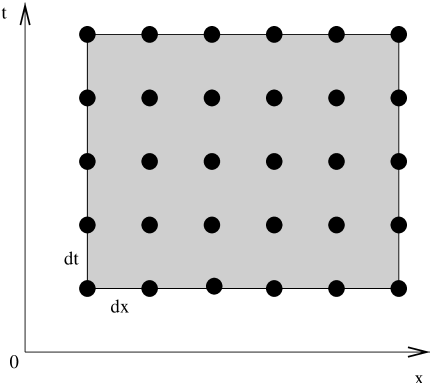
Figure 7: A 2-dimensional grid with constant spacing. We note that the domain does not have to be rectangular and different values for $dt$ and $dx$ may be used.

without abandoning the concept of a uniform grid.
For the presentation of finite difference expressions it is convenient to introduce a short hand notation for the function values at the grid points. For this purpose we define $f_{k}^{n}:=f(x_{k},t_{n})$. If the meaning is obvious we may omit either index.

2.3.2 Derivatives and finite differences

We describe the approximation of derivatives with finite differences in the case of spatial derivatives. The same ideas apply to time derivatives. Suppose a function $f$ is given at positions $x_{0},\ldots,x_{K}$ for fixed time and we want to calculate $\displaystyle{\frac{\partial^{m}f}{\partial x^{m}}}$ at $x_{k}$. For this purpose we expand $f$ in a Taylor series about $x_{k}$ which allows us to express $f_{k}$, $f_{k-1}$, $f_{k+1}$,$\ldots$ in terms of $f$ and its derivatives at $x_{k}$. Next the derivative that needs to be calculated is expressed as a linear combination of the function values at neighbouring grid points. The required finite difference expression is then obtained from inserting the Taylor expansions for the $f_{k}$, $f_{k-1}$, $f_{k+1},\ldots$ and comparing the coefficients on both sides of the equations. The number of grid points that needs to be included in this calculation depends on the degree of the derivative and the order of accuracy to be achieved.
We illustrate these ideas by calculating the second derivative $f_{k}^{\prime\prime}$ with second order accuracy. We assume that the function $f$ is known at the grid points $x_{k}$, $x_{k-1}$, $x_{k-2}$ and $x_{k-3}$. By Taylor expanding $f$ around $x_{k}$ we can relate the function values to $f$ and its derivatives at $x_{k}$

$$f_{k} =f_{k},$$ (2.63)

$$f_{k-1} =f_{k}-f_{k}^{\prime}dx+\frac{1}{2}f_{k}^{\prime\prime}dx^{2}-\frac{1}{6}f_{k}^{\prime\prime\prime}dx^{3}+\mathscr{O}(dx^{4}),$$ (2.64)

$$f_{k-2} =f_{k}-f_{k}^{\prime}2dx+\frac{1}{2}f_{k}^{\prime\prime}4dx^{2}-\frac{1}{6}f_{k}^{\prime\prime\prime}8dx^{3}+\mathscr{O}(dx^{4}),$$ (2.65)

$$f_{k-3} =f_{k}-f_{k}^{\prime}3dx+\frac{1}{2}f_{k}^{\prime\prime}9dx^{2}-\frac{1}{6}f_{k}^{\prime\prime\prime}27dx^{2}+\mathscr{O}(dx^{4}).$$ (2.66)

Next we write $f_{k}^{\prime\prime}$ as a linear combination of the function values

$$dx^{2}\cdot f_{k}^{\prime\prime} =Af_{k}+Bf_{k-1}+Cf_{k-2}+Df_{k-3}.$$ (2.67)

If we insert Eqs. (2.63)-(2.66) for the function values $f_{k-3},\ldots,f_{k}$ and compare the coefficients of both sides of the equation, we obtain the system of linear equations

$$\begin{split}A+B+C+D&=0,\\ B+2C+3D&=0,\\ B+4C+9D&=2,\\ B+8C+27D&=0.\end{split}$$ (2.68)

The solution is $A=2$, $B=-5$, $C=4$, $D=-1$ and we can approximate the derivative $f_{k}^{\prime\prime}$ with second order accuracy by

$$f_{k}^{\prime\prime} =\frac{2f_{k}-5f_{k-1}+4f_{k-2}-f_{k-3}}{dx^{2}}+\mathscr{O}(dx^{2}).$$ (2.69)

In general, a one sided calculation as used in this example yields less accurate estimates of the derivative and two sided approximations are to be preferred. In our case the centred finite difference expression is given by

$$f_{k}^{\prime\prime} =\frac{f_{k+1}-2f_{k}+f_{k-1}}{dx^{2}}+\mathscr{O}(dx^{2}).$$ (2.70)

If we substitute expressions corresponding to (2.69) or (2.70) for all derivatives, the differential equation is replaced by a large set of algebraic equations.

2.3.3 The leapfrog scheme

The leapfrog scheme is a second order in space and time finite differencing scheme in which three successive time-levels are used at each integration step. If we assume that the differential equation can be written in the form

$$f_{,t} =H(f,f_{,x},f_{,xx},...,x,t),$$ (2.71)

the right hand side can be evaluated on the $n^{th}$ time slice. The time derivative, on the other hand, is approximated by

$$\frac{\partial f}{\partial t} =\frac{f^{n+1}-f^{n-1}}{2dt},$$ (2.72)

and the difference equation can be explicitly solved for $f^{n+1}$. Because of the centred finite difference approximation for $f_{,t}$, three time slices are involved in the calculation. As an example

Figure 8: The leapfrog scheme: In the evolution one slice is leapt over.

we consider the special case where $H=f_{,x}$. At the spatial position $x_{k}$ the finite difference equation is then given by

$$f^{n+1}_{k} =f^{n-1}_{k}+\frac{dt}{dx}(f^{n}_{k+1}-f^{n}_{k-1}).$$ (2.73)

The value of $f$ is taken on slice $n-1$ and we “leap” across slice $n$ to calculate $f^{n+1}$. This property is schematically illustrated in Fig. 8 and has given the scheme its characteristic name. The need to store the function values of two time slices makes this scheme more memory intensive than 2-level schemes such as the McCormack scheme discussed in the next section. Second order accurate two-level schemes, on the other hand, involve more complicated finite difference expressions and are therefore more CPU-intensive.
A potential problem of the leap-frog scheme is its vulnerability to the so-called mesh-drifting effect, an instability that results from the decoupling of odd and even mesh points. This instability can often be cured by evolving some of the variables on a separate grid translated with respect to the original one by half a grid step (staggered leap-frog) or introducing artificial dissipation which couples odd and even grid points. In our application of this scheme in section 3, however, we do not encounter this problem and have no need to use either of the remedies.
We finally note that in Eq. (2.73) the function value on the new slice $f^{n+1}_{k}$ is expressed explicitly in terms of known function values on previous slices. Finite differencing schemes with this property are called explicit schemes. In section 2.3.6 we will, by contrast, introduce an implicit scheme where this is in general not possible for non-linear partial differential equations and iterative methods or linear solvers are used to determine the $f^{n+1}_{k}$.

2.3.4 The McCormack scheme

The McCormack scheme is another second order accurate explicit finite differencing method. In contrast to the leapfrog scheme it is a two-level method, i.e. requires storage of one previous slice only. However, this comes at the expense of two computation steps in the calculation of the new values, a predictor and a corrector step. We illustrate this method by considering the partial differential equation

$$f_{,t} =H(f,f_{,x},x,t).$$ (2.74)

In the first step preliminary values on the new time slice are calculated according to

$$\tilde{f}^{n+1}_{k} =f^{n}_{k}+\Delta t\cdot H^{n}_{k,k-1},$$ (2.75)

where $H^{n}_{k,k-1}$ is the source term evaluated to second order accuracy at $x_{k-1/2}$ by using $f^{n}_{k-1}$ and $f^{n}_{k}$. This predictor step itself is a first order accurate scheme, but the terms of first order truncation error are eliminated in the corrector step

$$f^{n+1}_{k} =f^{n}_{k}+\Delta t\cdot\frac{1}{2}\left(H^{n}_{k,k-1}+\tilde{H}^{n+1}_{k+1,k}\right),$$ (2.76)

where $\tilde{H}^{n+1}_{k+1,k}$ is the source term evaluated from the preliminary values $\tilde{f}^{n+1}_{k}$ and $\tilde{f}^{n+1}_{k+1}$. The extension to systems with more functions is obvious.

2.3.5 Relaxation

Relaxation is a method for solving so-called two point boundary value problems, that is ordinary differential equations (ODEs) where boundary conditions are given at different locations on the grid. A straightforward integration to obtain the solution is not possible in these cases and one needs to resort to more sophisticated techniques. One such technique, of which we will make extensive use in this work is numerical relaxation. In the case of ordinary differential equations only one independent coordinate is present which can be visualised in Fig. 7 by suppressing the time dimension so that we have only one row of grid points. It is straightforward to see that any ordinary differential equation can be written as a first order system. Without loss of generality we will therefore restrict our discussion to this case. Suppose for example that we have a system of 4 ODEs for 4 functions $A(x)$, $B(x)$, $C(x)$ and $D(x)$ given by

$$G_{i}(A,A_{,x},B,B_{,x},C,C_{,x},D,D_{,x}) =0,\qquad i=1\ldots 4.$$ (2.77)

A numerical solution consists of $4K$ function values $A_{1}$, $B_{1}$, $C_{1}$, $D_{1}$, $A_{2}$, $B_{2}$ and so on. It is convenient to introduce a vector $f_{j}$ to label these values, i.e. $f_{1}:=A_{1}$, $f_{2}:=B_{1}$ and so on. For each pair of grid points $k$, $k-1$ we apply centred finite differencing according to

$$A =\frac{1}{2}(A_{k}+A_{k-1}),$$ (2.78)

$$A_{,x} =\frac{A_{k}-A_{k-1}}{\Delta x},$$ (2.79)

and likewise for the other functions. In combination with Eq. (2.77) this amounts up to $4(K-1)$ algebraic equations for the 4K variables $f_{j}$. This set is completed by 4 boundary conditions for $A$, $B$, $C$ and $D$ and we arrive at 4K algebraic equations which we write in the form

$$F_{i}(f_{j}) =0.$$ (2.80)

In general these equations are non-linear and we have to resort to iterative techniques to obtain a solution $f_{j}$. For this purpose we assume that $f_{j}$ is a solution of (2.80) and $f^{0}_{j}$ is a sufficiently close guess. Then $4K$-dimensional Taylor expansion yields

$$0 =F_{i}(f_{j})\approx F_{i}(f^{0}_{j})+\sum_{j}{\frac{\partial F_{i}}{\partial f_{j}}\Delta f_{j}},$$ (2.81)

where $\Delta f_{j}=f_{j}-f^{0}_{j}$. This is simply a system of linear equations which we can write as

$${\bf A}\Delta{\bf f}={\bf b},$$ (2.82)

where

$${\bf A}_{ij}=\frac{\partial F_{i}}{\partial f_{j}},$$ (2.83)

$${\bf b}_{i}=-F_{i}(f^{0}_{j}).$$ (2.84)

Even though the Jacobi matrix A is a $4K$ by $4K$ matrix, it is a sparse matrix which greatly simplifies its inversion. If the equations $F_{i}=0$ are ordered appropriately, A has block diagonal structure and can be inverted by standard methods (see for example Press1989). Starting with an initial guess $f^{0}_{j}$, we can calculate the correction $\Delta f_{j}$ which leads to an improved approximation $f^{1}_{j}$ and the process is repeated until the norm $||\Delta f_{j}||$ satisfies some convergence criterion. This iteration scheme is the Newton-Raphson method generalized to $4K$ dimensions and usually converges fast.

2.3.6 The Crank-Nicholson scheme

The Crank-Nicholson scheme is a two-level evolution scheme for partial differential equations and can be considered a generalization of the relaxation scheme. Again the system of equations is rewritten as a first order system by introducing auxiliary variables. For convenience we will illustrate the scheme for one equation and one function $f$ only. The extension to more functions is obvious. Consider the PDE

$$G(f,f_{,t},f_{,x},x,t) =0$$ (2.85)

on a grid of the type shown in Fig. 7 with $K$ points on each slice $t={\rm const}$. We can use a stencil of the type shown in Fig. 9 to obtain second order centred finite

Figure 9: The numerical stencil used in the Crank Nicholson scheme to obtain centred second order accurate expressions for $f$, $f_{,x}$ and $f_{,t}$ at position $(x_{k}+\Delta x/2,t^{n}+\Delta t/2)$.

difference expressions for the functions and their derivatives according to

$$f =\frac{1}{4}(f^{n+1}_{k}+f^{n+1}_{k-1}+f^{n}_{k}+f^{n}_{k-1}),$$ (2.86)

$$f_{,x} =\frac{f^{n+1}_{k}-f^{n+1}_{k-1}+f^{n}_{k}-f^{n}_{k-1}}{2\Delta x},$$ (2.87)

$$f_{,t} =\frac{f^{n+1}_{k}+f^{n+1}_{k-1}-f^{n}_{k}-f^{n}_{k-1}}{2\Delta t}.$$ (2.88)

Inserting these relations into Eq. (2.85) we obtain $K-1$ algebraic equations for the $K$ unknown values $f^{n+1}_{k}$ in terms of the known $f^{n}_{k}$. The set is completed by the boundary condition for $f$ and we are in exactly the same situation as in Eq. (2.80) in the relaxation scheme. Note that each algebraic equation involves two unknown values $f^{n+1}_{k}$, $f^{n+1}_{k-1}$, so it is in general not possible to obtain explicit expressions similar to Eq. (2.73) in the leapfrog-scheme. Therefore methods like the Crank-Nicholson scheme are called implicit and a solution is obtained by using iterative methods. The initial guess for the values on the new slice is usually taken from the previous slice.
An explicit variation of the Crank-Nicholson scheme which has attracted a good deal of attention recently is the so-called iterative Crank-Nicholson method. There one calculates intermediate values $\tilde{u}^{n+1}$ on the new time slice according to the unconditionally unstable forward time centred space method and averages these values with the data on the old slice $n$ to obtain $\bar{u}^{n+1/2}=(\tilde{u}^{n+1}+u^{n})/2$. These averaged values are then used to calculate the source terms in the partial differential equation at time $t^{n+1/2}$ and can be used to evolve the data with centred finite differencing of the time derivatives in a second order scheme. In fact this iteration process can be repeated arbitrarily often and the number of iterations significantly affects the stability properties of the scheme. In particular Teukolsky2000 has shown that the smallest number of iterations required for a stable method is two and that any further iterations do not lead to any superior performance in terms of stability and accuracy.
Before we apply these numerical schemes to general relativistic scenarios, we discuss some general properties of numerical evolution schemes.

2.3.7 Consistency

If we take the difference equations and calculate the $f_{k}^{n}$ as a Taylor series about some fixed grid-point, we will again arrive at a differential equation for $f$. The difference between this differential equation and the original one is the truncation error. The numerical scheme is said to be consistent if the truncation error vanishes in the limit $dx,dt\rightarrow 0$ (see for example LeVeque1992). Assuming that $dx$ and $dt$ differ by a constant factor in the limit $dx\to 0$, the scheme is of $n^{th}$ order accuracy if the leading term of the truncation error vanishes as $dx^{n}$.

2.3.8 Stability

The concept of stability is concerned with an exponentially increasing deviation of the numerical solution from the solution of the underlying differential equation. If such a deviation is present either due to the initial data or round off errors, it will quickly swamp the entire numerical solution and make the code practically useless. The stability of a code can depend on many properties. Often changing the grid parameters $dx$, $dt$ has a substantial effect on the stability.
In the case of linear partial differential equations one can use the von Neumann stability analysis in order to test finite differencing schemes for stability. For this purpose we assume that the numerical grid is uniform, i.e. $dx$ and $dt$ are constant. The solution of the difference equation can then be expanded as a Fourier series

$$f^{n}(x) =\sum_{{\kappa}}\hat{f}^{n}(\kappa)e^{i\kappa x},$$ (2.89)

where $\kappa$ is a spatial wave vector (1-dimensional in our case). It is sufficient to consider one mode $\hat{f}^{n}(\kappa)e^{i{\kappa}x}$ which can be written as

$$\hat{f}^{n}_{{\kappa}} =\xi({\kappa})^{n}e^{i{\kappa}x},$$ (2.90)

if the coefficients of the difference equations show sufficiently weak variation in space and time and can be considered nearly constant. The important aspect is that the amplitude at some time is obtained from that of the preceding time step by multiplication with a time independent factor $\xi({\kappa})$. If $|\xi({\kappa})|>1$ the scheme is unstable. In practice, Eq. (2.90) is inserted into the difference equations which then is solved for $\xi$. For many applications, the result is the well known Courant-Friedrichs-Lewy condition (CFL-condition)

$$\left|\frac{\lambda_{i}\cdot dt}{dx}\right|\leq 1,$$ (2.91)

where the $\lambda_{i}$ are the slopes of the characteristics of the underlying system of PDEs. An intuitive interpretation of this result is that the numerical domain of dependency of the point where $f$ is to be calculated must contain the physical one. Indeed this condition was recognised as a necessary stability condition for any numerical scheme by Courant1928 (See Courant1967 for an English translation). The CFL condition is therefore commonly used in non-linear codes to determine the permissible Courant factor $dt/dx$. We will illustrate the use of this criterion in the evolution of non-linear radial oscillations of neutron stars in section 5.3.5.

2.3.9 Convergence

It is necessary to carefully distinguish between consistency, stability and convergence of a code. The convergence of a numerical method is a stronger requirement than consistency or stability. It is quite obvious, for example that a consistent method will not be convergent if it is unstable. In order to define convergence, we consider a solution $f$ of the system of differential equations and a solution $F$ of the corresponding difference equations. We note that $F$ is never obtained in practice due to round off errors. A scheme is said to converge if

$$|f_{k}^{n}-F_{k}^{n}|\rightarrow 0\qquad{\rm as}\qquad dx,dt\rightarrow 0.$$ (2.92)

In the case of linear equations convergence can be ensured by the Lax Equivalence Theorem which states: Given a properly posed linear initial value problem and a finite difference approximation to it that satisfies the consistency condition, the stability is a necessary and sufficient condition for convergence (see for example Richtmyer1967).
In the case of non-linear equations there is no corresponding theorem but in some cases we will be able to check our codes for convergence by comparing the results with known analytic solutions. If such analytic solutions are not available, we need to use reference solutions obtained for high resolutions instead. We will thus be able to ensure the Cauchy convergence of the numerical scheme. This is, however, a weaker statement than Eq. (2.92) and does not strictly guarantee convergence to the solution of the differential equations.

3 Cauchy characteristic matching in cylindrical symmetry

3.1 The idea of Cauchy characteristic matching

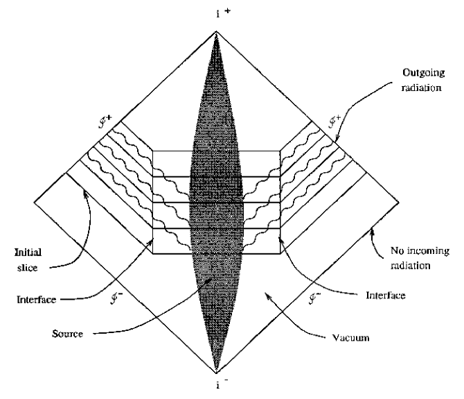
Figure 10: In this conformal diagram Cauchy characteristic matching is schematically illustrated. In the inner region matter is evolved with a “3+1” scheme whereas characteristic coordinates defined by the null geodesics are used in the outer vacuum region. The two formalisms are matched at the interface at finite radius.

Cauchy characteristic matching (CCM) is a method that simultaneously makes use of the beneficial properties of the “3+1” and the characteristic formalism. In section 2.1 we have seen that in the “3+1” case spacetime is decomposed into 3-dimensional space-like hypersurfaces threaded by a one parameter family of curves. The dynamic variables are the components $\hbox{\grvec g}_{ij}$ of the 3-metric of the hypersurfaces. A complete set of initial data consists of values for $\hbox{\grvec g}_{ij}$ and their time derivatives on some initial hypersurface. The second order evolution equations then determine the 4-metric of the spacetime up to gauge transformations. This type of initial value problem is known as a Cauchy problem and has been extensively used for the numerical solution of Einstein’s field equations. It is however not suitable for the analysis of gravitational radiation since it is not clear how to incorporate null infinity into a finite numerical grid via conformal compactification. Instead one uses approximating techniques to extract information about the gravitational radiation at finite radii and imposes outgoing radiation boundary conditions in order to prevent incoming gravitational waves. Unfortunately attempts to implement these boundary conditions give rise to spurious reflected numerical waves. Characteristic formalisms solve this problem in an elegant way. Spacetime is decomposed into a 2-parameter family of 2-dimensional space-like surfaces threaded by two 1-parameter families of curves. At least one of these families consists of null geodesics, the characteristics of the propagation of radiation. The spacetime can be compactified by standard methods, exact boundary conditions can be applied at future or past null infinity and gravitational radiation can be properly analysed. In regions of strong curvature, however, caustics can form and the foliation along null geodesics breaks down.
A possible remedy for this problem consists in using both a “3+1” and a characteristic formulation, each in its preferred region. Normally an astrophysical scenario is approximated as a finite inner region containing all the matter (a neutron star, for example) and the outer vacuum region with an observer located at future null infinity. In CCM a “3+1” scheme is used for the evolution of the interior and a characteristic formulation for the evolution of the exterior region. At a finite radius an interface facilitates the transfer of information between these two regions. The method is illustrated in Fig. 10 where the dark shaded area represents the astrophysical source. Gravitational waves emitted from this source travel along null geodesics which are given by straight lines at an angle of 45 degrees in this figure. In the outer region the null geodesics are used to define the characteristic coordinate axis.
The feasibility of combining Cauchy algorithms with characteristic methods in order to evolve the gravitational field was first studied by Bishop1992. The first attempts at obtaining numerical evolutions have been carried out in one spatial dimension. The work of the Southampton CCM-group in cylindrical symmetry will be discussed in detail in the next section. The Pittsburgh relativity group studied CCM in spherical symmetry by evolving the Einstein-Klein-Gordon system (Gomez1996). They have demonstrated second order convergence and found no indications of back reflection or instabilities at the interface. After the demonstration of the viability of CCM in one dimension attention shifted towards higher-dimensional problems. The Southampton relativity group focused their studies on the axisymmetric case. After laying the theoretical foundations (dInverno1996, dInverno1997) a great deal of work has gone into the development of an axisymmetric CCM code (see Pollney2000 for details). This code has now been completed and is currently being evaluated and tested. In contrast the Pittsburgh group has immediately turned their attention towards the general 3-dimensional case. Bishop1996 and Bishop1997 have probed the use of Cauchy-characteristic matching in three dimensions by evolving non-linear scalar waves in a flat space-time. The application of these ideas to 3-dimensional problems in general relativity has resulted in a module for the combination of Cauchy and characteristic codes for the evolution of a binary black hole (Bishop1998). A more comprehensive overview of the ongoing research using Cauchy-characteristic matching can be found in Winicour2001.

3.2 The Southampton CCM-project

The Southampton CCM-project is a long term project devoted to the study of Cauchy-charac-teristic matching in scenarios of decreasing symmetry assumptions (dInverno2000). The first step was to demonstrate the viability of the approach. That was done by Clarke1994 by evolving the wave equation in flat spacetime. Attention then turned towards gravitational waves in cylindrical symmetry. The theoretical foundations were laid by Clarke1995 and the resulting code of Dubal1995 showed good agreement with analytic solutions containing one gravitational degree of freedom. Furthermore Dubal1995 demonstrated the superior performance of the CCM-method as compared with the use of artificial outer boundary conditions in “3+1” schemes. dInverno2000b presented a generalisation of this code to also include the rotational degree of freedom. They find, however, that the convergence of the code drops to first order level in later stages of the evolutions. In this work we will present a new code that allows us to include the rotational degree of freedom in terms of natural geometrical variables with regular behaviour at null infinity. This reformulation resulted in improved accuracy, long term stability and ensures second order convergence over long evolution times. We will demonstrate the improved quality by comparing the numerical results with analytic solutions possessing both gravitational degrees of freedom.
The Southampton CCM-project has continued meanwhile with the development of the axisymmetric code mentioned in the previous section.

3.3 The original code

In this section we will describe the cylindrically symmetric Cauchy characteristic matching code developed by the Southampton Relativity Group (Clarke1995, Dubal1995). This code was used to reproduce the analytic solution by Weber1957, which possesses one gravitational degree of freedom, with high accuracy and second order convergence. dInverno2000b presented an extension of this code based on the formulation of Clarke1995 to also include the rotational degree of freedom. Their difficulties in obtaining a long term stable second order convergent code motivated the reinvestigation of the problem described in this thesis.
In their derivation of the equations Clarke1995 find it necessary to decompose spacetime according to the methods of Geroch1970 in order to eliminate irregularities of the equations in the characteristic region. The Geroch decomposition plays a crucial role in our reformulation and will also be used in section 4 when we numerically simulate cosmic strings. Before we turn our attention to the cylindrically symmetric CCM code, we will therefore describe the Geroch decomposition in more detail.

3.3.1 The Geroch decomposition

A problem generally faced in cylindrical symmetry is that the spacetime is not asymptotically flat due to the infinite extension in the $z$-direction. The decomposition of Geroch1970 solves this problem by factoring out the Killing direction and reformulating the 4-dimensional problem in terms of two scalar fields on an asymptotically flat 3-dimensional spacetime. Suppose, the spacetime admits a Killing field $\hbox{\grvec x}^{\mu}$ which in the case of cylindrical symmetry simply is $\mathchoice{{\hbox{\boldmath$\displaystyle\partial$}}}{{\hbox{\boldmath$\textstyle\partial$}}}{{\hbox{\boldmath$\scriptstyle\partial$}}}{{\hbox{\boldmath$\scriptscriptstyle\partial$}}}_{z}$. Then we define the norm of the Killing vector

$$\nu =\hbox{\grvec x}^{\alpha}\hbox{\grvec x}_{\alpha},$$ (3.1)

and the Geroch twist

$$\hbox{\grvec t}_{\alpha} =-\hbox{\grvec e}_{\alpha\beta\rho\sigma}\hbox{\grvec x}^{\beta}\nabla^{\rho}\hbox{\grvec x}^{\sigma},$$ (3.2)

where $\hbox{\grvec e}_{\alpha\beta\rho\sigma}$ is the completely antisymmetric Levi-Cevita tensor. These fields are well defined on the 3-dimensional space $\mathcal{S}$ given by $z=\mathrm{const}$ with the resulting metric

$$\hbox{\vec h}_{\alpha\beta} =\hbox{\vec g}_{\alpha\beta}-\frac{1}{\nu}\hbox{\grvec x}_{\alpha}\hbox{\grvec x}_{\beta}.$$ (3.3)

If $D_{\mu}$ denotes the covariant derivative associated with the 3-metric h, one can show that

$$D_{[\rho}\hbox{\grvec t}_{\sigma]} =\hbox{\grvec e}_{\rho\sigma\alpha\beta}\hbox{\grvec x}^{\alpha}\hbox{\vec R}^{\beta}_{\,\,\,\lambda}\hbox{\grvec x}^{\lambda}.$$ (3.4)

In vacuum the right hand side vanishes so that $\hbox{\grvec t}_{\sigma}$ is curl free and can be expressed in terms of a potential

$$\hbox{\grvec t}_{\sigma} =D_{\sigma}\tau.$$ (3.5)

It is a remarkable fact that the right hand side of Eq. (3.4) will also vanish in some non-vacuum cases. In the discussion of cosmic strings in section 4 we will encounter such an example.
Geroch has then shown that the Einstein equations for the metric g of the 4-dimensional spacetime can be written in terms of the two scalar fields $\tau$ and $\nu$ and the 3-metric h

$${\cal R}_{ab} = \frac{1}{2}\nu^{-2}[(D_{a}\tau)(D_{b}\tau)-\hbox{\vec h}_{ab}(D_{m}\tau)(D^{m}\tau)]+\frac{1}{2}\nu^{-1}D_{a}D_{b}\nu-\frac{1}{4}\nu^{-2}(D_{a}\nu)(D_{b}\nu)$$ (3.6)

$$+8\pi\hbox{\vec h}_{a}{}^{\alpha}\hbox{\vec h}_{b}{}^{\beta}(\hbox{\vec T}_{\alpha\beta}-\frac{1}{2}\hbox{\vec g}_{\alpha\beta}\hbox{\vec T}),$$

$$D^{2}\nu = \frac{1}{2}\nu^{-1}(D_{m}\nu)(D^{m}\nu)-\nu^{-1}(D_{m}\tau)(D^{m}\tau)+16\pi(\hbox{\vec T}_{\alpha\beta}-\frac{1}{2}\hbox{\vec g}_{\alpha\beta}\hbox{\vec T})\hbox{\grvec x}^{\alpha}\hbox{\grvec x}^{\beta},$$ (3.7)

$$D^{2}\tau = \frac{3}{2}\nu^{-1}(D_{m}\tau)(D^{m}\nu),$$ (3.8)

where Latin indices run from 0 to 2 and $\mathcal{R}_{ab}$ is the Ricci tensor associated with the 3-metric h. Note that even in the case of a vanishing energy-momentum tensor T, the scalar fields $\nu$ and $\tau$ present source terms in the field equations (3.6) for the 3-metric h.
In the vacuum case $\hbox{\vec T}_{\alpha\beta}=0$, Sjodin2000 have shown how it is possible to reformulate the Einstein-Hilbert Lagrangian in terms of $\nu$, $\tau$ and the conformal 3-metric $\tilde{\hbox{\vec h}}_{ab}=\nu\hbox{\vec h}_{ab}$. This leads directly to the 3-dimensional energy-momentum tensor

$$\mathcal{T}_{ab}=\frac{1}{2}\nu^{-2}[{\tilde{D}}_{a}\tau{\tilde{D}_{b}}\tau-\frac{1}{2}\tilde{\hbox{\vec h}}_{ab}\tilde{\hbox{\vec h}}^{cd}(\tilde{D}_{c}\tau)(\tilde{D}_{d}\tau)+{\tilde{D}}_{a}\nu{\tilde{D}_{b}}\nu-\frac{1}{2}\tilde{\hbox{\vec h}}_{ab}\tilde{\hbox{\vec h}}^{cd}(\tilde{D}_{c}\nu)(\tilde{D}_{d}\nu)],$$ (3.9)

where $\tilde{D}_{a}$ is the covariant derivative associated with the conformal 3-metric $\tilde{\hbox{\vec h}}$. Since the Weyl-curvature vanishes identically in three dimensions, the curvature is completely determined by the Ricci tensor $\mathcal{R}_{ab}$, i.e. the energy-momentum tensor $\mathcal{T}_{ab}$ which in turn is determined by $\nu$ and $\tau$. Thus the gravitational degrees of freedom of the original 4-dimensional spacetime are represented by the scalar fields $\nu$ and $\tau$. If matter is present in the 4-dimensional spacetime, there are extra terms on the right hand side of (3.9).

3.3.2 The equations of the original code

We will now turn our attention to the original cylindrically symmetric CCM code of the Southampton relativity group. An extensive description of this code and the derivation of the equations can be found in Clarke1995 and Dubal1995. In order to illustrate the effects of our reformulation, we will include here a rather detailed description of their equations and choice of variables. They start with the metric in Jordan, Ehlers, Kundt and Kompaneets (JEKK) form (Jordan1960, Kompaneets1958)

$$ds^{2} =e^{2(\gamma-\psi)}(-dt^{2}+dr^{2})+r^{2}e^{-2\psi}d\phi^{2}+e^{2\psi}(\omega d\phi+dz)^{2},$$ (3.10)

which describes a general cylindrically symmetric vacuum spacetime. The metric functions $\psi$, $\omega$ and $\gamma$ are functions of $(r,t)$ only. In terms of the gauge freedom discussed in section 2.1.2 this choice implies a vanishing shift vector and the lapse is determined by the requirement that $\hbox{\vec g}_{tt}=-\hbox{\vec g}_{rr}$. As a consequence the null geodesics are given by the simple relations $t\pm r=\mathrm{const}$. In the outer characteristic region, the line element is rewritten by transforming to the coordinates

$$u =t-r,$$ (3.11)

$$y =\frac{1}{\sqrt{r}},$$ (3.12)

and the regions are matched at $r=1=y$. Clarke1995 find, however, that the compactified field equations cannot be made regular in this way. Therefore they factor out the $z$-direction in the outer region according to the Geroch decomposition described above. This leads to a reformulation of the problem in terms of the variables

$$m =\frac{\nu-1}{y},$$ (3.13)

$$w =\frac{\tau}{y},$$ (3.14)

where $\tau$ is the Geroch potential and $\nu$ the norm of the $z$-Killing vector. These are related to the metric functions $\psi$ and $\omega$ by Eqs. (3.1) and (3.2) which in this particular case become

$$\nu =e^{2\psi},$$ (3.15)

$$\tau_{,y} =y^{2}e^{4\psi}\omega_{,u}.$$ (3.16)

With this choice of variables one obtains two evolution equations for $\psi$ and $\omega$ in the interior Cauchy region and a constraint equation for $\gamma$. Dubal1995 write this set of equations as a first order system

$$\psi_{,t} =\frac{1}{r}\tilde{L},$$ (3.17)

$$\omega_{,t} =-2e^{-4\psi}L^{\phi}_{z},$$ (3.18)

$$\tilde{L}_{,t} =\frac{1}{r}[r^{2}\psi_{,rr}+r\psi_{,r}-\frac{1}{2}e^{4\psi}\omega^{2}_{,r}+2e^{-4\psi}(L^{\phi}_{z})^{2}],$$ (3.19)

$$L^{\phi}_{z,t} =\frac{1}{r}e^{4\psi}(\frac{1}{2}\omega_{,r}-\frac{1}{2}r\omega_{,rr}-2r\psi_{,r}\omega_{,r}),$$ (3.20)

$$\chi_{,r} =\frac{1}{4r}e^{4\psi}\omega^{2}_{,r}-\psi_{,r}+r\psi^{2}_{,r}+\frac{1}{r}[\tilde{L}^{2}+e^{-4\psi}(L^{\phi}_{z})^{2}],$$ (3.21)

where $\chi=\gamma-\psi$. The corresponding set of equations in the characteristic region is given by two evolution equations for $m$ and $w$ and a hypersurface equation for $\gamma$ which is again written as a first order system

$$m_{,u}=\,\, \nu M,$$ (3.22)

$$w_{,u}=\,\, \nu W,$$ (3.23)

$$\begin{split}M_{,y}=&-\frac{1}{\nu}(yw)_{,}{y}W+\frac{1}{4\nu}\biggl{[}-y(m+y^{2}m_{,yy}+3ym_{,y})\\[10.0pt] &+\frac{1}{\nu}y^{2}(m^{2}+2ymm_{,y}-w^{2}-2yww_{,y}+y^{2}m^{2}_{,y}-y^{2}w^{2}_{,y})\biggr{]},\end{split}$$ (3.24)

$$\begin{split}W_{,y}=\,\,&\frac{1}{\nu}(yw)_{,y}M+\frac{1}{4\nu}\biggl{[}-y(w+y^{2}w_{,yy}+3yw_{,y})\\[10.0pt] &+\frac{1}{\nu}2y^{2}(mw+ymw_{,y}+ywm_{,y}+y^{2}m_{,y}+y^{2}m_{,y}w_{,y})\biggr{]},\end{split}$$ (3.25)

$$\gamma_{,y}= -\frac{1}{8\nu^{2}}y[m^{2}+w^{2}+2y(mm_{,y}+ww_{,y})+y^{2}(m^{2}_{,y}+w^{2}_{,y})].$$ (3.26)

The transformation between the two pairs of variables $(\psi,\omega)$ and $(m,w)$ and their derivatives is implemented at the interface at $r=1=y$ according to the relations

$$\tilde{L} = \frac{M}{2y},$$ (3.27)

$$\omega_{,r} = \frac{W}{y\nu},$$ (3.28)

$$m = \frac{1}{y}(e^{2\psi}-1),$$ (3.29)

$$(yw)_{,y} = -\frac{2}{r}L_{z}^{\phi}.$$ (3.30)

The problematic relations are (3.28) and (3.30) which involve the spatial derivative of $\omega$ and $w$. The presence of spatial derivatives in combination with the interpolation techniques applied at the interface make the implementation of these relations a rather subtle issue.
The code of Dubal1995 formed the starting point for our investigation of the problem. This code has been well checked in the non-rotating case but did not include the implementation of Eqs. (3.28) and (3.30) for the rotational variables $\omega$ and $w$ at the interface. In this work we therefore started with the addition of these missing modules to the original code. In order to describe our implementation it is necessary to first discuss the numerical techniques, in particular those underlying the transmission of information from the Cauchy to the characteristic region and vice versa.

3.3.3 The numerical implementation

We will now discuss the numerical implementation of Eqs. (3.17)-(3.30). The numerical grid used for the evolution consists of an inner Cauchy region which covers the range $0\leq r\leq 1$ and the outer characteristic region extending from $r=1$ to infinity which corresponds to the range $1\geq y\geq 0$. The evolution equations in these regions are discretized in a straightforward way using the leapfrog scheme described in section 2.3.3 while second order centered finite differencing is used for the constraints. If we assume that all functions are known on the time slices $n$, $n-1$ and $n-2$, a full evolution cycle consists of the following steps.

• Evolution of $\psi$, $\omega$, $\tilde{L}$ and $L_{z}^{\phi}$ at the interior grid points of the Cauchy region according to Eqs. (3.17)-(3.20).

• Update of these variables at the origin according to the inner boundary conditions $\psi_{,r}=\omega_{,r}=\tilde{L}_{,r}=L^{\phi}_{z,r}=0$.

• Evolution of $\psi$ and $\omega$ at the outer boundary of the Cauchy grid ($r=1$) according to Eqs. (3.17), (3.18).

• Extraction of $\psi$ and $\omega$ from the interface at $1+dr$ on the Cauchy grid on time slice $n$.

• Evolution of $\tilde{L}$, $L_{z}^{\phi}$ at the outer boundary of the Cauchy grid ($r=1$) according to Eqs. (3.19), (3.20).

• Calculation of $\chi$ on the Cauchy grid via quadrature according to Eq. (3.21).

• Evolution of $m$ and $w$ in the characteristic region according to Eqs. (3.22), (3.23).

• Extraction of $m$ and $w$ from the interface at $1+dy$ on the characteristic grid on time slice $n+1$.

• Calculation of $M$, $W$ and $\gamma$ on the characteristic grid via quadrature according to Eqs. (3.24)-(3.26).

The crucial steps which provide the flow of information through the interface are (4) and (8). These steps together with the start up procedure required to get the leap-frog scheme running will now be discussed in more detail. We start with the interface.
We first note that the interface is fixed at the radial position $r=1=y$. Since we always have the freedom to rescale the radial coordinate $r$ by a constant factor, this implies no loss of generality. From a numerical point of view the need of an interface arises from the calculation of spatial derivatives at $r=1$ on the Cauchy grid and $y=1$ on the characteristic grid. The centred finite differencing used for the leapfrog scheme as illustrated in Eq. (2.73) requires knowledge of the Cauchy variables at $r=1+dr$ and the characteristic variables at $y=1+dy$ for this purpose. In order to obtain these values, they need to be calculated with interpolation techniques using Eqs. (3.27)-(3.30). We will describe this process in the case of the direction “char$\rightarrow$Cauchy” corresponding to step (4). The reverse direction in step (8) works in complete analogy. The situation is graphically illustrated in Fig. 11.

Figure 11: The interface in the direction from the characteristic to the Cauchy region. See the text for details.

The derivatives of a function $f$ at $r=1$ can be calculated to second order accuracy by centred finite differencing

$$f_{,r}|_{K} =\frac{f_{K+1}-f_{K-1}}{2dr},$$ (3.31)

$$f_{,rr}|_{K} =\frac{f_{K+1}-2f_{K}+f_{K-1}}{dr^{2}},$$ (3.32)

if $f_{K+1}$ is obtained from interpolation to fourth order accuracy in the characteristic region. For this purpose $\psi$, $\omega_{,r}$, $\tilde{L}$ and $L^{\phi}_{z}$ are calculated in terms of the characteristic variables according to Eqs. (3.27)-(3.30) at the 12 points of the characteristic region (including 3 points at the interface) indicated by filled circles in Fig. 11. These values can then be used to obtain the function values $\psi_{K+1}$ and $\omega_{K+1}$ at location $r_{K+1}$ with the required accuracy.
An alternative to this method consists in using the same interpolation technique to calculate the $r$-derivatives $\psi_{,r}$ and $\omega_{,r}$ at grid point $K+1$ instead of the function values $\psi$ and $\omega$. We can then calculate the $r$-derivatives at the interface from

$$f_{,r}|_{K} =\frac{f_{,r}|_{K+1}+f_{,r}|_{K-1}}{2},$$ (3.33)

$$f_{,rr}|_{K} =\frac{f_{,r}|_{K+1}-f_{,r}|_{K-1}}{2dr}.$$ (3.34)

Even though this alternative looks natural for the transformation between $\omega$ and $w$ because these variables are related via their derivatives according to Eq. (3.28), it does not lead to any improvement of the performance of the code.
The second point we need to discuss is the so-called start-up problem. It is an intrinsic difficulty of 3-level schemes such as the leap-frog algorithm that the specification of initial data on one time slice will not be sufficient to start the numerical engine. Instead different techniques need to be used to obtain data on auxiliary time slices. Due to the requirements of the fourth-order interpolation at the interface we need information on two additional slices. The data on these auxiliary slices are calculated in three steps.

• The first order Euler scheme (see for example Press1989) is used to calculate data at $t=t_{0}-dt/2$.

• This auxiliary time slice is then used to determine the variables at $t=t_{0}-dt$ according to the leapfrog scheme.

• In another leapfrog step, this time using the full time step $dt$, data is calculated at $t_{0}-2dt$.

An alternative treatment at the interface is required for this start-up procedure, because the necessary three time-slices are not available at this stage. For this purpose the Cauchy grid is extended into the characteristic region by 10 grid points. The derivatives of the Cauchy variables can thus be calculated at $r=1$ using centred finite differencing and the derivatives of the characteristic variables follow from chain-rule. The treatment of the outer boundary of the Cauchy grid is irrelevant for the numerical evolution, since the spurious signal cannot travel across the additional 10 grid points during the three evolution steps at the start-up procedure and these points are not used in the remaining evolution.

3.3.4 Including the rotational degree of freedom $\omega$

In our first attempt to include the rotational degree of freedom we have made use of the set of variables of section 3.3.2, namely $\psi$, $\omega$ and $\chi$ in the inner and $m$, $w$ and $\gamma$ in the outer region. For this purpose we have extended the interface of the original code to also include the transformations between $\omega$ and $w$ as described in the previous section. In order to test the code we use the analytic solution from Xanthopoulos1986 which we will discuss in more detail in section 3.5.2. In Eqs. (3.55)-(3.68) we give analytic expressions for this solution in terms of the Killing vector $\nu$, the Geroch potential $\tau$ and the metric function $\gamma$. The corresponding results for the variables $\psi$, $m$ and $w$ are obtained straightforwardly from their definitions (3.13)-(3.15). The transformation into values for the function $\omega$ is more complicated. The result is given by Sjodin2000

$$\omega(t,r) =\sqrt{a^{2}+1}(X+Q-2)\frac{Z-Y}{2aZ},$$ (3.35)

where the auxiliary functions $Q$, $X$, $Y$ and $Z$ are defined in Eqs. (3.55)-(3.58). We have not been able, however, to obtain a long term stable evolution in this formulation of the problem. For 300 grid points in each region instability set in after less than 1000 time steps and from the pattern of the noise it is clear that the problems originate at the interface. In our attempts to overcome the instability we have varied the obvious parameters such as the Courant factor and the number of grid points over a large range, but no improvement has been achieved. We have also used the alternative implementation of the interface according to Eqs. (3.33), (3.34). Even though this alternative looks quite natural at least for the transformation between $\omega$ and $w$ which are related via their derivatives according to (3.28), we did not achieve a significantly better performance with this method. Finally we have changed the start time of the numerical evolution and, thus, the initial data. The obvious choice $t=0$ is not possible because some derivatives of Xanthopoulos’ solution are discontinuous at $t=0$, but any positive value large enough to ensure that the start-up procedure does not extend to negative times can be chosen. Again the code became unstable after less than 1000 time steps. We have therefore decided to restart the investigation of this problem by looking for alternative sets of variables.

3.4 A reformulation of the problem

A striking peculiarity of the formulation described above is the drastically different treatment of the Cauchy and the characteristic region. In view of the numerical subtleties associated with the interface one may question the wisdom of factoring out the $z$-direction in one region and work in the framework of the 4-dimensional spacetime in the other. It rather seems natural to look for as homogeneous a description of the whole spacetime as possible. In this context it is worth noting that the restriction of the Geroch decomposition to the characteristic region was a voluntary choice and not enforced at any stage of the derivation of the equations. We have therefore decided to factor out the $z$-direction in the Cauchy region as well and thus Geroch decomposed the whole spacetime. This enables us to use the same set of fundamental variables throughout spacetime and thus obtain almost trivial interface relations. A closer investigation of the equations suggests that aside from the metric function $\gamma$ the geometric variables $\nu$ and $\tau$ are the natural variables to describe the cylindrically symmetric spacetime. With this choice the equations in the Cauchy region can be written as

$$\nu_{,tt} =\frac{1}{\nu}(\nu_{,t}^{2}-\nu_{,r}^{2}+\tau_{,r}^{2}-\tau_{,t}^{2})+\nu_{,rr}+\frac{\nu_{,r}}{r},$$ (3.36)

$$\tau_{,tt} =\frac{2}{\nu}(\tau_{,t}\nu_{,t}-\tau_{,r}\nu_{,r})+\tau_{,rr}+\frac{1}{r}\tau_{,r},$$ (3.37)

$$\gamma_{,r} =\frac{r}{4\nu^{2}}(\nu_{,r}^{2}+\nu_{,t}^{2}+\tau_{,r}^{2}+\tau_{,t}^{2}).$$ (3.38)

In practice we use $\nu_{,t}$ and $\tau_{,t}$ as auxiliary variables in order to write Eqs. (3.36), (3.37) as a first order system. If we transform to the new set of variables the equations in the characteristic region become

$$\nu_{,u} =y\nu M,$$ (3.39)

$$\tau_{,u} =y\nu W,$$ (3.40)

$$M_{,y} =-\frac{y}{4\nu}\left[y\nu_{,yy}+\nu_{,y}+\frac{y}{\nu}(\tau_{,y}^{2}-\nu_{,y}^{2})\right]-W\frac{\tau_{,y}}{\nu},$$ (3.41)

$$W_{,y} =-\frac{y}{4\nu}\left(y\tau_{,yy}+\tau_{,y}-2\frac{y}{\nu}\nu_{,y}\right)+M\frac{\tau_{,y}}{\nu},$$ (3.42)

$$\gamma_{,y} =-\frac{y}{8\nu^{2}}(\tau_{,y}^{2}+\nu_{,y}^{2}).$$ (3.43)

Finally the non-trivial relations at the interface are now given by

$$\nu_{,t} =y\nu M,$$ (3.44)

$$\tau_{,t} =y\nu W.$$ (3.45)

We have developed a code using the numerical techniques of section 3.3.3 based on these evolution equations and interface relations.

3.5 Testing the code

In order to test the performance of the new code, we will check it against analytic solutions with one and two gravitational degrees of freedom. Furthermore we will demonstrate its internal consistency with a time dependent convergence analysis.
We have already mentioned the vacuum solution by Weber1957 that was successfully used by Dubal1995 to test their CCM code. A solution with both gravitational degrees of freedom was derived by Xanthopoulos1986. Both these solutions can be rewritten in terms of our variables $\nu$, $\tau$ and $\gamma$ and thus compared with the numerical results.

3.5.1 The Weber-Wheeler wave

The analytic solution by Weber1957 describes a gravitational pulse of the “$+$” polarization mode that moves in from past null infinity, implodes on the axis and emanates away to future null infinity. The analytic expressions in terms of $\nu$ and $\gamma$ have been derived in Sjodin2000. In the Cauchy region it is convenient to introduce the auxiliary quantities

$$X =a^{2}+r^{2}-t^{2},$$ (3.46)

$$Y =X^{2}+4a^{2}t^{2},$$ (3.47)

and the Weber-Wheeler wave can be written as

$$\nu =\exp\left[2b\sqrt{\frac{2(X+\sqrt{Y})}{Y}}\right],$$ (3.48)

$$\gamma =\frac{b^{2}}{2a^{2}}\left[1-2a^{2}r^{2}\frac{X^{2}-4a^{2}t^{2}}{Y^{2}}-\frac{a^{2}+t^{2}-r^{2}}{\sqrt{Y}}\right],$$ (3.49)

where $a$ and $b$ are constants representing the width and amplitude of the pulse. The corresponding result in terms of the characteristic coordinates $u$, $y$ is

$$\tilde{X} =a^{2}y^{2}-u^{2}y^{2}-2u,$$ (3.50)

$$\tilde{Y} =\tilde{X}^{2}+4a^{2}(uy^{2}+1),$$ (3.51)

$$\nu =\exp\left[2by\sqrt{\frac{2(\tilde{X}+\sqrt{\tilde{Y}})}{\tilde{Y}}}\right],$$ (3.52)

$$\gamma =\frac{b^{2}}{2a^{2}}\left[1-2a^{2}\frac{\tilde{X}^{2}-4a^{2}(uy^{2}+1)^{2}}{\tilde{Y}^{2}}-\frac{a^{2}y^{2}+u^{2}y^{2}+2u}{\sqrt{\tilde{Y}}}\right].$$ (3.53)

The initial values for $\nu$ and its time derivative are prescribed according to these equations whereas $\gamma$ on the initial slice is calculated via quadrature from the constraint equations (3.38) and (3.43). In order to plot the solution for $0\leq r<\infty$ we introduce the radial variable

$$w =\left\{\parbox{113.81102pt}{ $r\hskip 34.42802pt{\rm for}\,\,0\leq r\leq 1\\ 3-\frac{2}{\sqrt{r}}\hskip 7.68236pt{\rm for}\,\,r>1.$ }\right.$$ (3.54)

In Fig. 12 we show the numerical results for $\nu$ and $\gamma$ and their deviation from the analytic values obtained for $a=2$ and $b=0.5$ using 1200 grid points in each region and a Courant factor of 0.45. As in the case of the original code from Dubal1995 we find that a Courant factor $<0.5$ is required for a stable evolution. The plots show the incoming pulse in $\nu$ which is reflected at the origin and then moves outwards to null infinity. The relatively large number of grid points is required to achieve a high accuracy at early times in modelling the steep gradients of the incoming pulse. If the calculation starts at a later time or a smaller parameter $a$ for the width of the pulse is used, the same accuracy is obtained with significantly fewer grid points.

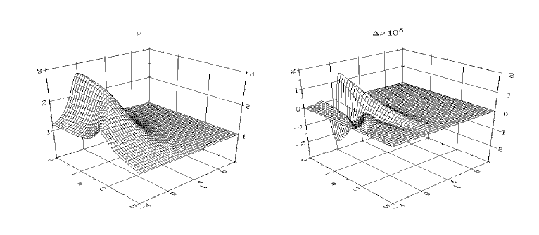
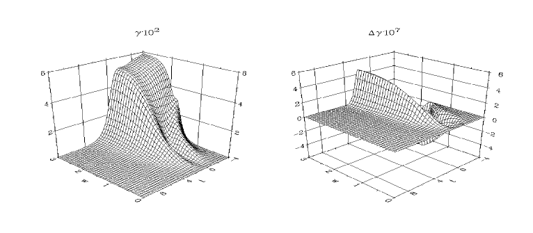
Figure 12: The numerical solutions for $\nu$ and $\gamma$ of the Weber-Wheeler wave for $a=0.5$, $b=2$ obtained with 1200 grid points in each region (left panels). In the right panels the corresponding deviation from the analytic result is amplified by $10^{5}$ and $10^{6}$, respectively. For presentation purposes $\nu$ and $\gamma$ are viewed from different angles.

We also see that longer runs do not reveal any new features as the metric variables approach their Minkowskian values after $t\approx 5$. This solution, however, does not provide a test for the rotational degree of freedom. For that purpose we need an analytic solution with both gravitational degrees of freedom.

3.5.2 Xanthopoulos’ rotating solution

The next solution we consider is one due to Xanthopoulos1986 which has a conical singularity on the $z$-axis and therefore describes a rotating vacuum solution with a cosmic string type singularity. The solution has been rewritten in terms of our variables by Sjodin2000. Again it is convenient to introduce auxiliary quantities

$$Q =r^{2}-t^{2}+1,$$ (3.55)

$$X =\sqrt{Q^{2}+4t^{2}},$$ (3.56)

$$Y =\frac{1}{2}[(2a^{2}+1)X+Q]+1-a\sqrt{2(X-Q)},$$ (3.57)

$$Z =\frac{1}{2}[(2a^{2}+1)X+Q]-1,$$ (3.58)

where $a$ is a free parameter which can take on any non-zero value. The solution derived by Xanthopoulos then becomes

$$\nu(t,\rho) =\frac{Z}{Y},$$ (3.59)

$$\tau(t,\rho) =-\frac{\sqrt{2(a^{2}+1)}\sqrt{X+Q}}{Y},$$ (3.60)

$$\gamma(t,\rho) =\frac{1}{2}\ln\frac{Z}{a^{2}X}.$$ (3.61)

In the outer region where we use the coordinates $(u,y)$ the result is

$$\tilde{Q} =y^{2}-u^{2}y^{2}-2u,$$ (3.62)

$$\tilde{X} =\sqrt{\tilde{Q}^{2}+4(uy^{2}+1)^{2}},$$ (3.63)

$$\tilde{Y} =\frac{1}{2}[(2a^{2}+1)\tilde{X}+\tilde{Q}]+y^{2}-ay\sqrt{2(\tilde{X}-\tilde{Q})},$$ (3.64)

$$\tilde{Z} =\frac{1}{2}[(2a^{2}+1)\tilde{X}+\tilde{Q}]-y^{2},$$ (3.65)

$$\nu(u,y) =\frac{\tilde{Z}}{\tilde{Y}},$$ (3.66)

$$\tau(u,y) =-\frac{\sqrt{2(a^{2}+1)}\sqrt{\tilde{X}+\tilde{Q}}}{\tilde{Y}},$$ (3.67)

$$\gamma(u,y) =\frac{1}{2}\ln\frac{\tilde{Z}}{a^{2}\tilde{X}}.$$ (3.68)

In Fig. 13 we show the numerical results and the deviation from the

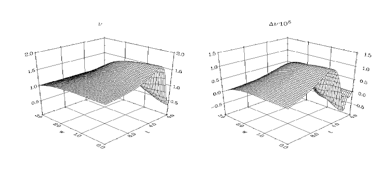
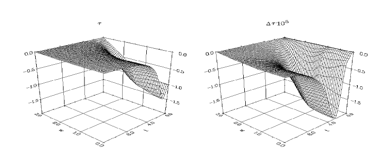
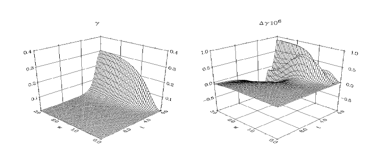
Figure 13: The numerical solutions for $\nu$, $\tau$ and $\gamma$ of Xanthopoulos’ spacetime for $a=1$ obtained with 300 grid points in each region (left panels). In the right panels the corresponding deviation from the analytic result is amplified by $10^{5}$ and $10^{6}$, respectively. The spatial coordinate $w$ is defined in Eq. (3.54).

analytic values obtained for $a=1$ and a Courant factor of 0.45. In this solution no steep gradients are present and 300 grid points in each region are sufficient to reproduce the analytic values to within a relative error of about $10^{-5}$. Again longer runs do not reveal any further features as the metric settles down into Minkowskian values. We conclude that the code reproduces analytic solutions with one or two gravitational degrees of freedom with high accuracy over the dynamically relevant time intervals.

3.5.3 Time dependent convergence analysis

Even though the accuracy and long term stability of the code has been demonstrated in the previous sections, we still have to make sure that it is also second order convergent. In particular the start-up procedure described in section 3.3.3 and the use therein of the Euler scheme to calculate the auxiliary time slice at $-dt/2$ might raise questions in this respect.
For the convergence analysis we define the $\ell_{2}$-norm of the deviation of a numerical solution $\Psi^{K}$ as a function of time

$$\Delta\Psi^{K}_{k} =\Psi^{K}_{k}-\Psi(x_{k}),$$ (3.69)

$$\ell_{2}[\Delta\Psi^{K}](t) =\sqrt{\frac{\sum_{k}{\left[\Delta\Psi^{K}_{k}(t)\right]^{2}}}{K}}.$$ (3.70)

Here $\Psi_{k}$ is the exact and $\Psi^{K}_{k}$ the numerical value at

Figure 14: The convergence factor $\ell_{2}[\Psi^{300}]/\ell_{2}[\Psi^{600}]$ is plotted as a function of time for the variables $\nu$, $\tau$ and $\gamma$. For our second order scheme we obtain a constant convergence factor of 4 expected for doubling the grid resolution.

grid point $k$ obtained for a total of $K$ grid points. We have calculated the $\ell_{2}$ norm for the Xanthopoulos solution of the previous section using 300 and 600 grid points in each region. In Fig. 14 we plot the quotient as a function of time. Corresponding to the increase of the grid resolution by a factor of 2 we expect a convergence factor of 4 for the second order scheme. In spite of the use of the first order Euler method for the start-up, second order convergence is clearly maintained throughout the dynamically relevant evolution.

4 Numerical evolution of excited cosmic strings

4.1 Introduction

According to the standard “big bang” model of cosmology, the universe is continuously expanding and cooling and was extremely hot and dense in its early stages. The grand unified theories (GUT) of elementary particle physics predict phase transitions to occur as a result of this cooling process in the early universe. These result in topological defects, regions with the “old symmetry” surrounded by “new symmetry”. The topology of the defects depends on the symmetry groups characterising the involved fields before and after the symmetry breaking. Cosmic strings are a 1-dimensional, “string-like” version of these topological defects. The type of strings usually considered from the astrophysical point of view has a mass per unit length $\mu\approx 10^{-6}$ in natural units ($\hbar=G=c=1$). The corresponding phase transitions are predicted to have occurred at the GUT energy scale $10^{15}$ GeV. Strings with significantly higher mass created at higher energy scales cannot be ruled out, however, and their treatment can no longer be achieved in the weak-field limit.
Numerical simulations by Vachaspati1984 show that cosmic strings are created in the form of a network of infinitely long or loop like strings. In this work we will focus on infinitely long strings which are modelled in the framework of cylindrical symmetry.
Cosmic strings have caught the interest of astrophysicists and relativists for several reasons. Most importantly the suggestion that cosmic strings be seeds for galaxy formation by Zeldovich1980 has given rise to intense efforts to understand the evolution of the resulting density perturbations (see e.g. Turok1986). Cosmic strings are also thought to be sources of gravitational radiation (Vilenkin1994). Below we will study the interaction of an infinitely long cosmic string with a wave pulse with one gravitational degree of freedom. Cosmic strings have also been considered of astrophysical relevance because of the bending of light rays that arises from the conical structure of the resulting spacetime. It has been shown by Vilenkin1981 that the geometry around an isolated cosmic string is Minkowskian minus a wedge, the “deficit angle”, and consequently cosmic strings may act as gravitational lenses.
Even though static cosmic strings in cylindrical symmetry have been studied extensively in the past either in Minkowskian or curved spacetime (see e.g. Laguna1987, Garfinkle1985), no solution has been obtained, to our knowledge, for a dynamic cosmic string coupled to gravity via the fully non-linear Einstein equations. Below we will present a numerical solution of this scenario and investigate the behaviour of a cosmic string excited by gravitational radiation. After presenting the mathematical description of a cosmic string in the next section we will derive the equations of a dynamic cosmic string coupled to gravity. In section 4.4 we will describe the numerical treatment of these equations. The simple scenario of a static cosmic string in Minkowski spacetime presents already most of the subtleties involved in solving the general problem and is therefore suitable for illustrating our numerical methods. Subsequently we address a static string in curved spacetime and finally present the dynamic code. This code is extensively tested in section 4.5 before we investigate the time evolution in section 4.6.
The results and techniques presented in this section can also be found in Sperhake2000.
We conclude this introduction with some comments on the numerical formulations used in this section. We have seen above how the combination of an interior Cauchy evolution with a characteristic evolution in the exterior region leads to a stable accurate simulation of cylindrically symmetry vacuum spacetimes. In a natural extension of this project we studied the inclusion of matter in the form of a cylindrically symmetric cosmic string. Such an extension of the CCM-code of the previous section has been developed, but no long term stable evolutions have been achieved with that code. Consequently we have restarted the investigation. For convenience this has been done in a purely characteristic framework and finally resulted in the long-term stable, accurate code described below. In the course of this work we have isolated the existence of exponentially diverging solutions and the corresponding difficulties at the outer boundary as the source of the problems. We will describe how these difficulties can be naturally controlled with the use of implicit numerical techniques. The use of such techniques, however, is by no means restricted to characteristic methods and we have no reason to believe that an implicit Cauchy-characteristic matching code would perform less satisfactorily. Such an implicit CCM code has been tested in the simple case of a cylindrically symmetric vacuum spacetime with vanishing rotation and has lead to an accurate long-term stable evolution of the Weber-Wheeler wave. From this point of view the choice of a characteristic formulation for the work described in this section is merely a consequence of the chronology in which progress has been achieved.

4.2 Mathematical description of a cosmic string

In the following work we will use cylindrical coordinates $r$, $\phi$, $z$. Here $z$ is the Killing direction corresponding to cylindrical symmetry and $r$, $\phi$ are standard polar coordinates. In 4-dimensional spacetime the time coordinate is $t$, but we will apply a characteristic formalism for the numerical solution and therefore also use the retarded time $u=t-r$. The simplest model of a cosmic string consists of a scalar field $\Phi$ coupled to a $U(1)$-gauge field $\hbox{\vec A}_{\mu}$. The Lagrangian for these coupled fields is given by

$$L_{M} =-|(\nabla_{\mu}+ie\hbox{\vec A}_{\mu})\Phi|^{2}-V(\Phi)-\frac{1}{4}\hbox{\vec F}_{\mu\nu}\hbox{\vec F}^{\mu\nu}.$$ (4.1)

Here $e$ is a constant, which describes the coupling between the scalar and the vector field. The self-coupling potential $V(\Phi)$ has the “Mexican-hat” shape predicted by the standard model of elementary particle physics and $\hbox{\vec F}_{\mu\nu}$ is the field tensor

$$\hbox{\vec F}_{\mu\nu} =\nabla_{\mu}\hbox{\vec A}_{\nu}-\nabla_{\nu}\hbox{\vec A}_{\mu},$$ (4.2)

$$V(\Phi) =2\lambda(\Phi^{2}-\langle\Phi\rangle^{2})^{2},$$ (4.3)

where $\lambda$ is the self-coupling constant of the scalar field. It turns out to be useful to introduce the Higgs vacuum expectation value of the scalar field as a parameter $\eta=2\langle\Phi\rangle^{2}$. Generalizing the notation of Garfinkle1985 we write the fields as

$$\Phi =\frac{S}{\sqrt{2}}e^{i\psi},$$ (4.4)

$$\hbox{\vec A}_{\mu} =\frac{1}{e}(P-1)\nabla_{\mu}\phi,$$ (4.5)

where $P$, $S$ and $\psi$ are functions of $u$, $r$, $\phi$. From now on, however, we will make the simplifying assumption of cylindrical symmetry. Then $P$ and $S$ are functions of $u$, $r$ only and $\psi=n\phi$, where $n$ is the winding number. In this work we will only consider the case $n=1$, so $\psi=\phi$. We can calculate the energy momentum tensor $\hbox{\vec T}^{\mu\nu}$ from the Lagrangian according to

$$\hbox{\vec T}^{\mu\nu} =\frac{2}{\sqrt{-\hbox{\vec g}}}\frac{\delta\mathcal{L}_{M}}{\delta\hbox{\vec g}_{\mu\nu}},$$ (4.6)

where $\mathcal{L}_{M}=\sqrt{-\hbox{\vec g}}L_{M}$ is the Lagrange density. Summarising the variables and parameters, we have

• the amplitude of the scalar field $S(u,r)$,

• the amplitude of the $U(1)$ gauge field $P(u,r)$,

• the constant $e$ which describes the coupling between the scalar and vector field,

• the self-coupling constant $\lambda$ of the scalar field,

• the vacuum expectation value of the scalar field $\eta$.

If we substitute Eqs. (4.4), (4.5) in (4.1) we obtain the Lagrangian and the energy momentum tensor in terms of these quantities

$$L_{M} =-\frac{1}{2}\hbox{\vec g}^{\mu\nu}(\nabla_{\mu}S)(\nabla_{\nu}S)-\frac{1}{2}S^{2}\hbox{\vec g}^{\mu\nu}(\nabla_{\mu}\phi+e\hbox{\vec A}_{\mu})(\nabla_{\nu}\phi+e\hbox{\vec A}_{\nu})-\lambda(S^{2}-\eta^{2})^{2}-\frac{1}{4}\hbox{\vec F}_{\mu\nu}\hbox{\vec F}^{\mu\nu},$$ (4.7)

$$\hbox{\vec T}_{\mu\nu} =(\nabla_{\mu}S)(\nabla_{\nu}S)+S^{2}(\nabla_{\mu}\phi+e\hbox{\vec A}_{\mu})(\nabla_{\nu}\phi+e\hbox{\vec A}_{\nu})+\hbox{\vec g}_{\mu\nu}L_{M}.$$ (4.8)

4.3 The field equations

We start again with the line element in Jordan, Ehlers, Kundt and Kompaneets (JEKK) form (3.10) for a cylindrically symmetric spacetime. This form of the metric, however, is not compatible with the cosmic string energy momentum tensor so we follow Marder1958 by introducing an extra variable $\mu$ into the metric

$$ds^{2}=e^{2(\gamma-\psi)}(-d\tilde{t}^{2}+d\tilde{r}^{2})+\tilde{r}^{2}e^{-2\psi}d\phi^{2}+e^{2(\psi+\mu)}(\omega d\phi+dz)^{2},$$ (4.9)

where the tilde is used to reserve the names $t$ and $r$ for rescaled coordinates below. This choice enables us to compare our numerical solutions with the results of the Cauchy-characteristic matching code described in section 3. We have already noted that this metric has a zero shift vector and the lapse is determined by the requirement $\hbox{\vec g}_{\tilde{t}\tilde{t}}=\hbox{\vec g}_{\tilde{r}\tilde{r}}$. The function $\mu$, however, introduces the extra gauge freedom of relabelling the radial null surfaces: $\tilde{u}\rightarrow f(\tilde{u})$ and $\tilde{v}\rightarrow g(\tilde{v})$. We may fix this by specifying the initial values for $\mu$ and either its time derivative in a “3+1” formalism or its boundary conditions in a characteristic formalism. We will follow the second approach and below we will see that the function $\mu$ is uniquely determined in the static case and the boundary conditions follow from regularity assumptions of the metric. The further requirement that the dynamic results reduce to the static ones in the case of vanishing time dependence therefore fixes the gauge.
It turns out that we can eliminate one of the free parameters and simplify the equations if we introduce rescaled quantities according to

$$t =\sqrt{\lambda}\eta\tilde{t},$$ (4.10)

$$r =\sqrt{\lambda}\eta\tilde{r},$$ (4.11)

$$X =\frac{S}{\eta},$$ (4.12)

$$\alpha =\frac{e^{2}}{\lambda}.$$ (4.13)

Thus $\alpha$ represents the relative strength of the coupling between scalar and vector field compared to the self-coupling. Furthermore we use the retarded time $u=t-r$ so that the line element becomes

$$ds^{2} =\frac{e^{2(\gamma-\psi)}}{\lambda\eta^{2}}(-du^{2}-2dudr)+r^{2}\frac{e^{-2\psi}}{\lambda\eta^{2}}d\phi^{2}+e^{2(\psi+\mu)}(\omega d\phi+dz)^{2}.$$ (4.14)

In section 3.3.1 we have described the Geroch decomposition which can be used to factor out the Killing direction $\mathchoice{{\hbox{\boldmath$\displaystyle\partial$}}}{{\hbox{\boldmath$\textstyle\partial$}}}{{\hbox{\boldmath$\scriptstyle\partial$}}}{{\hbox{\boldmath$\scriptscriptstyle\partial$}}}_{z}$ even if the Killing field is not hypersurface-orthogonal. It is a remarkable fact that the right hand side of equation (3.4) still vanishes for spacetimes with a cosmic string energy-momentum tensor (4.8) (Sjodin2000), so that the Geroch twist can be described by a potential according to Eq. (3.5). The other geometrical variable, the norm of the $z$-Killing vector (3.1) becomes

$$\nu=e^{2(\psi+\mu)},$$ (4.15)

and the 3-dimensional line element (3.3) is

$$ds^{2} =\frac{1}{\lambda\eta^{2}\nu}\left[e^{2(\gamma-\psi)}(-du^{2}-2dudr)+r^{2}e^{2\mu}d\phi^{2}\right].$$ (4.16)

With the energy momentum tensor given by (4.8) and the 3-dimensional line element (4.16) we are now in a position to calculate the field equations according to equations (3.6)-(3.8). We obtain

$$\begin{split}\Box\nu=&\,\,\nu_{,r}\mu_{,r}+\frac{\tau_{,r}^{2}-\nu_{,r}^{2}}{\nu}-\nu_{,u}\mu_{,r}-\nu_{,r}\mu_{,u}+2\frac{\nu_{,u}\nu_{,r}-\tau_{,u}\tau_{,r}}{\nu}\\[10.0pt] &+8\pi\eta^{2}\left[2e^{2(\gamma+\mu)}(X^{2}-1)^{2}+e^{-2\mu}\nu^{2}\frac{2P_{,u}P_{,r}-P_{,r}^{2}}{\alpha r^{2}}\right],\end{split}$$ (4.17)

$$\Box\tau= \,\,\tau_{,r}\mu_{,r}-2\frac{\tau_{,r}\nu_{,r}}{\nu}-\tau_{,u}\mu_{,r}-\tau_{,r}\mu_{,u}+2\frac{\tau_{,r}\nu_{,u}+\tau_{,u}\nu_{,r}}{\nu},$$ (4.18)

$$\Box\mu= \,\,\mu_{,r}^{2}+\frac{\mu_{,r}}{r}-\frac{\mu_{,u}}{r}-2\mu_{,u}\mu_{,r}+8\pi\eta^{2}\left[2\frac{e^{2(\gamma+\mu)}}{\nu}(X^{2}-1)^{2}+e^{2\gamma}\frac{X^{2}P^{2}}{r^{2}}\right]$$ (4.19)

$$0= \,\,2\gamma_{,r}+2r\gamma_{,r}\mu_{,r}-r\mu_{,rr}+r\mu_{,r}^{2}-\frac{r}{2\nu^{2}}(\tau_{,r}^{2}+\nu_{,r}^{2})-8\pi\eta^{2}\left[rX_{,r}^{2}+\frac{1}{\alpha}e^{-2\mu}\nu\frac{P_{,r}^{2}}{r}\right],$$ (4.20)

where we have introduced the flat-space d’Alembert operator

$$\Box=2\frac{\partial^{2}}{\partial u\partial r}-\frac{\partial^{2}}{\partial r^{2}}-\frac{1}{r}\left(\frac{\partial}{\partial r}-\frac{\partial}{\partial u}\right).$$ (4.21)

This set of equations is supplemented by the matter evolution equations obtained either from conservation of energy-momentum $\nabla_{\mu}\hbox{\vec T}^{\mu\nu}=0$ or variation of the Lagrange density $\mathcal{L}_{M}$ with respect to the matter fields $P$ and $X$. The result is

$$\Box P =2\frac{P_{,u}-P_{,r}}{r}-P_{,r}\mu_{,r}+P_{,r}\frac{\nu_{,r}}{\nu}+P_{,r}\mu_{,u}+P_{,u}\mu_{,r}-\frac{P_{,r}\nu_{,u}+P_{,u}\nu_{,r}}{\nu}-\alpha\frac{e^{2(\gamma+\mu)}}{\nu}PX^{2},$$ (4.22)

$$\Box X =X_{,r}\mu_{,r}-X_{,u}\mu_{,r}-X_{,r}\mu_{,u}-4\nu^{-1}e^{2(\gamma+\mu)}X(X^{2}-1)-e^{2\gamma}\frac{XP^{2}}{r^{2}}.$$ (4.23)

Note that in equations (4.17)-(4.20) the matter terms exclusively appear with a factor $\eta^{2}$. Consequently $\eta$ describes the effect of the string on the spacetime geometry and, thus, represents the string’s mass. There are two further Einstein equations which can be shown to be a direct consequence of (4.17)-(4.23) and their derivatives. These equations have only been used to provide a check on the accuracy of the code. Finally we have to supplement the equations by boundary conditions on the axis. For the 4-dimensional metric variables the simplest condition is to require the metric to be $C^{2}$ on the axis so that we have a well defined curvature tensor. The resulting boundary conditions are (Sjodin2001b)

$$\nu(t,r) =a_{1}(t)+\mathscr{O}(r^{2}),$$ (4.24)

$$\tau(t,r) =\mathscr{O}(r^{2}),$$ (4.25)

$$\mu(t,r) =a_{2}(t)+\mathscr{O}(r^{2}),$$ (4.26)

$$\gamma(t,r) =\mathscr{O}(r).$$ (4.27)

The boundary conditions for $S$ and $P$ are (Garfinkle1985)

$$P(t,r) =1+\mathscr{O}(r^{2}),$$ (4.28)

$$X(t,r) =\mathscr{O}(r).$$ (4.29)

The numerical implementation of these boundary conditions as well as regularity requirements at null infinity will be discussed in section 4.4.3.

4.4 Numerical methods

In order to solve the above field equations we have developed two independent codes. The first is based on the Cauchy characteristic matching code described in section 3. This code performs well in the absence of matter and has been used to study several cylindrically symmetric vacuum solutions (see also Sjodin2000). However, this CCM code performed less satisfactorily in the evolution of the cosmic string. This is due to the existence of unphysical solutions to the evolution equations (4.17)-(4.23) which diverge exponentially as $r\rightarrow\infty$. Controlling the time evolution near null infinity by means of a sponge function enabled us to select the physical solutions with regular behaviour at $I^{+}$, but the sponge function itself introduced noise which eventually gave rise to instabilities. We therefore implemented a second implicit, purely characteristic, code which allows us to directly control the behaviour of the solutions at the boundaries and thus suppress diverging solutions. The main problem with the system of differential equations is the irregularity of the equations at both the origin and null infinity. It is the implicit nature of the scheme that provides a simple way of implementing the boundary conditions and thus circumventing all problems with these irregularities. A purely characteristic formulation has been used for the second code for convenience rather than numerical necessity and we believe that an implicit CCM scheme would produce similar accuracy, convergence and long term stability. It is interesting that the irregularity problems are already present in the calculation of the static cosmic string in Minkowski spacetime. We will, therefore, first describe the numerical scheme used in the static Minkowskian case where the equations are fairly simple. We then present the modifications necessary for the static and dynamic case coupled to the gravitational field.

4.4.1 The static cosmic string in Minkowski spacetime

In Eqs. (4.17)-(4.23) we set the metric variables to their Minkowskian values and all time derivatives to zero to obtain the equations for the static cosmic string in Minkowski spacetime (cf. Garfinkle1985)

$$r\frac{d}{dr}\left(r^{-1}\frac{dP}{dr}\right) =\alpha X^{2}P,$$ (4.30)

$$r\frac{d}{dr}\left(r\frac{dX}{dr}\right) =X\left[P^{2}+4r^{2}(X^{2}-1)\right].$$ (4.31)

The boundary conditions are (see Garfinkle1985)

$$P(0) =1, \lim_{r\rightarrow\infty}P(r) =0,$$

$$X(0) =0, \lim_{r\rightarrow\infty}X(r) =1.$$ (4.32)

In order to cover the whole spacetime with a finite coordinate range, we divide the computational domain into two regions in the same way as in section 3.3.3. In the inner region ($0\leq r\leq 1$) we use the coordinate $r$, while in the outer region we introduce the compactified radius $y$ defined by equation (3.12) which covers the range $1\geq y\geq 0$. This corresponds to the region $1\leq r<\infty$ with infinity mapped to $y=0$. Again we combine $r$ and $y$ into the single radial variable $w$ defined by (3.54). In terms of the coordinate $y$ Eqs. (4.30), (4.31) take the form

$$\frac{d}{dy}\left(y^{5}\frac{dP}{dy}\right)=4\alpha\frac{X^{2}P}{y},$$ (4.33)

$$\frac{d}{dy}\left(y\frac{dX}{dy}\right)=4X\left[\frac{P^{2}}{y}+4\frac{(X^{2}-1)}{y^{5}}\right].$$ (4.34)

The number of grid points in each region may differ, but

Figure 15: The combined grid of the inner and the outer region. Note that both grid points, $K_{1}$ and $K_{1}+1$, correspond to the position $r=1\Leftrightarrow y=1$. These points form the interface of the code and facilitate transformation of the variables from the coordinate system using $r$ into that using $y$.

each half-grid is uniform. Thus we use a total of $K:=K_{1}+K_{2}$ grid points where the points labelled $K_{1}$ and $K_{1}+1$ both correspond to the position $r=1=y$. The points $K_{1}$, $K_{1}+1$ form the interface between the two regions (see Fig. 15). One point will contain the variables in terms of $r$, the other in terms of $y$. With the computational grid covering the whole spacetime, we now face a two point boundary value problem. Due to the existence of unphysical solutions diverging at $y=0$ we have chosen to solve the equations with a numerical relaxation scheme as described in section 2.3.5 which allows us to directly control the behaviour of $P$ and $X$ at infinity. The form of Eqs. (4.30), (4.31) suggests that in order to write them as a first order system we should introduce the auxiliary variables $Q=r^{-1}P_{,r}$ and $R=rX_{,r}$. The equations may then be written in the form

$$P_{,r} =rQ,$$ (4.35)

$$X_{,r} =\frac{R}{r},$$ (4.36)

$$Q_{,r} =\alpha\frac{PX^{2}}{r},$$ (4.37)

$$R_{,r} =X\left[\frac{P^{2}}{r}+4r(X^{2}-1)\right].$$ (4.38)

The corresponding equations in the outer region are given by

$$P_{,y} =-2\frac{Q}{y^{5}},$$ (4.39)

$$X_{,y} =-2\frac{R}{y},$$ (4.40)

$$Q_{,y} =-2\alpha\frac{X^{2}P}{y},$$ (4.41)

$$R_{,y} =-2X\left(\frac{P^{2}}{y}+4\frac{X^{2}-1}{y^{5}}\right).$$ (4.42)

Standard second order centred finite differencing according to Eqs. (2.78), (2.79) results in $4(K-2)$ non-linear algebraic equations which are supplemented by the 4 boundary conditions (4.32) and 4 interface relations

$$P_{K_{1}+1} =P_{K_{1}},$$ (4.43)

$$X_{K_{1}+1} =X_{K_{1}},$$ (4.44)

$$Q_{K_{1}+1} =Q_{K_{1}},$$ (4.45)

$$R_{K_{1}+1} =R_{K_{1}}.$$ (4.46)

We then start with piecewise linear initial guesses for $P$ and $X$ (and the corresponding derivatives $Q$ and $R$) and solve the $4K$ algebraic equations as described in section 2.3.5.
In order to check the code for convergence, we vary the grid resolution $K$ (using $K_{1}=K_{2}$ points in both regions) from $150$ to $2400$, halving the grid spacing each time. Since we do not have an analytic solution, the results are compared against the high-resolution case ($K=2400$). For doing this we calculate the $\ell_{2}$ norm according to Eq. (3.70). In this case the function $\Psi$ in Eq. (3.70) stands for $P$, $X$, $Q$ or $R$ and the norm does not depend on time because of the static nature of the problem. For second order convergence we expect the $\ell_{2}$ norm to decrease by a factor of 4 each time we increase the grid resolution by a factor of 2. However, we do not compare our results against the exact solution but against a high resolution result which itself has a finite truncation error, so that

$$\ell_{2}[\Psi^{K}] =\left(\sum_{k}\Psi^{K}_{k}-\Psi^{2400}_{k}\right)^{1/2}.$$ (4.47)

Therefore we do not expect the factor to be exactly $4$. Using a

Table 1: Convergence test for the cosmic string in Minkowski space-time for $\alpha=1$. The norm of the deviation $\ell_{2}[\Delta\Psi^{K}]$ is defined by Eq. (4.47). As the grid resolution is increased, the deviation from the high resolution result decreases quadratically to a good approximation (see text for details).

	P	X	Q	R
$\ell_{2}(\Delta\Psi^{1200})$	$5.77\cdot 10^{-7}$	$2.84\cdot 10^{-7}$	$5.86\cdot 10^{-7}$	$8.89\cdot 10^{-7}$
$\ell_{2}(\Delta\Psi^{150})/\ell_{2}(\Delta\Psi^{300})$	4.05	4.05	4.04	4.05
$\ell_{2}(\Delta\Psi^{300})/\ell_{2}(\Delta\Psi^{600})$	4.20	4.20	4.20	4.20
$\ell_{2}(\Delta\Psi^{600})/\ell_{2}(\Delta\Psi^{1200})$	5.00	5.00	5.00	5.00

grid resolution $K$ the truncation error is given by

$$\Psi^{K} =\Psi+\mathscr{O}\left(\frac{1}{K^{2}}\right),$$ (4.48)

where $\Psi$ is the exact and $\Psi^{K}$ the numerical solution. For simplicity we will assume that the truncation error is either $-1/K^{2}$ or $+1/K^{2}$. If we use a reference solution obtained for $4K$ grid points and compare solutions $\Psi^{K}$ and $\Psi^{2K}$ the ratio of the corresponding $\ell_{2}$-norms becomes

$$\left(\frac{\sum(\Psi_{i}^{K}-\Psi_{i}^{4K})^{2}}{\sum(\Psi_{i}^{2K}-\Psi_{i}^{4K})^{2}}\right)^{1/2} =\left(\frac{\sum(\pm\frac{1}{K^{2}}\pm\frac{1}{16K^{2}})^{2}}{\sum(\pm\frac{1}{4K^{2}}\pm\frac{1}{16K^{2}})^{2}}\right)^{1/2}=\left|\frac{\pm 16\pm 1}{\pm 4\pm 1}\right|.$$ (4.49)

Considering the extreme cases, we expect a convergence factor between 3 and $5\frac{2}{3}$. The truncation error of the high resolution result will have significantly less influence on the comparison of lower resolution results and the factors should be closer to 4. Table 1 shows our results for the cosmic string in Minkowski space-time and clearly indicates second order convergence. In Fig. 16 we show the string variables $P$ and $X$ for various values of $\alpha$ as a function of $w$.

Figure 16: The cosmic string variables $P$ and $X$ are plotted for $\alpha=$ 10, 1, 0.1, 0.01 (from “left to right”). The two families are labelled in the plot. As $\alpha$ increases, both, $P$ and $X$ become more concentrated towards the origin. Note that $w=3$ corresponds to $r\to\infty$ [cf. Eq. (3.54)].

Due to the rescaling (4.10)-(4.12) the equations for the cosmic string in Minkowski spacetime (4.30) and (4.31) do not explicitly contain the parameter $\eta$, so the shape of the cosmic string fields expressed in terms of the rescaled variables is independent of $\eta$. Below we will see that this is no longer true in curved spacetime where $\eta$, representing the mass of the string, determines the strength of its coupling to gravity. Fig. 16 does, however, reveal a significant variation of the profiles of the scalar and vector field with the coupling ratio $\alpha$. As the scalar-vector coupling becomes more dominant with respect to the self coupling of the scalar field (larger $\alpha$), both $P$ and $X$ become more concentrated towards the origin.

4.4.2 The static cosmic string coupled to gravity

The equations governing a static cosmic string in curved spacetime are obtained from the general equations (4.17)-(4.23) by setting all time derivatives to zero. If we combine first and second spatial derivatives in a single operator as in equations (4.30), (4.31), we can write these equations as

$$(r\nu_{,r})_{,r}= \,\,-r\nu_{,r}\mu_{,r}+r\frac{\nu_{,r}^{2}-\tau_{,r}^{2}}{\nu}+8\pi\eta^{2}\left[e^{-2\mu}\nu^{2}\frac{P_{,r}^{2}}{\alpha r}-2e^{2(\gamma+\mu)}r(X^{2}-1)^{2}\right],$$ (4.50)

$$(r\tau_{,r})_{,r}= \,\,2r\frac{\tau_{,r}\nu_{,r}}{\nu}-r\tau_{,r}\mu_{,r}\ ,$$ (4.51)

$$(r^{2}\mu_{,r})_{,r}= \,\,-r^{2}\mu_{,r}^{2}-8\pi\eta^{2}\left[e^{2\gamma}X^{2}P^{2}+2e^{2(\gamma+\mu)}\nu^{-1}r^{2}(X^{2}-1)^{2}\right],$$ (4.52)

$$\gamma_{,r}= \,\,\frac{r}{2(r\mu_{,r}+1)}\left[\mu_{,rr}-\mu_{,r}^{2}+\frac{1}{2\nu^{2}}\left(\tau_{,r}^{2}+\nu_{,r}^{2}\right)+8\pi\eta^{2}\left(X_{,r}^{2}+\frac{1}{\alpha}e^{-2\mu}\nu\frac{P_{,r}^{2}}{r^{2}}\right)\right],$$ (4.53)

$$\left(\frac{1}{r}P_{,r}\right)_{,r}= \,\,\frac{P_{,r}\mu_{,r}}{r}-\frac{P_{,r}\nu_{,r}}{r\nu}+\alpha e^{2(\gamma+\mu)}\nu^{-1}\frac{PX^{2}}{r},$$ (4.54)

$$(rX_{,r})_{,r}= \,\,-rX_{,r}\mu_{,r}+X\left[e^{2\gamma}\frac{P^{2}}{r}+4e^{2(\gamma+\mu)}\nu^{-1}r(X^{2}-1)\right].$$ (4.55)

After completing the code, we realised that in the case of vanishing rotation $\tau$ the field equations (4.50)-(4.55) imply a simple relation between $\nu$, $\mu$ and $\gamma$. An appropriate linear combination of these equations and their spatial derivatives can be written as

$$(\gamma+\mu-\ln{\nu})_{,rr}+\left(\frac{1}{r}+\mu_{,r}\right)(\gamma+\mu-\ln{\nu})_{,r} =0,$$ (4.56)

which after some manipulation becomes

$$(\gamma+\mu-\ln{\nu})_{,r} =C\frac{e^{-\mu}}{r}.$$ (4.57)

Here $C$ is a constant that has to vanish in order to ensure finite derivatives at the origin. In the static case we adjust the functions $a_{1}$ and $a_{2}$ in the boundary conditions (4.24), (4.26) so that $\nu=1$ and $\mu=0$ at the origin and consequently

$$\gamma+\mu-\ln{\nu} =0,$$ (4.58)

for all values of $r$. Even though $\tau$ will be zero in the analysis in this section, we will numerically solve the original system of equations (4.50)-(4.55) and use (4.58) as a test for the code.
In order to numerically solve the equations of a cosmic string coupled to gravity, we rewrite them again as a first order system. The differential operators appearing on the right hand side suggest that we introduce the auxiliary quantities $N=r\nu_{,r}$, $T=r\tau_{,r}$, $M=r^{2}\mu_{,r}$, $Q=r^{-1}P_{,r}$ and $R=rX_{,r}$. The system can then be written in the form

$$\nu_{,r} =\frac{N}{r},$$ (4.59)

$$\tau_{,r} =\frac{T}{r},$$ (4.60)

$$\mu_{,r} =\frac{M}{r^{2}},$$ (4.61)

$$P_{,r} =rQ,$$ (4.62)

$$X_{,r} =\frac{R}{r},$$ (4.63)

$$N_{,r} =\frac{N^{2}-T^{2}}{r\nu}-\frac{NM}{r^{2}}-16\pi\eta^{2}e^{2\gamma+2\mu}r(X^{2}-1)^{2}+8\pi\frac{\eta^{2}}{\alpha}e^{-2\mu}\nu^{2}rQ^{2},$$ (4.64)

$$T_{,r} =2\frac{TN}{\nu r}-\frac{TM}{r^{2}},$$ (4.65)

$$M_{,r} =-\frac{M^{2}}{r^{2}}-8\pi\eta^{2}e^{2\gamma}X^{2}P^{2}-16\pi\eta^{2}e^{2\gamma+2\mu}\nu^{-1}r^{2}(X^{2}-1)^{2},$$ (4.66)

$$2(r+M)\gamma_{,r} =M_{,r}-2\frac{M}{r}-\frac{M^{2}}{r^{2}}+\frac{T^{2}+N^{2}}{2\nu^{2}}+8\pi\eta^{2}R^{2}+8\pi\frac{\eta^{2}}{\alpha}e^{-2\mu}\nu r^{2}Q^{2},$$ (4.67)

$$Q_{,r} =\frac{QM}{r^{2}}-\frac{QN}{r\nu}+\alpha e^{2\gamma+2\mu}\nu^{-1}\frac{PX^{2}}{r},$$ (4.68)

$$R_{,r} =-\frac{RM}{r^{2}}+4e^{2\gamma+2\mu}\nu^{-1}rX(X^{2}-1)+e^{2\gamma}\frac{XP^{2}}{r}.$$ (4.69)

The corresponding equations in terms of the compactified radial coordinate $y$ are

$$\nu_{,y} =\frac{N}{y},$$ (4.70)

$$\tau_{,y} =\frac{T}{y},$$ (4.71)

$$\mu_{,y} =yM,$$ (4.72)

$$P_{,y} =\frac{Q}{y^{5}},$$ (4.73)

$$X_{,y} =\frac{R}{y},$$ (4.74)

$$N_{,y} =\frac{N^{2}-T^{2}}{y\nu}-yNM-64\pi\eta^{2}e^{2\gamma+2\mu}\frac{(X^{2}-1)^{2}}{y^{5}}+8\pi\frac{\eta^{2}}{\alpha}e^{-2\mu}\nu^{2}\frac{Q^{2}}{y^{5}},$$ (4.75)

$$T_{,y} =2\frac{TN}{y\nu}-yTM,$$ (4.76)

$$M_{,y} =-yM^{2}-32\pi\eta^{2}e^{2\gamma}\frac{X^{2}P^{2}}{y^{3}}-64\pi\eta^{2}e^{2\gamma+2\mu}\nu^{-1}\frac{(X^{2}-1)^{2}}{y^{7}},$$ (4.77)

$$2(y^{2}M-2)\gamma_{,y}= \,\,\,y^{2}M_{,y}+4yM-y^{3}M^{2}+\frac{N^{2}+T^{2}}{2y\nu^{2}}+8\pi\eta^{2}\frac{R^{2}}{y}+8\pi\frac{\eta^{2}}{\alpha}e^{-2\mu}\nu\frac{Q^{2}}{y^{5}},$$ (4.78)

$$Q_{,y} =yQM-\frac{QN}{y\nu}+4\alpha e^{2\gamma+2\mu}\nu^{-1}\frac{PX^{2}}{y},$$ (4.79)

$$R_{,y} =-yRM+4e^{2\gamma}\frac{XP^{2}}{y}+16e^{2\gamma+2\mu}\nu^{-1}\frac{X(X^{2}-1)}{y^{5}}.$$ (4.80)

From the numerical point of view, the problem of solving these equations is virtually identical to that of a static string in Minkowski spacetime. The only difference is the much higher degree of complexity of the equations due to the appearance of $\nu$, $\tau$, $\mu$ and $\gamma$ as extra variables. We will discuss the numerical implementation of the boundary conditions at the origin and at infinity in the next section when we consider the case of a dynamic cosmic string. The boundary conditions are given by equations (4.104), (4.105). In the static case we replace the conditions for $N$, $T$ and $M$ in (4.104) by

$$\begin{split}\nu=1,\\[5.0pt] \tau=0,\\[5.0pt] \mu=0,\end{split}$$ (4.81)

but otherwise use the same boundary conditions. The solution is then obtained using the relaxation method described in the previous section. As our initial guess for the metric variables we use Minkowskian values, and for the string variables $X$ and $P$ we use the previously calculated values for a Minkowskian string with the same string parameters. Due to the appearance of $\tau$ or its derivatives in all terms of (4.51) the Geroch potential will

Table 2: Convergence test for the static cosmic string in curved space-time for $\alpha=1$. The norm of the deviation $\ell_{2}[\Delta\Psi^{K}]$ is defined by Eq. (4.47). As the grid resolution is increased, the deviation from the high resolution result decreases quadratically to a good approximation (see text for details).

	$\nu$	$\mu$	$\gamma$	P $X$
$\ell_{2}(\Delta\Psi^{1200})$	$1.28\cdot 10^{-7}$	$2.51\cdot 10^{-6}$	$2.39\cdot 10^{-6}$	$5.95\cdot 10^{-7}$	$4.16\cdot 10^{-7}$
$\ell_{2}(\Delta\Psi^{150})/\ell_{2}(\Delta\Psi^{300})$	3.56	3.59	3.58	4.04	3.37
$\ell_{2}(\Delta\Psi^{300})/\ell_{2}(\Delta\Psi^{600})$	3.76	3.79	3.78	4.19	3.60
$\ell_{2}(\Delta\Psi^{600})/\ell_{2}(\Delta\Psi^{1200})$	4.58	4.61	4.60	4.98	4.44

stay zero in the relaxation process and our solution has no rotation.
We have checked the code for convergence in the way described in section 4.4.1. We have chosen the unphysically large value $\eta=0.2$ here in order to guarantee convergence even for strong coupling between matter and geometry. $\alpha$ is set to 1 as in the Minkowski case. The results are given in Table 2. For convenience we only display the results for the fundamental variables $\nu$, $\mu$, $\gamma$, $P$ and $X$. Since we do not incorporate rotation, the result for $\tau$ is, as expected, exactly 0 and we do not include it in Table 2. Again the code is shown to be second order convergent.

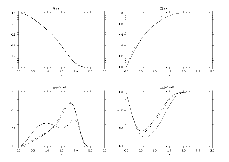
Figure 17: a) In the upper two panels we plot the string variables for $\eta=$ 0.001 (dotted) and 0.2 (solid) as a function of the radial variable $w$. b) In the lower panels we have plotted the deviation from the Minkowskian values rescaled by $\eta^{2}$ for $\eta=$ 0.001 (dotted), 0.01 (dashed), 0.1 (long dashed) and 0.2 (solid). Note that the curves for 0.001 and 0.01 almost exactly coincide, which indicates the validity of the linear regime. For larger $\eta$, however, the deviation shows a more complicated behaviour.

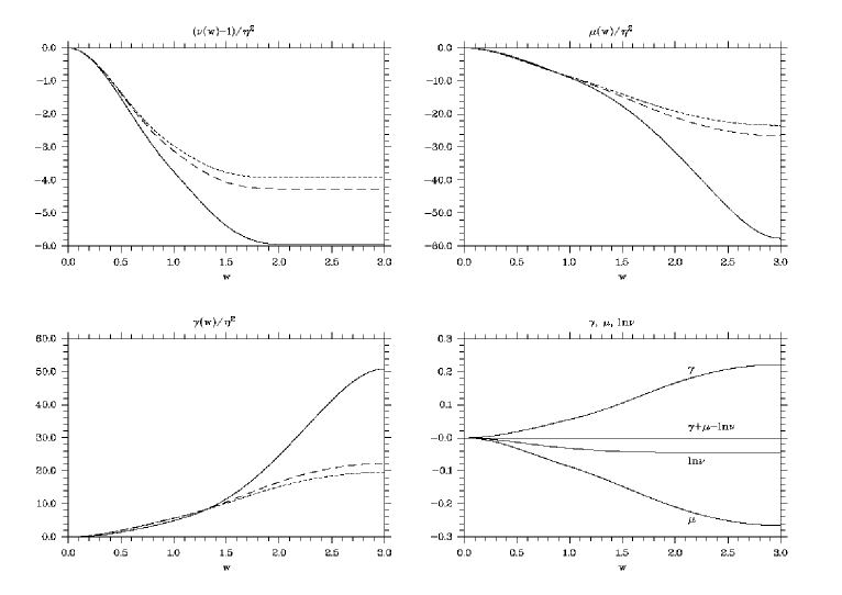
Figure 18: The deviation of the metric variables $\nu$, $\mu$ and $\gamma$ from Minkowskian values rescaled by $\eta^{2}$ is plotted as a function of $w$ for $\eta=$ 0.001 (dotted), 0.01 (dashed), 0.1 (long dashed) and 0.2 (solid). The dotted and the dashed curves almost exactly coincide indicating the linear regime. As in the case of the string variables we find a more complicated dependence for $\eta\geq 0.1$. In the lower right panel we plot $\gamma$ $\mu$, $\ln{\nu}$ and their sum for $\eta=0.1$ which vanishes in accordance with Eq. (4.58) to high accuracy.

In Fig. 17 and 18 we plot the results obtained for $N=2400$ grid points. In all these plots the relative coupling strength is $\alpha=1$, but qualitatively similar results are obtained for different values of $\alpha$. We have already mentioned that the effect of the string on the spacetime geometry is determined by $\eta$. Therefore we have compared the deviation of both the string variables and the metric from the Minkowskian case for $\eta=$ 0.001, 0.01, 0.1 and 0.2. In Fig. 17 we plot the string variables $P$ and $X$ for the two extreme values and the deviation from the Minkowskian string rescaled by $\eta^{2}$ for all four values. For small $\eta$ we see that $\Delta P/\eta^{2}$ and $\Delta X/\eta^{2}$ is essentially independent of $\eta$. In this case the deviation from Minkowskian values can be treated as a small perturbation and a linear dependence of $\Delta P$ and $\Delta X$ on $\eta^{2}$ is to be expected. In the range $\eta=0.1\ldots 0.2$ on the other hand, we clearly leave the linear regime and the deviation depends on $\eta$ in a much more complicated way. These values, however, are 2 orders of magnitude larger than the value $10^{-3}$ predicted in current GUT theories (Vilenkin1994). The deviation of the metric variables $\nu$, $\mu$ and $\gamma$ is plotted in the first three panels of Fig. 18. Again we see the linear behaviour for small $\eta$ and the transition to the non-linear regime at $\eta\approx 0.1$. In the fourth panel of Fig. 18 we check Eq. (4.58) for $\eta=0.1$. We clearly see that $\gamma+\mu+\ln{\nu}$ is approximately zero. Indeed (4.58) is satisfied to within $\approx 10^{-8}$ as compared with the order of magnitude of the individual terms $10^{-1}$.

4.4.3 The dynamic cosmic string

In the dynamic case all variables $\nu$, $\tau$, $\mu$, $\gamma$, $P$ and $X$ are functions of $u,r$ and we have to solve the system (4.17)-(4.23) of partial differential equations. In order to control the behaviour of the solution at infinity, we need a generalisation for PDEs of the relaxation scheme applied to ordinary differential equations. In view of the characteristic feature of the relaxation scheme, namely the simultaneous calculation of new function values at all grid points, this generalisation leads directly to implicit evolution schemes as used for hyperbolic or parabolic PDEs. Therefore, the dynamic code is based on the implicit, second order in space and time Crank-Nicholson scheme described in section 2.3.6. For this purpose we rewrite the dynamic equations (4.17)-(4.23) as a first order system. These equations involve radial derivatives which may be written in terms of second order operators exactly as in the static case (4.50)-(4.55). This naturally leads to the auxiliary quantities introduced in Eqs. (4.59)-(4.63). In terms of these variables the equations for the dynamic cosmic string become

$$\nu_{,r}= \frac{N}{r},$$ (4.82)

$$\tau_{,r}= \frac{T}{r},$$ (4.83)

$$\mu_{,r}= \frac{M}{r^{2}},$$ (4.84)

$$P_{,r}= rQ,$$ (4.85)

$$X_{,r}= \frac{R}{r},$$ (4.86)

$$\begin{split}2N_{,u}=&N_{,r}+\frac{T^{2}-N^{2}}{r\nu}+\frac{NM}{r^{2}}+2\frac{\nu_{,u}N-\tau_{,u}T}{\nu}-\nu_{,u}-\frac{\nu_{,u}M}{r}-N\mu_{,u}\\[10.0pt] &+8\pi\eta^{2}\left[2e^{2(\gamma+\mu)}r(X^{2}-1)^{2}+\frac{1}{\alpha}e^{-2\mu}\nu^{2}(2P_{,u}Q-rQ^{2})\right],\end{split}$$ (4.87)

$$2T_{,u}= T_{,r}-2\frac{TN}{r\nu}+2\frac{\tau_{,u}N+\nu_{,u}T}{\nu}+\frac{TM}{r^{2}}-\tau_{,u}-\frac{\tau_{,u}M}{r}-T\mu_{,u},$$ (4.88)

$$2M_{,u}= M_{,r}+\frac{M^{2}}{r^{2}}-2\mu_{,u}M-2r\mu_{,u}+8\pi\eta^{2}\left[e^{2\gamma}X^{2}P^{2}+2\frac{e^{2(\gamma+\mu)}}{\nu}r^{2}(X^{2}-1)^{2}\right],$$ (4.89)

$$2(r+M)\gamma_{,r}= M_{,r}-2\frac{M}{r}-\frac{M^{2}}{r^{2}}+\frac{T^{2}+N^{2}}{2\nu^{2}}+8\pi\eta^{2}\left[R^{2}+\frac{1}{\alpha}e^{-2\mu}\nu r^{2}Q^{2}\right],$$ (4.90)

$$2Q_{,u}= Q_{,r}-\frac{QM}{r^{2}}+Q\mu_{,u}-\frac{Q\nu_{,u}}{\nu}-\frac{P_{,u}N}{r^{2}\nu}+\frac{QN}{r\nu}+\frac{P_{,u}}{r^{2}}+\frac{P_{,u}M}{r^{3}}-\alpha\frac{e^{2(\gamma+\mu)}}{\nu}\frac{PX^{2}}{r},$$ (4.91)

$$2R_{,u}= R_{,r}-X_{,u}-\frac{X_{,u}M}{r}+\frac{RM}{r^{2}}-R\mu_{,u}-4\frac{e^{2(\gamma+\mu)}}{\nu}rX(X^{2}-1)-e^{2\gamma}\frac{XP^{2}}{r}.$$ (4.92)

The corresponding first order system in the outer region is given by

$$\nu_{,y}= -2\frac{N}{y},$$ (4.93)

$$\tau_{,y}= -2\frac{T}{y},$$ (4.94)

$$\mu_{,y}= -2yM,$$ (4.95)

$$P_{,y}= -2\frac{Q}{y^{5}},$$ (4.96)

$$X_{,y}= -2\frac{R}{y},$$ (4.97)

$$\begin{split}2N_{,u}=&-\frac{1}{2}y^{3}\left(N_{,y}-2yNM-2\frac{T^{2}-N^{2}}{y\nu}\right)-y^{2}\nu_{,u}M+2\frac{\nu_{,u}N-\tau_{,u}T}{\nu}\\[10.0pt] &-N\mu_{,u}-\nu_{,u}+8\pi\eta^{2}\left[2e^{2(\gamma+\mu)}\frac{(X^{2}-1)^{2}}{y^{2}}+\frac{1}{\alpha}e^{-2\mu}\nu^{2}\left(2P_{,u}Q-\frac{Q^{2}}{y^{2}}\right)\right],\end{split}$$ (4.98)

$$2T_{,u}= -\frac{1}{2}y^{3}\left(T_{,y}-2yTM+4\frac{TN}{y\nu}\right)-T\mu_{,u}-y^{2}\tau_{,u}M+2\frac{\tau_{,u}N+\nu_{,u}T}{\nu}-\tau_{,u},$$ (4.99)

$$\begin{split}2M_{,u}=&-\frac{1}{2}y^{3}(M_{,y}-2yM^{2})-2\frac{\mu_{,u}}{y^{2}}-2\mu_{,u}M\\[10.0pt] &+8\pi\eta^{2}\left[e^{2\gamma}X^{2}P^{2}+2\frac{e^{2(\gamma+\mu)}}{\nu}\frac{(X^{2}-1)^{2}}{y^{4}}\right],\end{split}$$ (4.100)

$$2(y^{2}M+1)\gamma_{,y}= \,\,\,y^{2}M_{,y}+4yM+2y^{3}M^{2}-\frac{N^{2}+T^{2}}{y\nu^{2}}-16\pi\eta^{2}\left[\frac{R^{2}}{y}+\frac{1}{\alpha}e^{-2\mu}\nu\frac{Q^{2}}{y^{5}}\right],$$ (4.101)

$$\begin{split}2Q_{,u}=&-\frac{1}{2}y^{3}\left(Q_{,y}+2yQM-2\frac{QN}{y\nu}\right)+y^{4}P_{,u}-y^{4}\frac{P_{,u}N}{\nu}-\frac{\nu_{,u}Q}{\nu}\\[10.0pt] &+y^{6}P_{,u}M+Q\mu_{,u}-\alpha e^{2(\gamma+\mu)}\nu^{-1}y^{2}PX^{2},\end{split}$$ (4.102)

$$\begin{split}2R_{,u}=&-\frac{1}{2}y^{3}(R_{,y}-2yRM)-X_{,u}-R\mu_{,u}-y^{2}X_{,u}M-e^{2\gamma}y^{2}XP^{2}\\[10.0pt] &-4e^{2(\gamma+\mu)}\nu^{-1}\frac{X(X^{2}-1)}{y^{2}}.\end{split}$$ (4.103)

The derivation of these equations and a number of other calculations in this work have been carried out with the algebraic computing package GRTensorII (Musgrave1996). In order to solve these equations we must supplement them by appropriate initial and boundary conditions. We have already mentioned the boundary conditions on the axis (4.24)-(4.29). In general we find that the dynamic code performs better if one imposes boundary conditions on the radial derivatives rather than the variables themselves. For the variables $\nu$, $\mu$, $\tau$, $P$ and $X$ we therefore impose the required boundary conditions on the initial data according to (4.32) and (4.81). In the subsequent evolution we impose the weaker condition that the radial derivatives $N$, $T$ and $R$ are finite on the axis. This ensures that the evolution equations propagate the axial conditions given on the initial data. For the variable $\mu$ we impose the condition that $M$ is zero on the axis which is equivalent to the rather weak condition that $r^{2}\mu_{r}$ vanishes there. The inverse power of $r$ in the definition of $Q$ makes it unsuitable to specify the value of this quantity at $r=0$ so in this case we work with the variable directly and require that $P=1$ on the axis. Finally the variable $\gamma$ is given by a purely radial equation and in this case we specify the value on the axis where $\gamma$ vanishes by virtue of Eq. (4.27). Therefore at $r=0$ we require

$$\begin{split}N&=0,\\ T&=0,\\ M&=0,\\ \gamma&=0,\\ P&=1,\\ R&=0.\end{split}$$ (4.104)

For the boundary conditions at null infinity we know that regular solutions of the cylindrical wave equation have radial derivatives that decay faster than $1/r$ so that we may take the variables $N$, $T$, and $R$, which satisfy a wave type equation, to vanish at $y=0$. The asymptotics of $\mu$ are slightly different due to the additional power of $r$ in the radial derivative (similar to the spherically symmetric wave equation) but for a regular solution $\mu_{,y}$ vanishes at null infinity. The equation for $P$ does not satisfy a wave type equation due to the inverse power of $r$ but has asymptotic behaviour given by a modified Bessel function. The physically relevant finite solution has exponential decay so in this case one may impose the condition that $Q=0$ at $y=0$. Hence we require the solution to satisfy the following boundary conditions at $y=0$

$$\begin{split}N&=0,\\ T&=0,\\ \mu_{,y}&=0,\\ Q&=0,\\ R&=0.\end{split}$$ (4.105)

These boundary conditions are sufficient to determine the solution of the first order system (4.82)-(4.103) while suppressing the unphysical solutions which are singular on the axis or null infinity. Note that $\gamma$ is determined by the constraint equation (4.20), which is a first order ODE, and thus only needs one boundary condition.
We finally note that all variables are related at the interface in the form $f_{K_{1}+1}=f_{K}$ analogous to Eqs. (4.43)-(4.46) in the case of a static string in Minkowski spacetime.

4.5 Testing the dynamic code

In this section we will describe four independent tests of the implicit code for the dynamic cosmic string, namely

• reproducing the non-rotating vacuum solution of Weber1957,

• reproducing the rotating vacuum solution of Xanthopoulos1986,

• using the results for the static cosmic string as initial data and verifying that the system stays in its static configuration,

• convergence analysis for the string hit by a Weber-Wheeler wave.

Two additional tests arise in a natural way from the field equations and the numerical scheme. As described above there are two additional field equations which are consequences of the other equations. We have verified that these equations are satisfied to second order accuracy ($\sim\Delta r^{2}$). Furthermore the numerical scheme calculates the residuals of the algebraic equations to be solved, which have thus been monitored in test runs. They are satisfied to a much higher accuracy (double precision machine accuracy), so the total error is dominated by the truncation error of the second order differencing scheme. Another independent test is the comparison with the explicit CCM code which yields good agreement as long as the latter remains stable. The four main tests are now described in more detail.

4.5.1 The Weber-Wheeler wave

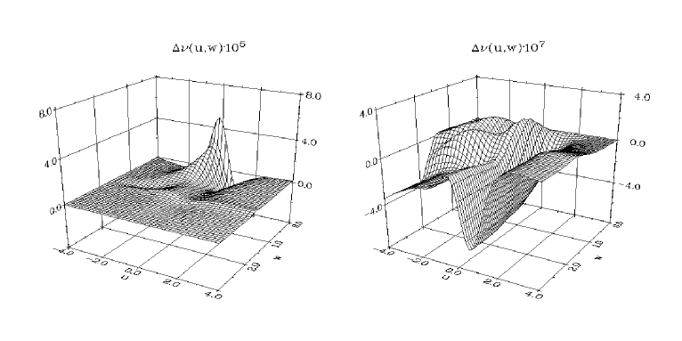
Figure 19: The deviation of the numerical $\nu$ and $\gamma$ from the Weber-Wheeler solution as a function of $u$ and $w$ obtained for 1920 grid points ($K_{1}=320$, $K_{2}=1600$). The wave parameters are $a=2$, $b=0.5$. Note that the error is amplified by $10^{5}$ and $10^{7}$ respectively.

In the first test we evolve the analytic solution given by Weber1957, which describes a gravitational pulse of the “+” polarisation mode. We have given the analytic expressions in section 3.5.1 in terms of $t$, $r$ [Eqs. (3.46)-(3.49)] and in terms of $u$, $y$ [Eqs. (3.50)-(3.53)]. The corresponding equations in characteristic coordinates $u$, $r$ in the inner region are easily obtained from the coordinate transformation $t=u+r$. We prescribe $\nu$ as initial data according to the analytic expressions obtained for $a=2$ and $b=0.5$ and set the other free variables to zero, while $\gamma$ is calculated via quadrature from the constraint equation (4.20). In Fig. 19 we show the deviation of the numerical results from the analytic one for $K=1920$ grid points (320 points in the inner, 1600 points in the outer region) and a Courant factor of 0.5 with respect to the inner region. The convergence analysis (see below) shows that this number of points provides sufficient resolution in the outer region while still keeping computation times at a tolerable level. All computations presented in the remainder of section 4 have been obtained with these grid parameters, unless stated otherwise. The code stays stable for much longer time intervals than shown in the figure, but does not reveal any further interesting features as the analytic solution approaches its Minkowskian values and the error goes to zero.

4.5.2 The rotating solution of Xanthopoulos

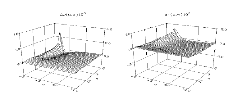
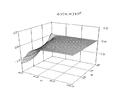
Figure 20: The deviation of the numerical $\nu$, $\tau$, $\gamma$ from Xanthopoulos’ analytic solution as a function of $u$ and $w$ obtained for 1920 grid points ($K_{1}=320$, $K_{2}=1600$). Note that the error is amplified by $10^{5}$ and $10^{6}$ respectively.

Xanthopoulos1986 has derived an analytic vacuum solution for Einstein’s field equations in cylindrical symmetry containing both the “+” and “$\times$” polarisation mode. Its analytic form in terms of our metric variables is given by Eqs. (3.55)-(3.68) in section 3.5.2. Again the transformation to coordinates $u$, $r$ in the inner region results straightforwardly from $t=u+r$. The solution has one free parameter $a$ set to one in this calculation. The error of our numerical results is displayed in Fig. 20, where we have used the same grid parameters as in the Weber-Wheeler case. Again we have run the code for longer times and found that the error approaches zero. We conclude that the code reproduces both analytic vacuum solutions with excellent accuracy comparable to that of the CCM code and exhibits long term stability.

4.5.3 Evolution of the static cosmic string

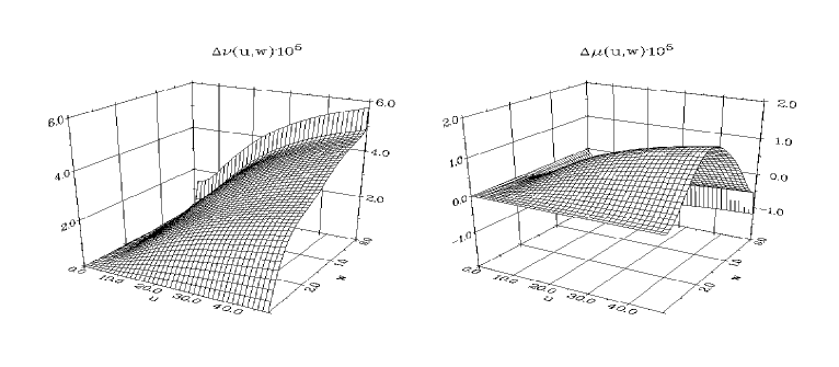
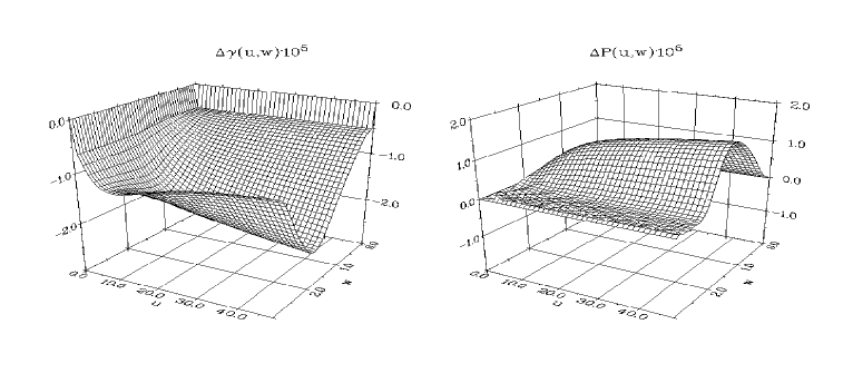
Figure 21: The deviation of the metric and matter variables from the initial data in the case of evolving a static cosmic string with $\alpha=1$, $\eta=0.2$. For our standard grid with $1920$ points, the configuration stays static to an accuracy of $\approx 10^{-5}$ over a range of more than 30000 time steps.

The tests described above only involve vacuum solutions, so the matter part of the code and the interaction between matter and geometry has not been tested. An obvious test involving matter and geometry is to use the result for the static cosmic string in curved spacetime as initial data and evolve this scenario. All variables should, of course, remain at their initial values. We have evolved the static string data for our standard grid and the parameter set, $\alpha=1$ and $\eta=0.2$, which corresponds to a strong back-reaction of the string on the metric. The results are shown in Fig. 21. The system stays in its static configuration with high accuracy over a time interval which is significantly longer than the dynamically relevant timescale of the vacuum solutions discussed above.

4.5.4 Convergence analysis

Figure 22: The convergence factor $\ell_{2}[\Psi^{1920}]/\ell_{2}[\Psi^{2880}]$ is plotted as a function of $u$. We expect a convergence factor of 2.25 since the number of grid points is multiplied by 1.5. Even though our results show weak variability at later times, second order convergence is maintained throughout long runs (more than 30000 time steps with $K=1920$).

Our investigation of the interaction between the cosmic string and gravitational waves will focus on the string being hit by a wave of the Weber-Wheeler type. In order to check this scenario for convergence we have run the code for the parameter set $\eta=0.2$, $\alpha=1$, $a=2$, $b=0.5$ for different grid resolutions, where $a$ and $b$ are again the width and amplitude of the Weber-Wheeler wave. In our case it is of particular interest to investigate the time dependence of the convergence to see what resolution we need in order to obtain reliable results for long runs. We calculate the convergence rate again according to equation (3.70). The high resolution reference solution has been calculated for $K=4320$ grid points. In Fig. 22 we show the convergence factor $\ell_{2}[\Psi^{1920}]/\ell_{2}[\Psi^{2880}]$ as a function of $u$ for $\nu$, $\mu$, $\gamma$, $P$ and $X$. The initial data for $\tau$ is identically zero for this scenario and stays zero during the evolution. The number of grid points is increased by a factor of 1.5 here (instead of the more commonly used 2) to reduce the computation time. Only points common to all grids have been used in the sum in equation (3.70). For second order convergence we would expect a convergence factor of $1.5^{2}$. Although the results in Fig. 22 show weak variations with $u$, second order convergence is clearly maintained for long runs. In each case the outer region contains 5 times as many grid points as the inner region (e.g. $K_{1}=320$, $K_{2}=1600$ for the $K=1920$ case). The reason for this is that in the dynamic evolutions $X$ and especially $P$ exhibit significant spatial variations out to large radii. Due to the compactification, the spatial resolution of our grid decreases towards null infinity and in order to resolve the spatial variations of the string variables out to sufficiently large radii we therefore have to introduce a large number of grid points in the outer region. No such problems occur in the inner region. If significantly fewer grid points are used in the outer region for this analysis, the convergence properties of the string variables can deteriorate to roughly first order level.

4.6 Time dependence of the string variables

4.6.1 Static cosmic strings excited by gravitational waves

Figure 23: The initial data for $\nu$, $P$ and $X$ at $u_{0}=-20$ for the standard parameters $\alpha=1$, $\eta=0.001$, $a=2$, $b=0.5$. The gravitational wave pulse is located in a region where the string fields $P$ and $X$ have almost fallen off to their asymptotic values.

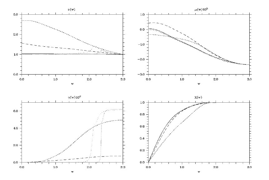
Figure 24: The metric and string variables are plotted as functions of $w$ at $u=-20$ (dotted), $u=-10$ (long dotted), $u=0$ (dashed), $u=2$ (long dashed) and $u=10$ (solid line). For clarity the graphs of $P$ are distributed over two panels. The wave pulse (in $\nu$) initially moves inwards. It excites the string, is reflected at the origin and travels outwards. After $u=10$ only $P$ differs significantly from the static configuration as the oscillations slowly decay and propagate towards larger radii (cf. Fig. 25).

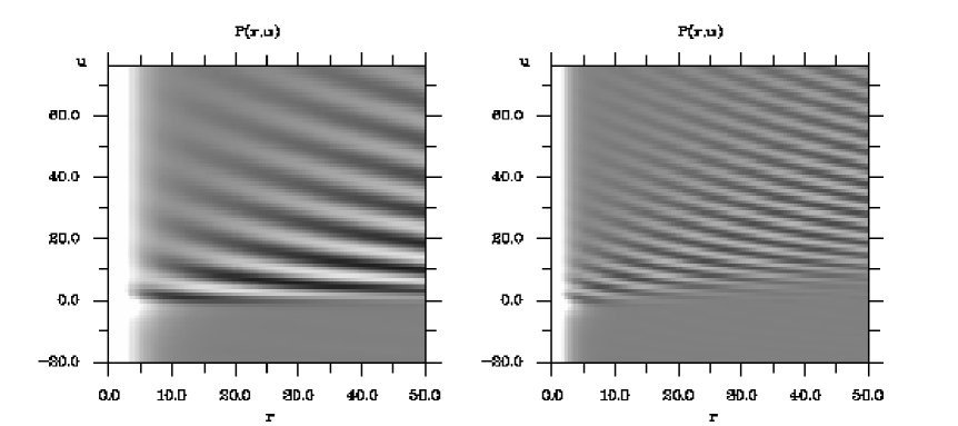
Figure 25: The cosmic string variable $P$ is shown as a function of radius and time for $\alpha=0.2$ (left) and $\alpha=1$ (right) (all other parameters have standard values). Note that we use the radial variable $r$ out to $r=50$ here. The ringing can clearly be seen and shows a lower frequency for smaller $\alpha$.

The scenario we are going to investigate in this section is an initially static cosmic string hit by a gravitational wave of Weber-Wheeler type. For this purpose we use the static results with two modifications as initial data. Firstly the static metric function $\nu_{0}$ is multiplied by the exact Weber-Wheeler solution to simulate the gravitational wave pulse. Thus we guarantee that initially the cosmic string is indeed in an equilibrium configuration provided the wave pulse is located sufficiently far away from the origin and its interaction with the string is negligible. Ideally the numerical calculation would start with the incoming wave located at past null infinity. In order to approximate this scenario, we found it was sufficient to use the large negative initial time $u_{0}=-20$. The second modification is to calculate $\gamma$ from the constraint equation (4.20) to preserve consistency with the Einstein field equations. In Fig. 23 the corresponding initial data for $\nu$, $P$ and $X$ are shown for the parameter set $\eta=0.001$, $\alpha=1$, $a=2$ and $b=0.5$. From now on we will refer to these values as “standard parameters” and only specify parameters if they take on non-standard values. The time evolution of the “standard configuration” is shown in Fig. 24 where we plot $\nu$, $\mu$, $\gamma$, $P$ and $X$ as functions of $w$ at times $-20$, $-10$, $0$, $2$ and $10$. While the wave pulse is still far away from the origin, its interaction with the cosmic string is negligible (dotted lines). When it reaches the core region it excites the cosmic string and the scalar and vector field start oscillating (dashed curves). After being reflected at the origin, the wave pulse travels along the outgoing characteristics and the metric variables $\nu$, $\mu$ and $\gamma$ quickly settle down into their static configuration which is close to Minkowskian values for $\eta=10^{-3}$. The vector and scalar field of the cosmic string, on the other hand, continue ringing albeit with a different character. Whereas the oscillations of the scalar field $X$ are dominant in the range $r\leq 2$ and have significantly decayed at $u=10$ as shown in the figure, the vector field oscillations propagate to large radii and fall off very slowly (solid curves). This behaviour is also illustrated in the right panel of Fig. 25 which shows a contour plot of $P$ as a function of $(u,r)$ out to $r=50$. We shall see below, that the oscillations of $P$ will also decay eventually and the cosmic string will asymptotically settle back into its equilibrium configuration.

4.6.2 Frequency analysis

We will now quantitatively analyse the oscillations of the scalar and vector field of the cosmic string. Since we are working in rescaled coordinates, physical time and distance are measured in units of $1/\sqrt{\lambda}\eta$ and frequency in its inverse. To avoid complicated notation, however, we will omit the units from now on unless the meaning is unclear. In order to measure frequencies, we Fourier analyse the time evolution of the scalar and vector field for fixed radius $r$. Fig. 26 shows $P$ and $X$ for standard parameters as functions of time at $r=1$ together with the corresponding power spectra. In each Fourier spectrum we can see three peaks. Those very close to $f=0$ are merely due to the offset of the data and the gradual change of the fields over long times. We therefore do not attribute these peaks to the oscillations of the fields and will not consider them in the ensuing discussion. We have calculated similar power spectra for a large class of parameter sets and in most cases found two peaks at non-zero frequencies. In order to interprete the frequencies, it is convenient to plot them as functions of the relative coupling strength $\alpha$. The result is shown in Fig. 27. In this figure the solid lines show the frequency values calculated for the scalar and vector field from the linearised equations (see Sjodin2001)

$$f_{X} =\frac{\sqrt{2}}{\pi},$$ (4.106)

$$f_{P} =\frac{\sqrt{\alpha}}{2\pi}.$$ (4.107)

We can thus associate the constant frequency $f=0.45$ with the scalar field $X$ and the $\alpha$ dependent frequency with the vector field $P$. We will refer to these frequencies as $f_{X}$ and $f_{P}$ from now on. The $\alpha$-dependency of $f_{P}$ is also illustrated in Fig. 25 where we show contour plots of $P$ obtained for $\alpha=0.2$ and $\alpha=1$. The oscillation frequency is significantly larger for $\alpha=1$.
In Fig. 27 we can see that the frequencies associated with the scalar and vector field become similar near $\alpha=8$. For this value it can be shown that the masses associated with the scalar and vector field become equal (see for example Sjodin2001). The frequencies are difficult to resolve in these cases and we have only found one peak in the Fourier spectra. The resulting values are shown as filled lozenges in the figure. In this context it is worth mentioning that the accuracy of the measurements of the frequencies is limited by the resolution of the Fourier spectra which again is limited by the time interval covered in the evolution. In Fig. 26 we can see however, that the oscillations of both $P$ and $X$ gradually die out in later stages of the evolutions, so that it becomes increasingly difficult to extract more information about the frequencies by using larger integration times. The evolutions used for this analysis provide an accuracy $\Delta f\approx 0.01$ which corresponds approximately to one bin in the frequency spectra.
It is interesting to see that in the non-linear evolution the distinction between the oscillations of the vector and the scalar field is not as clear as in the linear case which is demonstrated by the presence of two peaks in the Fourier spectra. We attribute this feature to the interaction between the scalar and vector component of the cosmic string. Concerning the radial dependence of the spectra we have in general found that the characteristic mode of $X$ resulted in stronger peaks at smaller radius, that of $P$ was stronger at larger radii. This variation of the relative strength of the oscillations with radius confirms the corresponding observation in Fig. 24.

Figure 26: Upper panels: The variables $P$ and $X$ at $r=1$ are plotted as functions of $u$ for $\alpha=1$, $\eta=0.001$, $a=2$ and $b=0.5$. Lower panels: The corresponding power spectra show three peaks each. That near $f=0$ is merely due to a constant offset and the variation of the fields on long time scales and thus not associated with the oscillations. From the linear equations one can infer that the peaks at $f=0.45$ can be identified with the oscillation of the scalar field, the peaks at $f=0.16$ with those of the vector field. Note that due to our rescaling of the coordinates, $u$ is measured in units of $1/\sqrt{\lambda}\eta$.

In order to investigate the dependency of the oscillations on

Figure 27: The frequencies obtained from the Fourier analysis of the oscillations of the scalar and vector fields are plotted as functions of $\alpha$. The curves show the frequencies of the scalar and vector field predicted by an analysis of the linearised equations. For $5\leq\alpha\leq 8$ the predicted values for $P$ and $X$ are similar and we find only one frequency. These values are plotted as filled lozenges.

$\eta$, $a$, $b$ and the radial position $r$, we have varied each parameter over at least two orders of magnitude while keeping the other parameters at standard values. We have found the following dependencies:

• The frequencies of both $X$ and $P$ do not show any variations with $\eta$ for $\eta<0.1$. (Note that $\eta$ does, however, appear in the units). For larger values of $\eta$, the non-linear interaction between string and geometry becomes dominant and we did not detect a simple relation between frequency maxima and parameters.

• The variation of the parameters $a$ and $b$, the width and amplitude of the Weber-Wheeler pulse, has no measurable effect on the frequencies of $X$ and $P$, but only determined the amplitude of the oscillations. A narrow, strong pulse leads to larger amplitudes.

• For small $r$ the oscillations in $X$ are stronger, whereas those for $P$ dominate at large $r$. The frequency values, however, do not depend on the radius. For radii greater than 10 the oscillations in $X$ had decayed so strongly that we could no longer measure its frequency.

We have also checked the empirical relation between the coupling constant $\alpha$ and the frequencies $f_{X}$ and $f_{P}$. For this purpose we have performed a linear regression analysis of the double logarithmic data of Fig. 27 excluding the cases where only one frequency is observed. We obtain power law indices $\sigma_{X}=0.00$ and $\sigma_{P}=0.50$, so that

$$f_{X} \sim{\rm const},$$ (4.108)

$$f_{P} \sim\sqrt{\alpha},$$ (4.109)

which agrees with Eqs. (4.106), (4.107). If we transform this result back into physical units using $\alpha=e^{2}/\lambda$, we arrive at the following relations for the physical variables

$$f_{X} \sim\sqrt{\lambda}\eta,$$ (4.110)

$$f_{P} \sim e\eta.$$ (4.111)

As shown in Shellard1994 up to constant factors $\sqrt{\lambda}\eta$ and $e\eta$ are the masses of the scalar and the vector field, $m_{X}$ and $m_{P}$, so that $X$ and $P$ have characteristic frequencies

$$f_{X} \sim m_{X},$$ (4.112)

$$f_{P} \sim m_{P}.$$ (4.113)

Since the frequencies for $X$ and $P$ seem only to depend upon the respective masses we have attempted to confirm these results by considering the oscillations of a cosmic string in two further scenarios. Firstly since the frequencies do not depend upon the shape of the Weber-Wheeler

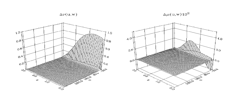
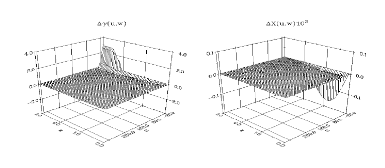
Figure 28: The upper four plots show the difference between the evolved functions $\nu$, $\mu$, $\gamma$ and $X$ and their corresponding static results. For $P$ a similar 3-dimensional plot is not suitable since it fails to resolve the oscillations of the vector field. Therefore we plot the $\ell_{2}$-norm (dashed line) and the maximum (solid line) of $\Delta P$ as a function of time. $\nu$, $\mu$, $\gamma$ and $X$ quickly settle down in their equilibrium configuration to numerical accuracy. The decay of the oscillations of $P$ takes significantly more time but eventually $P$ also approaches its equilibrium state.

pulse we take as initial data the static values for the metric variables but excite the string by adding a Gaussian perturbation to either the $X$ or $P$ static initial values. The evolution is then computed using the fully coupled system. Secondly since the frequencies do not seem to depend upon the strength of the coupling to the gravitational field we have completely decoupled the gravitational field and considered the evolution of a cosmic string in Minkowski spacetime. The initial data is taken to be that for a static string in Minkowski spacetime with a Gaussian perturbation to either the $X$ or $P$ values. The evolution is then computed using the equations for a dynamical string in a Minkowskian background [equations (4.22) and (4.23) with the metric variables set to Minkowskian values]. In both cases we obtain the same frequencies, to within an amount $\Delta f=0.01$, that we find in the original case of the fully coupled system excited by a Weber-Wheeler pulse. Furthermore the frequencies did not depend on the location or shape of the field perturbation nor upon the choice of $X$ or $P$ as the perturbed field.

4.6.3 The long term behaviour of the dynamic string

The time evolution shown in Figs. 24 and 25 indicates that the oscillations of the cosmic string excited by gravitational waves gradually decay and metric and string settle down into an equilibrium state. In order to investigate the long term behaviour in detail we have evolved the variables for a much longer time ($-20\leq u\leq 410$) than in the numerical evolutions discussed above. The unphysically large value of $\eta=0.1$ is chosen for this calculation in order to guarantee a strong interaction between spacetime geometry and the cosmic string. In Fig. 28 we show the difference $\Delta f:=f_{\rm evol}-f_{\rm stat}$ between the time-dependent $\nu$, $\mu$, $\gamma$ and $X$ and their corresponding static results obtained for the same parameters. For the vector field $P$ a similar 3-dimensional plot would require an extreme resolution to properly display the oscillations of the vector field (cf. Fig. 24). For this reason we proceed differently and calculate the $\ell_{2}$-norm and the maximum of $\Delta P$ for each slice $u={\rm const}$. Both functions are plotted versus time in Fig. 28. The incoming wave pulse can clearly be seen as a strong deviation of $\nu$ from the static function. The pulse excites the cosmic string and is reflected at the origin at $u=0$. The metric variables and the scalar field $X$ then quickly reach their equilibrium values. The oscillations in $P$ decay on a significantly longer time scale which is also evident in Figs. 24 and 25 and the $\ell_{2}$-norm of $\Delta P$ slowly approaches 0. Significantly longer runs than shown here are prohibited by the required computation time, but the results indicate that $P$ will also eventually reach its equilibrium configuration.

4.7 Discussion

In the previous two sections we have studied numerical problems in cylindrical symmetry with particular emphasis on the use of characteristic methods and the compactification of spacetime.
This work has completed the 1-dimensional stage of the Southampton Cauchy-characteristic matching project by presenting for the first time a long-term stable second order convergent code for general cylindrically symmetric vacuum spacetimes with both the $+$ and $\times$ polarisation mode. In order to obtain long-term stability it was crucial to formulate the problem in a way that simplifies the relations at the interface where information is transferred between the interior Cauchy and the exterior characteristic region. In this particular case we achieved the simplification by applying the Geroch decomposition to both regions which contrasts with the less successful previous attempts where the Killing direction was factored out in the exterior region only. In view of the numerical subtleties involved with the interpolation techniques at the interface the importance of a suitable choice of variables may not be too surprising. Nevertheless we stress the significance of this result concerning Cauchy-characteristic matching codes in higher dimensions. The structure of the null geodesics will inevitably become much more complicated if the restriction of cylindrical symmetry is dropped and the physical variables are allowed to depend on the angular coordinates. Correspondingly the transformation between variables at the interface will also be more complicated. In view of our results it seems important to carefully choose the variables describing the spacetime in both regions and aim for “simple” transformation laws.
The inclusion of matter in the form of cosmic strings resulted in qualitatively new numerical problems that finally were solved by the use of specially adapted numerical methods. The incorporation of null infinity proved to be important here for the specification of outer boundary conditions on the matter variables. It was the existence of unphysical exponentially diverging solutions of the equations for a cosmic string that required a special numerical treatment. We were able to suppress the unphysical diverging solutions by solving the equations for a cosmic string with a relaxation scheme in the static case and an implicit evolution scheme in the dynamic case. We have thus been able to develop the first fully non-linear simulation of a static and a dynamic cosmic string coupled to gravity which implements the exact boundary conditions at both the origin and infinity. The resulting codes have been used to study the interaction between a cosmic string and a gravitational wave pulse. We have found that the gravitational wave pulse excites the cosmic string which then starts oscillating with frequencies proportional to the particle masses associated with the scalar and vector field. The same frequencies have been observed if we excite the cosmic string with a Gaussian perturbation to the scalar or vector field.
From a numerical point of view an interesting result of the numerical solution of the equations for a dynamic cosmic string concerns the transfer of information at the interface. We have illustrated this in Fig. 15 where two grid points $K_{1}$, $K_{1}+1$ have been used for the spatial position $r=1$. The grid point $K_{1}$ contains the variables of the interior region at $r=1$, whereas the variables of the exterior region are specified at the same position on grid point $K_{1}+1$. The corresponding implementation of the interface is remarkably simple as illustrated by Eqs. (4.43)-(4.46) which represent the interface for the static cosmic string in Minkowski spacetime. The corresponding equations in the dynamic case coupled to gravity are equally trivial. Even if different variables are used in the interior and exterior region, one is still able to transform the variables locally at the grid points $K_{1}$ and $K_{1}+1$ and there is no need to use interpolation techniques as in the case of the explicit numerical methods used in section 3. We attribute the possibility of using this simple implementation of the interface to the fact that all function values are calculated simultaneously on the new time slice in an implicit scheme, so that there is no hierarchical order according to which the function values have to be calculated. We have probed such a “local interface” in an implicit Cauchy-characteristic matching code for cylindrically symmetric, non-rotating vacuum spacetimes and achieved a long term stable evolution with an accuracy comparable to the explicit code described in section 3. Even though an interface based on interpolation performs satisfactorily in cylindrical symmetry this may no longer be the case in higher dimensional problems where the interpolation techniques will be significantly more complicated. On the other hand we can see no obvious reason why a “local interface” in combination with an implicit numerical scheme should differ significantly from that used in the 1-dimensional case.

5 Non-linear oscillations of spherically symmetric stars

5.1 Introduction

In this section we will turn our attention towards the study of compact stars in the framework of general relativity. The discovery of stars significantly more compact than the sun goes back to observations of the binary star Sirius in the middle of the 19th century. Sirius is the brightest star in the sky as viewed from the earth. From an astrophysical point of view, however, the faint companion of the bright main star, Sirius B has provoked much more interest. The astronomer Bessel was the first to infer the existence of an unseen companion of Sirius from a wobble in the motion of the main star. It took another twenty years before Alvin Clark managed to optically resolve Sirius B. By the early twentieth century it became clear from the analysis of its electromagnetic spectrum that Sirius B has a rather high surface temperature of about 25,000$\,K$. In view of this result the extraordinarily low luminosity of Sirius B lead to the conclusion that the star is very small, about the size of the earth. This type of high density star was consequently named a white dwarf. It was understood at the time that white dwarfs mark the final stage in the evolution of stars, but it remained a puzzle how such compact objects were able to support themselves against gravitational contraction. The answer was first provided by Eddington and Fowler who suggested that the star is supported by the degenerate electron pressure, a quantum effect arising from the Pauli-exclusion principle. When Chandrasekhar worked out the corresponding theory for a relativistic electron gas he made the remarkable discovery that the degenerate electron pressure will never be sufficient to support white dwarfs above a mass of about $1.4\,M_{\odot}$. In his words: “For a star of small mass the natural white dwarf stage is an initial step towards complete extinction. A star of large mass cannot pass into the white dwarf stage and one is left speculating on other possibilities.” It did not take long before such speculations were directed towards the existence of neutron stars.
The first suggestion that stars made up of nucleons may exist came from Landau in 1932 just two years after the discovery of the neutron. Two years later Baade and Zwicky proposed the idea that neutron stars may be the product of supernova explosions and thus mark the final stage in the evolution of stars of large mass. The first theoretical models of neutron stars were calculated in 1939 by Tolman, Oppenheimer and Volkoff. It took another thirty years, however, before neutron stars were actually discovered observationally. Furthermore this discovery came in a completely unexpected way. In 1967 the then Cambridge graduate student Jocelyne Bell and her supervisor Antony Hewish were looking for scintillations of radio sources produced by the interstellar medium. On the 28th of November 1967 they discovered a source with an exceptionally regular pattern of radio pulses which at the time even gave rise to the speculation of an extra-terrestrial, intelligent origin. These speculations were quickly abandoned, however, when three more “pulsars” were found within the next few weeks. The extremely short duration of the pulses and the high pulse frequencies lead to the conclusion that these sources must be significantly smaller than white dwarfs. An explanation for this phenomenon was finally found when a pulsar was detected at the centre of the crab nebula. From historical records it is known that the crab nebula marks a supernova explosion that was observed in the year 1054. Pulsars are therefore identified with neutron stars, the remnants of supernova explosions. In the same way that the degeneracy pressure of the electrons supports white dwarfs against gravitational collapse, the internal pressure in neutron stars arises from the degenerate nucleons. A great deal of work has gone into the observational and theoretical study of these compact objects. From these studies it is known that neutron stars have masses of about $1.4$ solar masses and radii of about $10\,{\rm km}$. Neutron stars are believed to have a solid crust in which the density increases from about $10^{4}\,{\rm g/cm}^{3}$ to a few times $10^{11}\,{\rm g/cm}^{3}$. In this density range the matter is assumed to consist of a degenerate electron gas and atomic nuclei that form a crystal-like structure. At larger densities the atomic nuclei gradually dissolve and at about $2\cdot 10^{14}\,{\rm g/cm}^{3}$ the matter largely consists of a highly incompressible neutron fluid with small amounts of protons and electrons. An interesting property of this fluid arises from the thermal temperature which is commonly believed to be smaller than $10^{8}\,{\rm K}$. Compared with the Fermi-temperature of the nucleons of about $3\cdot 10^{11}\,{K}$ this implies that the matter behaves like a fluid at zero temperature and becomes superfluid and, in the case of the protons, super-conductive. The structure of matter and the resulting equations of state at higher densities become increasingly unclear and are subject to ongoing research. Near the centre of a neutron star the density is assumed to be of the order of $10^{15}\,{\rm g/cm}^{3}$ and the matter may at least partly consist of hyperons, pions or quarks, so-called strange matter.
The extreme compactness of neutron stars makes them particularly interesting from a relativistic point of view. We have already mentioned the significance of neutron stars in the context of the search for gravitational waves. In this respect the importance of neutron star oscillations arises from the discovery of secularly unstable oscillation modes that increase in amplitude due to the spin down of the neutron star while energy is radiated away in the form of gravitational waves. If the attempts to measure gravitational waves are indeed successful, a whole new window for astrophysical observations may be opened and facilitate a unique opportunity to directly observe the interior of astrophysical objects such as neutron stars. In this work, however, we will not directly study neutron star oscillations in the context of gravitational radiation. Instead we use the simpler case of spherically symmetric dynamic neutron stars in order to probe a new numerical approach which enables us to numerically evolve non-linear oscillations of arbitrary amplitude with high accuracy. While these evolutions will not lead to the generation of gravitational waves because of the spherical symmetry, the numerical results, the new techniques and the discussion of numerical difficulties encountered in the course of this work may still be relevant for numerical simulations of more general types of neutron star oscillations.
The use of oscillations as a diagnostic tool to obtain information about the interior structure of an object is an old idea and by no means restricted to the realm of distant stars. For example the same technique has been applied to the earth where the study of artificially induced oscillations and, in particular, earthquakes has lead to invaluable insight into the internal structure of our planet. In the same way a great deal of knowledge has been obtained about the sun and more distant stars by investigating their oscillations which reveal themselves in the electromagnetic spectra of these objects. Whereas Newtonian theory is perfectly adequate for studying “normal” stars, i.e. stars that gain their energy from continuous nuclear burning of hydrogen and other light elements, accurate modelling of compact objects like neutron stars requires a general relativistic description.
The first type of neutron star oscillations to be studied extensively were linear radial oscillations (see for example Chandrasekhar1964a, Chandrasekhar1964b) which today represent a well understood problem that is described in the standard literature. The same is not true, however, for nonlinear radial oscillations which lead to qualitatively new problems. We have already mentioned that spherically symmetric spacetimes do not admit radiative solutions. Instead the generation of gravitational waves requires a time varying quadrupole or higher multi-pole ($l\geq 2$) moment of the neutron star inertia. From that point of view, the study of radial oscillations is not immediately interesting. There are, however, several other important aspects associated with radial oscillations. In the work mentioned above, Chandrasekhar first revealed the existence of relativistic instability. In the framework of radial oscillations this instability manifests itself in the instability of the fundamental radial oscillation mode. If the frequency of this mode becomes imaginary, an exponential growth of physical quantities results and the star collapses or evaporates. A fully non-linear evolution code based on spectral methods has been developed by Gourgoulhon1991 and has been used to study various aspects of the stability of neutron stars and their collapse into black holes (Gourgoulhon1993, Gourgoulhon1994). Radial oscillations have also been considered from the point of view of astrophysical observations. The discovery of quasi-periodic radio sub-pulses in the spectra of pulsars and periodicities in X-ray sources has lead to the suggestion that radial oscillations of neutron stars may give rise to these features (Boriakoff1976, vanHorn1980), which in turn has stimulated further research in this direction (see for example Marti1988, Vaeth1992). Furthermore the influence of radial oscillations on the electromagnetic spectrum of neutron stars and their dependence on the structure of matter at super-nuclear densities may provide valuable information about the equation of state in the high density range (Glass1983). The study of radial oscillations is frequently carried out in the linear regime, where all physical quantities have a harmonic time dependence $f=f(r)e^{i\omega t}$ and the radial profiles $f(r)$ are determined by an eigenvalue problem. In this work we will present explicit time evolutions of the physical variables in the fully non-linear case. These evolutions will serve two purposes. First we will be able to study deviations from the known linearized behaviour, such as mode coupling and shock formation. Secondly the spherically symmetric case can be used to investigate numerical difficulties that are also expected in the more complicated time evolutions in two or three spatial dimensions. A detailed analysis in the computationally less expensive 1-dimensional case may lead to the development of new advantageous numerical techniques or other types of solutions to these problems. The work of Gourgoulhon1991 for example has shown among other results that the use of momentum densities as fundamental variables may lead to computation errors in passing from the momentum densities to the velocity fields which can be avoided if velocity variables are used in the first place.
In our discussion we will start with a static spherically symmetric star which is governed by the Tolman-Oppenheimer-Volkoff equations (Tolman1939, Oppenheimer1939). In section 5.2 we will investigate these equations and describe the numerical methods we use to calculate the resulting neutron star models. In section 5.3 we will use the static results in order to obtain a fully non-linear perturbative formulation of dynamic spherically symmetric stars. As a subclass we will discuss the linearized limit of these equations in section 5.3.3 and numerically calculate the corresponding eigenmode solutions. It is interesting to see that the surface of the star turns out to be a problematic area even in this comparatively simple case. After a more detailed discussion of the general problems one faces at the surface in an Eulerian formulation we describe the numerical implementation of the code. Even though the code is shown to perform well in the linear regime for a large variety of neutron star models in section 5.3.6, the surface problem is shown to give rise to spurious results in some special cases. In order to circumvent these problems we use a simplified neutron star model in section 5.3.9 to test the code in the non-linear regime and to investigate the non-linear coupling of eigenmodes. We conclude this work with the development of a fully non-linear perturbative Lagrangian code in section 5.4. We demonstrate how the difficulties at the surface are resolved in such a formulation and extensively test this code in the linear and non-linear regime. We use this code to address the question whether non-linear effects are present near the surface of the neutron star models in the case of low amplitude oscillations.

5.2 Spherically symmetric static stars

In the fully non-linear perturbative approach to the study of radial oscillations we will decompose the time dependent physical quantities into static background contributions and time dependent perturbations. The background quantities will obey the corresponding static set of equations which will then be used to remove terms of zero order from the fully non-linear evolution equations in the time dependent case. In our studies we have two principal choices for the static background: vacuum flat space in which case we recover the standard non-perturbative formulation of the problem and a static self-gravitating perfect fluid in spherical symmetry which is described by the Tolman-Oppenheimer-Volkoff equations. It is the second case which enables us to obtain highly accurate numerical solutions for any given amplitude of the oscillations. We will therefore first discuss in detail the Tolman-Oppenheimer-Volkoff (TOV) equations as well as their numerical solution.

5.2.1 The Tolman Oppenheimer Volkoff equations

In the framework of the “3+1” formalism described in section 2.1, we start by choosing coordinates $r$, $\theta$, $\phi$ on each spatial hypersurface $\Sigma$. $\theta$ and $\phi$ are standard angular coordinates and the radius $r$ is defined by the radial gauge condition, so that the area of a surface $r={\rm const}$ is $4\pi r^{2}$. The 3-dimensional line element is then given by

$$ds^{2} =\mu^{2}dr^{2}+r^{2}(d\theta^{2}+\sin^{2}\theta d\phi^{2}),$$ (5.1)

where in spherical symmetry $\mu$ is a function of $r$ only. If we label the hypersurfaces $\Sigma$ by the coordinate $t$ we can apply the polar slicing condition which combined with radial gauge can be shown to imply a vanishing shift vector in spherical symmetry. The 4-dimensional metric is then given by

$$ds^{2} =-\lambda^{2}dt^{2}+\mu^{2}dr^{2}+r^{2}(d\theta^{2}+\sin^{2}\theta d\phi^{2}).$$ (5.2)

Here the lapse function $\lambda$ is also a function of $r$. Alternatively this metric can be described by the variables $m$ and $\phi$ defined by

$$\mu^{2} =\left(1-\frac{2m}{r}\right)^{-1},$$ (5.3)

$$\lambda^{2} =e^{2\phi}.$$ (5.4)

In the Newtonian limit $\phi$ becomes the gravitational potential and $m$ the gravitating mass.
Our description of the matter is based on three simplifying assumptions, which we will discuss in order.

1) We will describe the matter as a single component perfect fluid. This means that the fluid is seen as isotropic by a comoving observer. In particular no heat conduction, no shear stresses, anisotropic pressures or viscosity must be present. The deviation from the perfect fluid equilibrium due to anisotropic stresses resulting from the solid crust are found to be $<10^{-5}$ even for rotating stars (Friedman1992). It is, however, not entirely clear to what extent the treatment of the neutron star matter as a single perfect fluid is too restrictive. It was suggested as early as 1959 by Migdal1959 that nucleons might be present in the form of superfluids in the interior of neutron stars. In order to obtain more realistic descriptions of neutron stars it might therefore be necessary to describe the matter as a multicomponent fluid. These issues are subject to ongoing research (see for example Andersson2001) and their investigation would exceed the scope of this work. We will therefore focus our discussion on single component perfect fluids in which case we can write the energy-momentum tensor in the form $\displaystyle\hbox{\vec{T}}^{\mu\nu}$ $\displaystyle=(\rho+P)\hbox{{\vec u}}^{\mu}\hbox{{\vec u}}^{\nu}+P\hbox{\vec{g}}^{\mu\nu},$ (5.5)

where $\rho$ is the energy density and $P$ the pressure measured by a comoving observer. In the static spherically symmetric case $\rho$ and $P$ are functions of the radius $r$ and the 4-velocity has a non-vanishing time component only. The normalisation condition $\hbox{{\vec u}}^{\mu}\hbox{{\vec u}}_{\mu}=-1$ then implies

$$\hbox{{\vec u}}^{\mu} =\left[\lambda^{-1},0,0,0\right].$$ (5.6)

2) The neutron star matter is assumed to be at zero temperature. This is justified by comparing the thermal temperature of the stellar interior, which is assumed to be smaller than $10^{8}\,{\rm K}$ in mature neutron stars, with the relevant temperature scale given by the Fermi temperature of the matter. Even though the thermal temperature is large compared with terrestrial standards, it is orders of magnitude below the Fermi temperature of matter at nuclear density ($\approx 3\cdot 10^{11}$ K), so that the thermal degrees of freedom are frozen out. As a consequence the single component perfect fluid is described by a 1-parameter equation of state which is commonly chosen to be of the form $P=P(\rho)$.

3) The equation of state (EOS) is assumed to be given by a polytropic law $\displaystyle P$ $\displaystyle=K\rho^{\gamma},$ (5.7) where $K$ and $\gamma$ are constants. Instead of the polytropic exponent $\gamma$ sometimes the polytropic index $n$ is used which is defined by $\displaystyle\gamma=1+\frac{1}{n}.$ (5.8) The suitability of such an EOS is certainly a debatable issue and the determination of realistic equations of state of matter at super-nuclear densities represents an entire branch of physical research. Conclusive answers have yet to be obtained, however, and by using polytropes with different indices $n$ one is able to study the qualitative differences in the behaviour of neutron stars with equations of state of varying stiffness. Furthermore polytropes are given in analytic form so that no additional numerical error arises from their use.

We have got all ingredients now to derive the equations governing the static spherically symmetric neutron star model. Starting with the metric (5.2) and the energy-momentum tensor given by Eq. (5.5) with the 4-velocity (5.6) the Einstein field equations $\hbox{\vec{G}}_{\mu\nu}=8\pi\hbox{\vec{T}}_{\mu\nu}$ result in two independent equations

$$\frac{\lambda_{,r}}{\lambda} =\frac{\mu^{2}-1}{2r}+4\pi r\mu^{2}P,$$ (5.9)

$$\frac{\mu_{,r}}{\mu} =-\frac{\mu^{2}-1}{2r}+4\pi r\mu^{2}\rho.$$ (5.10)

All other field equations are consequences of these two equations, their derivatives and the matter equation (5.12). In terms of the alternative variable $m(r)$ defined by Eq. (5.3), the equation for $\mu$ can be rewritten as

$$m_{,r} =4\pi r^{2}\rho.$$ (5.11)

From now on we will therefore refer to $m$ as the “mass” or “mass function” of the neutron star. Conservation of energy and momentum $\nabla_{\mu}\hbox{\vec{T}}^{\mu\nu}=0$ results in a single equation describing the hydrostatic equilibrium

$$P_{,r} =-\frac{\lambda_{,r}}{\lambda}(\rho+P).$$ (5.12)

The system of ODEs (5.9), (5.10), (5.12) was first derived by Tolman1939 and Oppenheimer1939 and is thus known as the Tolman-Oppenheimer-Volkoff or TOV equations. Together with an equation of state which we choose to be the polytropic law (5.7) they describe a self-gravitating perfect fluid in spherical symmetry.
We finally need to specify appropriate boundary conditions for these equations. The condition for the radial component of the metric is $\mu=1$ at the origin $r=0$ in order to avoid a conical singularity. This is also illustrated by the requirement of a finite energy density $\rho$ at the centre which according to Eq. (5.11) implies that $m_{,r}=\mathscr{O}(r^{2})$ near the centre. Consequently $M=\mathscr{O}(r^{3})$ and Eq. (5.3) leads to $\mu=1$. The lapse function $\lambda$ on the other hand appears in the equations in the form $\lambda_{,r}/\lambda$ and is therefore only defined up to a constant factor. Normally this factor is chosen so that $\lambda$ takes on the value $\sqrt{1-2m/r}$ at the stellar surface which matches the interior metric (5.2) to an exterior Schwarzschild metric

$$ds^{2} =-\left(1-\frac{2M}{r}\right)dt^{2}+\left(1-\frac{2M}{r}\right)^{-1}+r^{2}d\theta^{2}+r^{2}\sin^{2}\theta d\phi^{2},$$ (5.13)

where $M=m(R)$ and $R$ is the radius of the star. Finally the surface of the star is defined by the vanishing of the pressure $P$ which for the polytropic equation of state is equivalent to $\rho=0$. We note that for some equations of state the fluid extends to infinity and the energy density will vanish nowhere. In this work, however, we will restrict ourselves to equations of state which lead to stars of finite size. We therefore summarise the boundary conditions as

$$\mu =1$$ (5.14)

at the origin $r=0$ and

$$\lambda =\sqrt{1-\frac{2m}{r}}=\frac{1}{\mu},$$ (5.15)

$$\rho =0$$ (5.16)

at the surface $r=R$, i.e. three boundary conditions for the three first order ODEs (5.9), (5.10), (5.12). At first glance this seems to completely specify the physical scenario. We have to note one subtlety however: the location of the stellar surface, i.e. the extension of the numerical grid, is not determined at this stage. For any given equation of state we therefore expect a 1-parameter family of solutions parameterised by the radius $R$. As we will see below we can alternatively parameterise the family of solutions by the central density $\rho_{\rm c}$ of the star. Which of these parameters we choose and therefore have to specify in addition to the boundary conditions (5.14)-(5.16) depends on the numerical approach we take towards solving the TOV-equations. There are two main approaches to this problem.

5.2.2 The numerical treatment of the TOV-equations

The problem we have to solve numerically is given by the TOV equations (5.9), (5.10), (5.12), the boundary conditions (5.14)-(5.16) and the prescription of the free parameter. From a numerical point of view this is a two-point boundary value problem and should be solved accordingly with shooting or relaxation methods. This is the first of the two approaches we mentioned in the previous section. Here we will discuss a relaxation algorithm. In this case we set up a numerical grid, thus specifying the free parameter in the form of the stellar radius, and finite difference the equations as described in section 2.3.5. The three boundary conditions then provide the remaining three algebraic equations and having specified an initial guess the code relaxes to the solution of the TOV-equations. The main advantages of this approach are:

• all boundary conditions are exactly satisfied,

• a neutron star model with a specified radius is obtained straightforwardly by appropriately setting up the numerical grid.

This code suffers from some drawbacks, however, which can be summarized as follows:

• the specification of initial data is non-trivial and the convergence of the code depends on a “good” initial guess,

• obtaining high accuracy via a higher ($>2^{\rm nd}$) order finite differencing scheme results in more complicated coefficient matrices and inversion routines,

• it is not clear how to obtain a neutron star model with a specified central density,

It is quite remarkable that the second numerical approach has exactly the opposite properties in that the advantages and drawbacks are reversed. In this approach the outer boundary conditions are ignored initially and instead one starts with three boundary conditions at the centre

$$\mu =1,$$ (5.17)

$$\lambda =1,$$ (5.18)

$$\rho =\rho_{\rm c}.$$ (5.19)

The TOV-equations can then be integrated outwards straightforwardly until the energy density becomes negative and the out-most grid point will define the surface of the star. Even though the energy density will not vanish exactly at this point but take on a small positive value, the accuracy thus obtained is good enough for most practical purposes. The remaining freedom to multiply the lapse function $\lambda$ with an arbitrary constant is used to enforce the boundary condition (5.15). Alternatively one can first integrate Eqs. (5.10), (5.12) for $\mu$ and $P$ which decouple from $\lambda$ and afterwards obtains $\lambda$ from inward integration of Eq. (5.9).
In a sense the two methods complement each other and for example we use the quadrature approach to obtain an initial guess for the relaxation scheme. Throughout this work we will use both numerical methods and specify in each case how the TOV solutions were calculated.
Before we investigate the solutions thus obtained, however, we have to discuss two technical issues, the choice of physical units and a transformation to a new radial coordinate which will provide higher resolution near the surface of the star. Below we will see that sufficient resolution in this region can be crucial for an accurate numerical evolution in the time dependent case.

5.2.3 Physical units

Throughout this work we have worked with natural units, i.e. $c=1=G$. This choice can be written in the form

$$1\,{\rm s} =2.9979\cdot 10^{10}\,{\rm cm},$$ (5.20)

$$1\,{\rm g} =7.4237\cdot 10^{-29}\,{\rm cm}.$$ (5.21)

In astrophysics energy density is commonly measured in g/cm³ and pressure in dyne/cm², where 1 dyne=1 erg/cm. However, we prefer to measure all quantities in km or corresponding powers thereof. Using Eqs. (5.20) and (5.21) we can calculate that

$$1\,{\rm km}^{-2} =1.3477\cdot 10^{18}\,\frac{{\rm g}}{{\rm cm^{3}}},$$ (5.22)

$$1\,{\rm km}^{-2} =1.2106\cdot 10^{30}\,\frac{{\rm dyne}}{{\rm cm^{2}}}=1.2106\cdot 10^{30}\,\frac{{\rm g}}{{\rm cm\,s^{2}}}.$$ (5.23)

The metric variables $\mu$ and $\lambda$ are dimensionless and it is obvious then from Eqs. (5.3) and (5.10) that radius $r$ and mass $m$ are measured in km. For example a typical central density for neutron stars is $10^{15}$ g/cm³ which in our units becomes 0.000742 km^-2. We can also compare our results for radius and mass with the solar values

$$M_{\odot} =1.4766\,{\rm km},$$ (5.24)

$$R_{\odot} =6.960\cdot 10^{5}\,{\rm km}.$$ (5.25)

In contrast to these values typical radii and masses of neutron stars are given by

$$M_{\rm NS} \approx 2\,{\rm km},$$ (5.26)

$$R_{\rm NS} \approx 10\,{\rm km}.$$ (5.27)

It is a well known result that relativistic correction terms to a Newtonian description of stars generally appear in terms of the ratio $M/R$, so that this quotient describes the importance of relativistic effects. In view of this result and the quotient $M_{\odot}/R_{\odot}=2.1\cdot 10^{-6}$ it is immediately obvious why a Newtonian description of the sun and other “normal” stars is perfectly adequate. In contrast we find $M/R\approx 0.2$ for neutron stars, so that relativistic effects will play an important role in their behaviour and accurate models need to be developed in the framework of general relativity.

5.2.4 Transformation to a new radial coordinate

We have already mentioned that the surface of the star is defined by the vanishing of the pressure which in the case of a polytropic equation of state is equivalent to a zero energy density. A dependent quantity frequently introduced in the study of neutron stars is the speed of sound defined by

$$C^{2} =\frac{\partial P}{\partial\rho},$$ (5.28)

which in the polytropic case (5.7) becomes

$$C^{2} =K\gamma\rho^{\gamma-1}.$$ (5.29)

Consequently the speed of sound will also vanish at the surface if $\gamma>1$ as will always be the case for a star of finite mass. In particular we will show below that the asymptotic behaviour of the speed of sound near the surface is given by

$$C\sim\sqrt{R-r}.$$ (5.30)

Taking into account the vanishing of the propagation speed of sound waves at $r=R$ we now consider the qualitative behaviour of a localized pulse travelling towards the surface. As a result of the decreasing sound speed $C$ the front of the pulse will in general travel more slowly than its tail and we would expect the pulse to narrow. In particular the numerical resolution near the surface might be inadequate to accurately evolve the pulse in this region and it might be beneficial to work with a radial coordinate in terms of which the propagation speed is by and large independent of the position within the star. In order to study the implications of a locally vanishing propagation speed we consider the simpler scenario of the 1-dimensional wave equation with variable propagation speed

$$u_{,tt} =c(r)^{2}u_{,rr},$$ (5.31)

on a physical domain $0\leq r\leq R$. Without loss of generality we will set $R=1$ for the rest of this discussion. Eq. (5.30) then suggests to choose a propagation speed of the form

$$c(r) =\sqrt{1-r}.$$ (5.32)

For the numerical implementation we introduce the auxiliary variables $F=u_{,t}$ and $G=u_{,r}$ and rewrite Eq. (5.31) as a system of two first order PDEs

$$F_{,t} =c^{2}G_{,r},$$ (5.33)

$$G_{,t} =F_{,r},$$ (5.34)

and impose the boundary conditions $u=0$, $F=0$ at both boundaries. The system (5.33), (5.34) is linear and can be written in vectorial form

$$\hbox{\vec{v}}_{,t}+A\hbox{\vec{v}}_{,r} =0,$$ (5.35)

v $$=\begin{pmatrix}F\\ G\end{pmatrix},$$ (5.36)

$$A =\begin{pmatrix}0&-c^{2}\\ -1&0\end{pmatrix}.$$ (5.37)

The characteristics of the PDE are then given by

$$\frac{dr}{dt} =\Lambda_{i},$$ (5.38)

where $\Lambda_{1}=c$, $\Lambda_{2}=-c$ are the eigenvalues of the matrix $A$. At the outer boundary the slopes of the characteristics collapse because of the vanishing of the wave speed $c$.
This system has been evolved with the second order in space and time McCormack finite differencing scheme described in section 2.3.4 using a grid of 500 points. In Fig. 29 we show the time evolution of $u$ obtained for initial data in the form of a Gaussian pulse. Snapshots of $u$ are plotted at $t_{1}=0.00$, $t_{2}=0.48$, $t_{3}=0.72$, $t_{4}=1.44$, $t_{5}=2.52$, $t_{6}=3.40$, $t_{7}=4.44$, $t_{8}=4.60$, $t_{9}=5.60$, $t_{10}=6.56$, $t_{11}=7.20$ and $t_{12}=8.00$.

Figure 29: The numerical evolution of an initial Gaussian pulse according to the wave equation in terms of the coordinate $r$ as obtained for the varying propagation speed given by Eq. (5.32) which vanishes at $r=1$. The Snapshots are shown for the times $t_{1},\ldots,t_{12}$.

In order to shed light on the quality of the numerical evolution we analyse the convergence properties of the code. For this purpose we have performed the same runs using 1000 and 2000 grid points and calculated the time dependent convergence factor according to the method described in section 3.5.3. Again we use a high resolution reference solution obtained for 2000 grid points in place of the analytic solution. The results shown in Fig. 30 demonstrate that the convergence of the code drops to first order at about $t=2.5$ which coincides with the snapshot at $t_{5}$ when the pulse is reflected at the outer boundary for the first time. This result is confirmed by high resolution runs in which no broadening of the pulse similar to that shown in Fig. 29 is observed after reflections at either boundary. We conclude that a naive numerical evolution can lead to spurious results in regions with a vanishing propagation speed and that this problem is

Figure 30: The convergence factor obtained for 500 and 1000 grid points as a function of time. At $t\approx 2.5$ the convergence drops to first order.

due to an insufficient spatial resolution.
A solution to this problem is obtained by transforming to a new spatial coordinate $y$ in terms of which the slopes of the characteristics do not vary as drastically over the numerical domain and in particular do not vanish at the boundary. A simple recipe is to define this new coordinate by

$$y=\int_{0}^{r}{\frac{1}{c(\tilde{r})}d\tilde{r}},$$ (5.39)

which implies

$$\frac{\partial}{\partial r} =\frac{1}{c}\frac{\partial}{\partial y},$$ (5.40)

$$dr =c\,dy.$$ (5.41)

In the special case where the propagation speed is given by Eq. (5.32) the coordinates $r$ and $y$ are related by

$$y =2-2\sqrt{1-r},$$ (5.42)

$$r =y-\frac{y^{2}}{4},$$ (5.43)

so that the interval $r\in[0,1]$ is mapped to $y\in[0,2]$. In terms of the new coordinate $y$ the system (5.33), (5.34) can be rewritten as

$$F_{,t} =cG_{,y},$$ (5.44)

$$G_{,t} =\frac{1}{c}F_{,y},$$ (5.45)

and the characteristic curves are given by

$$\frac{dy}{dt} =\pm 1.$$ (5.46)

In order to compare the new scheme with the original approach, we evolve the

Figure 31: The same evolution as in Fig. 29, but obtained with the new coordinate $y$ which results in a higher density of grid points near the outer boundary $r=1$.

same initial data as above using the system (5.44), (5.45) on a $y$-grid again with 500 grid points and the same boundary conditions.

Figure 32: The time dependent convergence factor obtained for the numerical evolution of the wave equation on a $y$-grid with 500 and 1000 grid points. Second order convergence is clearly maintained throughout the evolution.

The result is shown in Fig. 31 where we plot the same snapshots as in Fig. 29. For comparison purposes the plots show $u$ as a function of the coordinate $r$ but as a result of the computation on the $y$-grid, the density of grid points is higher towards $r=1$ in Fig. 31 whereas the grid points are distributed homogeneously in Fig. 29. In contrast to the above evolution no broadening of the pulse after reflection at the outer boundary is observed. The time dependent convergence analysis shown in Fig. 32 demonstrates second order convergence throughout the run even though small variations in the convergence factor are visible when the pulse is reflected at either boundary. We conclude that a transformation of the type (5.39) provides the necessary resolution in a region of vanishing propagation speed and leads to satisfactory results at reasonable grid resolutions.
We now have to apply this idea to the case of a static, spherically symmetric neutron star. The role of the wave speed $c$ is now assumed by the speed of sound $C$ defined in Eq. (5.28) and we introduce the new radial coordinate

$$y =\int_{0}^{r}{\frac{1}{C(\tilde{r})}d\tilde{r}}.$$ (5.47)

This transformation has also been successfully used by Ruoff2000 in the linearized time evolution of radial oscillations for more realistic equations of state. The asymptotic behaviour of the sound speed in the Tolman-Oppenheimer-Volkoff case given by Eq. (5.30) is identical to that of the wave speed in the toy problem. Consequently the radial interval $r\in[0,R]$ of the star will be mapped to a finite interval $y\in[0,Y]$. In order to obtain a formulation which includes both possible choices of the radial coordinate, we introduce the variable $x$ in terms of which the TOV equations are written as

$$r_{,x} =\left\{\parbox{199.16928pt}{ $1\hskip 28.45274pt{\rm if}\,\,\,x=r$\\ $C\hskip 25.6073pt{\rm if}\,\,\,x=y$, }\right.$$ (5.48)

$$\frac{\lambda_{,x}}{\lambda} =r_{,x}\left(\frac{\mu^{2}-1}{2r}+4\pi r\mu^{2}P\right),$$ (5.49)

$$\frac{\mu_{,x}}{\mu} =r_{,x}\left(-\frac{\mu^{2}-1}{2r}+4\pi r\mu^{2}\rho\right),$$ (5.50)

$$P_{,x} =-\frac{\lambda_{,x}}{\lambda}(\rho+P).$$ (5.51)

In the numerical code we are thus able to switch between the two alternative modes of calculation by assigning the derivative $r_{,x}$ according to either possibility of Eq. (5.48). In either case the boundary conditions are given by Eqs. (5.14)-(5.16) supplemented with the requirement that $r$ and $x$ vanish simultaneously at the origin

$$r =0\,\,\,{\rm at}\,\,\,x=0.$$ (5.52)

One subtlety concerning the relaxation method of calculating TOV solutions has to be mentioned. In this case we need to specify the radius of the star. If we use the rescaled radial coordinate, however, the surface value $x_{\rm s}$ is not a priori known. In practice we therefore specify the free parameter in the form of the central density and solve the TOV equations via the quadrature method first. This provides us with the outer boundary value of the coordinate $x$ for the stellar model in question and we can solve the TOV equations in a second step with the relaxation method.

5.2.5 Asymptotic properties of the TOV equations

The asymptotic behaviour of the solutions of the TOV equations (5.48)-(5.51) at the surface of the star has serious implications for the simulation of dynamic neutron stars with certain equations of state in a strictly Eulerian framework. We will therefore discuss the asymptotic behaviour first and then compare the results with the numerically obtained solutions. Since the introduction of the rescaled radial coordinate resulted from numerical requirements only, we use $r_{,x}=1$ i.e. the original system (5.9)-(5.12) for the asymptotic analysis. We start with the behaviour at the origin, where we assume that

• the energy density and thus the pressure are finite and positive,

• the lapse function $\lambda$ is finite and positive.

We have already seen that the central value of the energy density is a free parameter and the pressure follows from the equation of state. The central value of the lapse function, on the other hand, is determined by matching $\lambda$ to an exterior Schwarzschild metric. We also know from section 5.2.1 that our assumptions imply $\mu=1$ and $m=\mathscr{O}(r^{3})$ at the origin. From Eq. (5.3) we therefore conclude that $\mu=1+\mathscr{O}(r^{2})$. Inserting this result into Eq. (5.9) and using the second assumption we find that $\lambda_{,r}/\lambda\sim r$ and thus $\lambda=\lambda_{\rm c}+\mathscr{O}(r^{2})$. Using this result in Eq. (5.12) leads to $P_{,r}\sim r$, i.e. $P=P_{\rm c}+\mathscr{O}(r^{2})$ and the equation of state then shows that the energy density has the same behaviour. In summary the results near the origin are

$$\lambda(r) =\lambda_{\rm c}+\mathscr{O}(r^{2}),$$ (5.53)

$$\mu(r) =1+\mathscr{O}(r^{2}),$$ (5.54)

$$\rho(r) =\rho_{\rm c}+\mathscr{O}(r^{2}),$$ (5.55)

$$P(r) =K\rho_{\rm c}^{\gamma}+\mathscr{O}(r^{2}).$$ (5.56)

The corresponding analysis for the surface is more complicated and the results will later prove to be of more significance. For this analysis it is convenient to work with the radial variable

$$z :=R-r.$$ (5.57)

We start with the following assumptions.

• The metric function $\mu$ is finite at the surface and also satisfies the inequality $\mu>1$. This follows from Eq. (5.3) and the requirement that the mass satisfies the condition $0<2m(R)<R$. The first inequality follows from Eq. (5.11) for any non vacuum model and the second implies that the neutron star extends beyond its Schwarzschild radius.

• The lapse $\lambda$ is finite and positive at the surface.

• The energy density and the pressure vanish at the surface and their leading order terms are given by some positive powers of $z$.

We write these assumptions as

$$\mu =\mu_{\rm s}+\mathscr{O}(z^{\epsilon_{1}}),$$ (5.58)

$$\lambda =\lambda_{\rm s}+\mathscr{O}(z^{\epsilon_{2}}),$$ (5.59)

$$\rho =\rho_{\rm s}z^{\alpha}+\mathscr{O}(z^{\alpha+\epsilon_{3}}),$$ (5.60)

$$P =P_{\rm s}z^{\beta}+\mathscr{O}(z^{\beta+\epsilon_{4}}),$$ (5.61)

where $\alpha$, $\beta$ and $\epsilon_{1},\ldots,\epsilon_{4}$ are positive constants we have yet to determine and $\mu_{\rm s}$, $\lambda_{\rm s}$, $\rho_{\rm s}$ and $P_{\rm s}$ are non vanishing constants subject to the restrictions mentioned above. We first insert the expressions for $\rho$ and $P$ into the equation of state (5.7). Comparison of the leading order terms then leads to

$$\beta =\alpha\gamma,$$ (5.62)

$$\epsilon_{3} =\epsilon_{4},$$ (5.63)

where $\gamma$ is the polytropic exponent. Similarly the leading order in Eq. (5.10) results in

$$\epsilon_{1}=1.$$ (5.64)

We then combine Eqs. (5.9) and (5.12) to eliminate the lapse function and insert (5.58)-(5.61). The result of comparing the two leading orders is

$$\alpha+1 =\beta,$$ (5.65)

$$\epsilon_{4} =1.$$ (5.66)

This provides a second condition for $\alpha$ and $\beta$ and with Eq. (5.62) we conclude that

$$\alpha =\frac{1}{1-\gamma}=n,$$ (5.67)

$$\beta =n+1,$$ (5.68)

where $n$ is the polytropic index defined in (5.8). Finally we use these results in Eq. (5.9) for the lapse function and obtain

$$\epsilon_{2} =1.$$ (5.69)

We summarise the asymptotic behaviour at the surface:

$$\mu =\mu_{\rm s}+\mathscr{O}(z),$$ (5.70)

$$\lambda =\lambda_{\rm s}+\mathscr{O}(z),$$ (5.71)

$$\rho =\rho_{\rm s}z^{n}+\mathscr{O}(z^{n+1}),$$ (5.72)

$$P =P_{\rm s}z^{n+1}+\mathscr{O}(z^{n+2}).$$ (5.73)

As a consequence we will not be able to Taylor expand $\rho$ and $P$ about the surface $z=0$ unless a polytropic equation of state with integer index $n$ is chosen. Indeed a more extensive analysis carried out with the algebraic computing package GRTensor II shows that higher order terms containing the polytropic index $n$ also appear in the expansions of $\lambda$ and $\mu$ so that these functions are subject to the same limitations regarding Taylor expansion.
The most important result of the asymptotic analysis concerns the behaviour of the energy density $\rho$ near the surface given by Eq. (5.72). In particular we note that for a polytropic index $n<1$ or exponent $\gamma>2$ the gradient of $\rho$ with respect to the areal radius $r$ will be infinite at the surface. The case $n=1$, i.e. $\gamma=2$ is the limiting case where $\rho$ has a finite gradient. This special case also implies that no fractional powers appear in the series expansions of $\lambda$, $\mu$, $\rho$ and $P$. $\gamma=2$ is considered to provide a qualitatively good description of the average stiffness of the equation of state of neutron stars and thus a popular choice for the polytropic exponent. For $n>1$ or $\gamma<2$ the energy density will have a vanishing gradient at the surface.
It remains to check the asymptotic behaviour in terms of the rescaled radial coordinate $y$. From the definition of the speed of sound (5.28) and the results above we conclude that near the surface

$$C(z) =\mathscr{O}(z^{1/2}),$$ (5.74)

which implies that

$$\frac{\partial\rho}{\partial y} =C\frac{\partial\rho}{\partial r}=\mathscr{O}(z^{n-1/2}).$$ (5.75)

All other functions have vanishing gradients with respect to $y$ near the surface. Consequently the rescaled coordinate allows us to calculate neutron star models for polytropic exponents up to $\gamma=3$ without encountering infinite gradients and the corresponding numerical inaccuracies.

5.2.6 Solutions of the TOV equations

In view of the results of the asymptotic analysis we have numerically solved the TOV-equations for neutron star models with different polytropic exponents $\gamma<2$, $\gamma=2$ and $\gamma>2$. The corresponding models are listed in Table 3 where we have included two further models with $\gamma=2$ but different polytropic factor $K$, which we will use to also study the variation of the solutions with $K$.

Table 3: The parameters for five different neutron star models. We will refer to these as models 1-5 in this work.

model	$\gamma$	$K$	$\rho_{\rm c}$ [km-2]	$M[M_{\odot}]$	$R$ [km]
1	$1.75$	$25\,\,{\rm km}^{1.5}$	$0.00125$	1.506	12.593
2	$2.00$	$100\,{\rm km}^{2}$	$0.0015$	1.130	9.653
3	$2.00$	$150\,\,{\rm km}^{2}$	$0.0015$	1.554	10.828
4	$2.00$	$200\,{\rm km}^{2}$	$0.0015$	1.878	11.646
5	$2.30$	$1800\,{\rm km}^{2.6}$	$0.0010$	1.756	11.710

In the remainder of this work we will refer to these stellar models as models 1-5. The code we have used for the calculation is based on the quadrature method described in section 5.2.2 and uses a fourth order Runge-Kutta scheme for the integration (see for example Press1989). We note, however, that the results of the relaxation method agree with those of the quadrature scheme with high precision and the corresponding plots are indistinguishable from those we show in this section. For the calculations in this section we use the rescaled coordinate $y$ and set $r_{,x}=C$ in Eq. (5.48). The code has been checked for convergence by calculating models 1-5 for different grid resolutions starting with 250 grid points. The resulting convergence factors $Q$ for the variables $\lambda$, $\mu$ and $\rho$ obtained for doubling the grid resolution is shown in Table 4 for all 5 models. The high resolution reference solution has been calculated for 2000 grid points in all cases. For the fourth order Runge-Kutta scheme we would expect a convergence factor of 16. Even though the results show some variation around this value they are compatible with fourth order convergence.
The numerical results obtained for the 5 stellar models we will now discuss

Table 4: The convergence factors obtained for doubling the grid resolution in a fourth order Runge-Kutta scheme for solving the TOV-equations via quadrature. The high resolution reference solution has been calculated for 2000 grid points.

model	$Q_{\lambda}$	$Q{\mu}$	$Q_{\rho}$
1	14.23	15.55	9.69
2	12.85	13.72	16.23
3	17.98	18.40	18.76
4	17.81	18.14	17.94
5	11.64	16.51	21.13

have all been calculated by using about 600 grid points. In Fig. 33 we plot the metric functions $\lambda$, $\mu$, the energy density $\rho$, the pressure $P$, the mass $m$ and the sound speed $C$ as functions of the areal radius $r$ for models 1, 3 and 5. We note that the different central densities of these models have no impact on the qualitative behaviour of the solutions and have only been chosen to obtain neutron star models of similar size.

Figure 33: The metric functions $\lambda$, $\mu$, the energy density $\rho$, the pressure $P$, the mass $m$ and the speed of sound $C$ are plotted as functions of radius for different polytropic indices $\gamma=1.75$ (model 1), $\gamma=2.00$ (model 3) and $\gamma=2.3$ (model 5).

The results demonstrate the dependence of the behaviour of the star near its surface on the polytropic exponent $\gamma$. According to the asymptotic analysis we expect the gradient of the energy density to be zero for $\gamma=1.75$ in model 1, finite for the critical case $\gamma=2$ in model 3 and infinite for model 5 where $\gamma=2.3$. This result is compatible with the plots of $\rho(r)$ in the middle left panel of Fig. 33. The pressure gradient on the other hand vanishes at the surfaces for any equation of state with positive $n$ according to Eq. (5.73) which agrees with the numerical results in the middle right panel. The speed of sound shows the opposite behaviour and has an infinite gradient independent of the polytropic index which is in agreement with the asymptotic result given by Eq. (5.74). With respect to the metric we note that the radial component $\mu$ has a local maximum, while the lapse $\lambda$ is monotonically increasing in the stellar interior. This behaviour becomes clear if we look at the corresponding equations for $\lambda$ and $\mu$. We already know that $\mu_{,r}$ vanishes at the centre. If we differentiate Eq. (5.10) with respect to $r$ only one term on the right hand side is non zero at the centre, so that

$$\mu_{,rr}|_{r=0} =4\pi\rho_{\rm c},$$ (5.76)

and $\mu_{,r}$ will

Figure 34: The metric functions $\lambda$, $\mu$, the energy density $\rho$, the pressure $P$, the mass $m$ and the speed of sound $C$ are plotted as functions of $r$ for different polytropic factors $K=100\,\,{\rm km}^{2}$ (model 2), $K=150\,\,{\rm km}^{2}$ (model 3) and $K=200\,\,{\rm km}^{2}$ (model 4).

become positive as $r$ increases. At some point in the star, however, the negative first term on the right hand side of Eq. (5.10) will dominate the positive second term which goes to zero at the surface and $\mu_{,r}$ will become negative. Since Eq. (5.10) admits only one positive solution for $\mu$ if $\mu_{,r}=0$, $\mu$ will monotonically decrease beyond this point. We have already seen, however, that it cannot decrease to $1$ or below inside the star since this conflicts with the nonzero mass $m$ in Eq. (5.3). Consequently $\mu>1$ inside the star and the right hand side of Eq. (5.9) will be positive throughout the star which explains the monotonic behaviour of $\lambda$.
In order to study the dependence of the solutions on the polytropic factor $K$ we compare the numerical results for models 2, 3 and 4 in Fig. 34. In contrast to the polytropic exponent, a variation of $K$ does not qualitatively change the results. A larger factor $K$ leads to a larger mass and radius of the neutron star model if all other parameters are kept fixed. This behaviour has been observed for various polytropic models and central densities and can be attributed to the larger pressure that follows from a larger $K$ according to Eq. (5.7). The star will thus be able to support more mass against self gravitation and extend to larger radii.
We conclude the analysis of the TOV equations by studying the 1-parameter families of solutions corresponding to the five stellar models. For this purpose numerous solutions of the TOV equations with equations of state as given in Table 3 have been calculated for various central densities. In Fig. 35 we plot the results in the form of relations between central density $\rho_{\rm c}$, total radius $R$, and total mass $M$ of the star.

Figure 35: The 1-parameter families of static spherically symmetric neutron star models corresponding to models 1, 3 and 5 are graphically illustrated by plotting the relations between the total mass, the central energy density and the radius of the star. The locations of neutron star models 1, 3 and 5 are indicated by crosses.

One obvious result is the maximum of the mass curves $M(R)$ and $M(\rho_{\rm c})$ in the upper panels of the figure. It is a well known result that these maxima separate the stable and unstable branches of the neutron star families for a given equation of state (see for example Shapiro1983). The stable branches consist of models with central densities below the critical value i.e. larger radii and the unstable branches correspond to larger central densities and smaller radii. In this context instability means that the frequency of the fundamental radial oscillation mode of the neutron star becomes imaginary and thus its amplitude will grow exponentially in time and the neutron star is unstable against arbitrarily small radial perturbations. The eigenmode spectrum of radial oscillations will be discussed in the next section when we look at dynamic spherically symmetric stars.
Another interesting result is shown in the lower panel of Fig. 35 where we plot the radius as a function of the central density. The polytropic exponent $\gamma=2$ again appears as a critical value for which the radius converges to a finite value as the central density goes to zero. For smaller exponents the radius diverges in this limit whereas it goes to zero for exponents $\gamma>2$. We also discover this behaviour in the upper right panel where the mass is plotted as a function of radius. For $\gamma<2$ a unique value of $M$ can be assigned to any sufficiently large radius $R$. In the critical case $\gamma=2$ equilibrium models are only found for radii below a maximal value, but the relation $M(R)$ is still one to one near this maximum. For $\gamma>2$ this is no longer the case and for radii just below the maximal equilibrium radius we find two models with different mass. No such qualitatively different behaviour has been found when the polytropic factor $K$ is varied instead of $\gamma$. It is interesting to compare the mass-radius relation for $\gamma=2$ with the Newtonian case, where $\gamma=2$ is also a critical value and leads to the relation $R\sim M^{0}={\rm const}$ (Shapiro1983). The results in Fig. 35 indicate that relativistic effects break this kind of degeneracy.
This completes our analysis of static spherically symmetric stars and in the next section we turn our attention to the dynamic case. The equations and results of this section will then be used to derive a fully non-linear perturbative formulation of radial oscillations on a static TOV background.

5.3 Spherically symmetric dynamic stars in Eulerian coordinates

In this section we will develop an Eulerian formulation of a dynamic spherically symmetric neutron star. For code testing purposes it is interesting to also look at the corresponding scenario in the Cowling approximation, i.e. with the metric frozen at its equilibrium values. We will then use the results of the previous section to obtain a fully non-linear perturbative formulation of the problem. In this new approach to studying non-linear neutron star oscillations we eliminate terms of zero order in the perturbations but keep all higher order terms and thus obtain a formulation of the dynamic star which is equivalent to the original non-perturbative set of equations. From the non-linear perturbative formulation it is easy to derive the linearized equations which we will use to investigate the eigenmode spectrum of radial neutron star oscillations. After describing the numerical methods used to evolve the dynamic neutron star in the non-linear case we have to discuss the “surface problem” which is intrinsic to any Eulerian formulation of non-linear oscillations that involve a radial displacement of the stellar surface. The numerical methods we have used to circumvent this problem will then be tested by comparing the numerical results obtained in the linear regime with the analytic solution of the linearized equations. By using vacuum flat space as the background, we can emulate a non-perturbative “standard” approach to the numerical evolution and compare the results with the perturbative scheme using the TOV background. Even though the perturbative scheme leads to highly accurate results for most stellar models, we have not been able to find a perfectly satisfactory solution to the surface problem. We have therefore decided to follow a more cautious approach and use a simplified neutron star model to investigate non-linear effects in the evolution of radial oscillations. This model has also been used to further test the performance of the code. The surface problem will be re-addressed with a Lagrangian approach in section 5.4.

5.3.1 The equations in the dynamic case

We start the Eulerian formulation of the dynamic case with the line element in radial gauge and polar slicing

$$ds^{2} =-\hat{\lambda}^{2}dt^{2}+\hat{\mu}^{2}dr^{2}+r^{2}(d\theta^{2}+\sin^{2}\theta d\phi^{2}),$$ (5.77)

where $\hat{\lambda}$ and $\hat{\mu}$ are now functions of $t$ and $r$ and the “hat” has been introduced to distinguish them from their static counterparts. As in the static case we describe the matter as a perfect fluid at zero temperature with a polytropic equation of state. As we have seen in section 5.2.1 this enables us to write the energy momentum tensor in the form

$$\hbox{\vec{T}}^{\mu\nu} =(\hat{\rho}+\hat{P})\hbox{\vec{u}}^{\mu}\hbox{\vec{u}}^{\nu}+\hat{P}\hbox{\vec{g}}^{\mu\nu},$$ (5.78)

where again the “hat” on the functions $\hat{\rho}$, $\hat{P}$ means that they are functions of $t$ and $r$. The time dependent pressure and energy density are related by the polytropic law

$$\hat{P} =K\hat{\rho}^{\gamma},$$ (5.79)

where the polytropic parameters $\gamma$ and $K$ are the same as in the static case. The time dependent speed of sound is defined in analogy to Eq. (5.28) by

$$\hat{C}^{2} =\frac{\partial\hat{P}}{\partial\hat{\rho}}.$$ (5.80)

In contrast to the static case the 4-velocity will now have a non-vanishing radial component

$$\hbox{\vec{u}}^{\mu} =(v,w,0,0),$$ (5.81)

where $v=v(r,t)$ and $w=w(r,t)$. We have not denoted these quantities by a “hat” since we do not use static counterparts in their case. The normalisation condition $\hbox{\vec{u}}^{\mu}\hbox{\vec{u}}_{\mu}=-1$ relates these functions by

$$\hat{\lambda}^{2}v^{2} =1+\hat{\mu}^{2}w^{2}.$$ (5.82)

With the line element (5.77) and the energy momentum tensor (5.78) the Einstein field equations $\hbox{\vec{G}}_{\mu\nu}=8\pi\hbox{\vec{T}}_{\mu\nu}$ result in two independent constraint equations

$$\frac{\hat{\lambda}_{,r}}{\hat{\lambda}} =\frac{\hat{\mu}^{2}-1}{2r}+4\pi r\hat{\mu}^{2}\left[\hat{P}+(\hat{\rho}+\hat{P})\,\hat{\mu}^{2}w^{2}\right],$$ (5.83)

$$\frac{\hat{\mu}_{,r}}{\hat{\mu}} =-\frac{\hat{\mu}^{2}-1}{2r}+4\pi r\hat{\mu}^{2}\left[\hat{\rho}+(\hat{\rho}+\hat{P})\hat{\mu}^{2}w^{2}\right].$$ (5.84)

It is a well known result that there are no gravitational degrees of freedom in spherical symmetry and we therefore expect to be able to determine the metric functions on each time slice without knowledge of their history. This is compatible with the result that the field equations can be given in the form of constraint equations only. The degrees of freedom of the scenario are thus entirely contained in the matter variables, whose evolution is determined by the equations of hydrodynamics $\nabla_{\mu}\hbox{\vec{T}}^{\mu\nu}=0$. In our case we can write these equations as a quasi linear system of PDEs

$$\hat{\rho}_{,t}+\tilde{\alpha}_{11}\hat{\rho}_{,r}+\tilde{\alpha}_{12}w_{,r} =\tilde{b}_{1},$$ (5.85)

$$w_{,t}+\tilde{\alpha}_{21}\hat{\rho}_{,r}+\tilde{\alpha}_{11}w_{,r} =\tilde{b}_{2},$$ (5.86)

where the coefficients are given by

$$D= \,\,v\left(1-\hat{C}^{2}\frac{\hat{\mu}^{2}w^{2}}{1+\hat{\mu}^{2}w^{2}}\right),$$ (5.87)

$$\tilde{\alpha}_{11}= \,\,\frac{w(1-\hat{C}^{2})}{D},$$ (5.88)

$$\tilde{\alpha}_{12}= \,\,\frac{\hat{\rho}+\hat{P}}{(1+\hat{\mu}^{2}w^{2})D},$$ (5.89)

$$\tilde{\alpha}_{21}= \,\,\frac{\hat{C}^{2}}{(\hat{\rho}+\hat{P})\hat{\mu}^{2}D},$$ (5.90)

$$\tilde{b}_{1}= \,\,-\frac{1}{D}(\hat{\rho}+\hat{P})\left(\frac{w\hat{\mu}_{,r}/\hat{\mu}+v\hat{\mu}_{,t}/\hat{\mu}}{1+\hat{\mu}^{2}w^{2}}+2\frac{w}{r}\right),$$ (5.91)

$$\tilde{b}_{2}= \,\,-\frac{1}{D}\left[w^{2}\left(\frac{\hat{\mu}_{,r}}{\hat{\mu}}+\frac{\hat{\lambda}_{,r}}{\hat{\lambda}}-\frac{2}{r}\hat{C}^{2}+2\frac{v}{w}\frac{\hat{\mu}_{,t}}{\hat{\mu}}\right)+\frac{\hat{\lambda}_{,r}/\hat{\lambda}}{\hat{\mu}^{2}}\right].$$ (5.92)

In practice we calculate the derivatives of the metric functions that appear in these coefficients from the constraint equations (5.83), (5.84) and a third field equation

$$\frac{\hat{\mu}_{,t}}{\hat{\mu}} =-4\pi r\hat{\mu}^{2}\hat{\lambda}^{2}vw(\hat{\rho}+\hat{P}),$$ (5.93)

which is an automatic consequence of the two constraints, their derivatives and the matter equations. We therefore calculate the coefficients $\tilde{\alpha}_{ij}$ and $b_{i}$ without approximating any derivatives with finite difference expressions.
We have already mentioned in the discussion of the static case that a numerically superior performance is obtained if we transform to a new radial coordinate $y$ defined by Eq. (5.47). We note however that we need to calculate the corresponding static model first to obtain the static sound speed $C$. In the perturbative approach which we will discuss below that is done as a matter of course. There we will provide a formulation of the perturbative equations that includes both choices for the radial coordinate analogous to Eqs. (5.48)-(5.51). In the Cowling approximation the set of equations corresponding to (5.85)-(5.92) describes a dynamic, spherically symmetric perfect fluid in a fixed gravitational potential. We obtain these equations by the following modifications:

• the constraint equations for the dynamic metric functions (5.83), (5.84) are replaced by the corresponding TOV equations (5.9), (5.10) which have to be solved only at the start of the evolution,

• in the coefficients $\tilde{\alpha}_{11}$, $\tilde{\alpha}_{12}$, $\tilde{\alpha}_{21}$ and $\tilde{b}_{1}$ all occurrences of $\hat{\mu}$, $\hat{\lambda}$, $\hat{\lambda}_{,r}$/$\hat{\lambda}$ and $\hat{\mu}_{,r}/\hat{\mu}$ are replaced with their static analogues $\lambda$, $\mu$, $\lambda_{,r}/\lambda$ and $\mu_{,r}/\mu$ respectively and $\hat{\mu}_{,t}/\hat{\mu}$ is set to zero,

• the coefficient function $\tilde{b}_{2}$ is replaced with the slightly modified version

  $$\bar{b}_{2}= \,\,-\frac{1}{D}\left\{w^{2}\left[\left(\frac{\mu_{,r}}{\mu}+\frac{\lambda_{,r}}{\lambda}\right)\left(1-\hat{C}^{2}\right)-\frac{2}{r}\hat{C}^{2}\right]+\frac{\lambda_{,r}/\lambda}{\mu^{2}}\right\}.$$ (5.94)

These modifications are rather simple so that we incorporate both options, the evolution with time dependent metric and the Cowling approximation in one code. A user specified initial parameter determines which version is to be run. Before we describe the numerical implementation, we need to rewrite the equations of this subsection in a perturbative form.

5.3.2 A fully non-linear perturbative formulation

In this section we will decompose the time dependent quantities $\hat{\lambda}$, $\hat{\mu}$ and $\hat{\rho}$ into static background contributions and time dependent perturbations. We will see that the TOV equations are still present in the dynamic equations, for example in the terms $\alpha_{21}\hat{\rho}_{,r}-b_{2}$ in Eq. (5.86). It is the elimination of these zero order terms and the ensuing numerical inaccuracies which provides the motivation for our perturbative formulation. We start by decomposing the time dependent functions into a static background plus a time dependent perturbation

$$\hat{\lambda}(t,r) =\lambda(r)+\delta\lambda(t,r),$$ (5.95)

$$\hat{\mu}(t,r) =\mu(r)+\delta\mu(t,r),$$ (5.96)

$$\hat{\rho}(t,r) =\rho(r)+\delta\rho(t,r),$$ (5.97)

$$\hat{P}(t,r) =P(r)+\delta P(t,r).$$ (5.98)

The radial velocity component $w$ vanishes in the static limit and therefore represents a perturbation in itself. The time dependent functions $\hat{P}$, $\hat{C}$ and $v$ are dependent variables and thus considered functions of the fundamental variables $\hat{\lambda}$, $\hat{\mu}$, $\hat{\rho}$ and $w$ according to Eqs. (5.79), (5.80) and (5.82). We stress that the perturbations are finite and that no assumption with regard to their size has been made.
We start rewriting the dynamic equations with the constraint equation for $\hat{\lambda}$. If we insert Eqs. (5.95)-(5.97) into (5.83) and multiply with $\hat{\lambda}$ we obtain

$$\begin{split}\lambda_{,r}+\delta\lambda_{,r}=&\,\,\,\lambda\frac{\mu^{2}-1}{2r}+4\pi r\lambda\mu^{2}P+4\pi r\lambda\mu^{2}\left[\delta P+(\rho+\delta\rho+\hat{P})\hat{\mu}^{2}w^{2}\right]+\lambda\frac{2\mu\delta\mu+\delta\mu^{2}}{2r}\\[10.0pt] &+\delta\lambda\frac{\hat{\mu}^{2}-1}{2r}+4\pi r\left[\lambda(2\mu\delta\mu+\delta\mu^{2})+\delta\lambda\hat{\mu}^{2}\right]\left[\hat{P}+(\rho+\delta\rho+\hat{P})\hat{\mu}^{2}w^{2}\right].\end{split}$$ (5.99)

The crucial terms are the first on the left and the first two terms on the right hand side. We know that these terms will cancel each other identically according to Eq. (5.9) if a solution of the static equations is chosen as a background. Numerically, however, this will not be the case because of truncation errors. This residual error will inevitably contaminate the numerical evolution of the dynamic scenario. In other words the numerical accuracy we will obtain is limited by the numerical accuracy of the static background and not by that of the dynamic signal we are interested in. The severeness of this effect will depend on the relative size of the perturbations with respect to the background. For very large perturbations the numerical contamination will be less significant and for very small perturbations we may satisfy ourselves with a linearized code. For perturbations of intermediate strength, however, which are still smaller than the background but are large enough to give rise to non-linear effects, the numerical contamination will severely affect the evolution and may give rise to spurious phenomena.
We return to Eq. (5.99) and continue the perturbative formulation of the dynamic case. Since we know that the zero order terms cancel each other, we can simply subtract them from the equation. The perturbative equation for $\hat{\lambda}$ then becomes

$$\begin{split}\frac{\delta\lambda_{,x}}{r_{,x}}=&\,\,\,\lambda\frac{2\mu\delta\mu+\delta\mu^{2}}{2r}+\delta\lambda\frac{\hat{\mu}^{2}-1}{2r}+4\pi r\lambda\mu^{2}\left[\delta P+(\rho+\delta\rho+\hat{P})\hat{\mu}^{2}w^{2}\right]\\[10.0pt] &+4\pi r\left[\lambda(2\mu\delta\mu+\delta\mu^{2})+\delta\lambda\hat{\mu}^{2}\right]\left[\hat{P}+(\rho+\delta\rho+\hat{P})\hat{\mu}^{2}w^{2}\right],\end{split}$$ (5.100)

where we have also implemented the transformation to the generalised radial coordinate $x$. Proceeding in the same way we rewrite the constraint equation for $\hat{\mu}$

$$\begin{split}\frac{\delta\mu_{,x}}{r_{,x}}=&\,\,\,-\mu\frac{2\mu\delta\mu+\delta\mu^{2}}{2r}-\delta\mu\frac{\hat{\mu}^{2}-1}{2r}+4\pi r\mu^{3}\left[\delta\rho+(\rho+\delta\rho+\hat{P})\hat{\mu}^{2}w^{2}\right]\\[10.0pt] &+4\pi r(3\mu^{2}\delta\mu+3\mu\delta\mu^{2}+\delta\mu^{3})\left[\hat{\rho}+(\rho+\delta\rho+\hat{P})\hat{\mu}^{2}w^{2}\right].\end{split}$$ (5.101)

The reformulation of the matter equations (5.85) and (5.86) is particularly simple due to their quasi linear nature. We obtain

$$\delta\rho_{,t}+\alpha_{11}\delta\rho_{,x}+\alpha_{12}w_{,x} =b_{1},$$ (5.102)

$$w_{,t}+\alpha_{21}\delta\rho_{,x}+\alpha_{11}w_{,x} =b_{2},$$ (5.103)

with the coefficient functions

$$D= \,\,v\left(1-\hat{C}^{2}\frac{\hat{\mu}^{2}w^{2}}{1+\hat{\mu}^{2}w^{2}}\right),$$ (5.104)

$$\alpha_{11}= \,\,\frac{w(1-\hat{C}^{2})}{r_{,x}D},$$ (5.105)

$$\alpha_{12}= \,\,\frac{\rho+\delta\rho+\hat{P}}{(1+\hat{\mu}^{2}w^{2})r_{,x}D},$$ (5.106)

$$\alpha_{21}= \,\,\frac{\hat{C}^{2}}{(\rho+\delta\rho+\hat{P})\hat{\mu}^{2}r_{,x}D},$$ (5.107)

$$b_{1}= \,\,-\frac{1}{D}\left[(\rho+\delta\rho+\hat{P})\left(\frac{w\hat{\mu}_{,r}/\hat{\mu}+v\hat{\mu}_{,t}/\hat{\mu}}{1+\hat{\mu}^{2}w^{2}}+2\frac{w}{r}\right)+\rho_{,r}w(1-C^{2})\right],$$ (5.108)

$$\begin{split}b_{2}=&\,\,-\frac{1}{D}\left\{w^{2}\left(\frac{\hat{\mu}_{,r}}{\hat{\mu}}+\frac{\hat{\lambda}_{,r}}{\hat{\lambda}}-\frac{2}{r}\hat{C}^{2}+2\frac{v}{w}\frac{\hat{\mu}_{,t}}{\hat{\mu}}\right)+\frac{1}{\hat{\mu}^{2}(\rho+\delta\rho+\hat{P})}\right.\\[10.0pt] &\left.\left[(\hat{C}^{2}-C^{2})\rho_{r}+\frac{\delta\lambda}{\hat{\lambda}}C^{2}\rho_{r}+\frac{\delta\lambda_{r}}{\hat{\lambda}}(\rho+P)+\frac{\hat{\lambda}_{r}}{\hat{\lambda}}(\delta\rho+\delta P)\right]\right\}.\end{split}$$ (5.109)

Except for the coefficient $b_{2}$ where background terms have been eliminated by using the TOV-equations we note the similarity with the coefficients given in Eqs. (5.87)-(5.92) in the non-perturbative formulation.
In order to derive the equations in the Cowling approximation we have to proceed in analogy to the previous section.

• The metric perturbations $\delta\mu$ and $\delta\lambda$ are set to zero.

• All occurrences of $\hat{\lambda}_{,r}/\hat{\lambda}$ and $\hat{\mu}_{,r}/\hat{\mu}$ are replaced with $\lambda_{,r}/\lambda$ and $\mu_{,r}/\mu$ which are given by the TOV equations (5.9), (5.10).

• $\hat{\mu}_{,t}/\hat{\mu}$ is set to zero.

• The coefficient $b_{2}$ is replaced by

  $$\begin{split}b_{2}=&\,\,-\frac{1}{D}\left\{w^{2}\left[\left(\frac{\hat{\mu}_{,r}}{\hat{\mu}}+\frac{\hat{\lambda}_{,r}}{\hat{\lambda}}\right)(1-\hat{C}^{2})-\frac{2}{r}\hat{C}^{2}+2\frac{v}{w}\frac{\hat{\mu}_{,t}}{\hat{\mu}}\right]+\frac{1}{\hat{\mu}^{2}(\rho+\delta\rho+\hat{P})}\right.\\[10.0pt] &\left.\left[(\hat{C}^{2}-C^{2})\rho_{r}+\frac{\delta\lambda}{\hat{\lambda}}C^{2}\rho_{r}+\frac{\delta\lambda_{r}}{\hat{\lambda}}(\rho+P)+\frac{\hat{\lambda}_{r}}{\hat{\lambda}}(\delta\rho+\delta P)\right]\right\}.\end{split}$$ (5.110)

This completes our derivation of the equations for a dynamical spherically symmetric neutron star. In later sections we will numerically investigate the system of partial differential equations (5.100)-(5.103) with the coefficient functions (5.104)-(5.109) and the corresponding system in the Cowling approximation. Before that, we will turn our attention towards the linearized equations and the resulting eigenmode spectrum. These results will not only be used as initial data, but also provide one of the fundamental test beds for the code.

5.3.3 The linearized equations and the eigenmode spectrum

(a) The equations
In this section we will discuss the linearized equations for a dynamic spherically symmetric neutron star. For this purpose we will explicitly assume that the background is given by a non-vacuum solution of the TOV equations. If we further assume that all perturbations are small compared with their background values and the radial velocity $w$ is small compared with the speed of light, i.e. $w\ll 1$, the higher order terms in Eqs. (5.100)-(5.109) become negligible and can be omitted from the equations. It is convenient to follow e.g. Misner1973 and introduce the variable $\xi$ which measures the displacement of the fluid elements. An observer who is comoving with the fluid and is located at $r_{0}$ in the equilibrium case will find herself at position $r_{0}+\xi(t,r_{0})$ during the evolution. The displacement vector $\xi$ is therefore related to our variables by

$$\xi_{,t} =\lambda w.$$ (5.111)

We note that the background value of the lapse function is used in this equation because higher order terms have been neglected. Another variable which facilitates a particularly simple formulation of the resulting equations is the rescaled displacement $\zeta$ defined by

$$\zeta =\frac{r^{2}}{\lambda}\xi.$$ (5.112)

If we insert this definition into the linearized form of equation (5.103) and use the linearized versions of Eqs. (5.100)-(5.102) to eliminate the perturbations $\delta\lambda$, $\delta\mu$ and $\delta\rho$ we obtain the second order in time and space differential equation

$$W\zeta_{,tt} =\frac{1}{r_{,x}}\left(\frac{\Pi}{r_{,x}}\zeta_{,x}\right)_{,x}+Q\zeta,$$ (5.113)

where the auxiliary functions $W$, $\Pi$ and $Q$ are defined by

$$\Pi =C^{2}(\rho+P)\frac{\mu\lambda^{3}}{r^{2}},$$ (5.114)

$$W =(\rho+P)\frac{\mu^{3}\lambda}{r^{2}},$$ (5.115)

$$Q =\frac{\mu\lambda^{3}}{r^{2}}(\rho+P)\left[\left(\frac{\lambda_{,r}}{\lambda}\right)^{2}+4\frac{\lambda_{,r}}{r\lambda}-8\pi\mu^{2}P\right].$$ (5.116)

These equations describe the dynamics of a spherically symmetric neutron star in the linearized limit. If we insert the ansatz $\zeta(t,x)={\zeta(x)}f(t)$ into Eq. (5.113) we find that the solution has harmonic time dependence

$$\zeta(t,x) ={\zeta}(x)e^{i\omega t}.$$ (5.117)

and the spatial profile is determined by the ordinary differential equation

$$\frac{1}{r_{,x}}\left(\frac{\Pi}{r_{,x}}\zeta_{x}\right)_{x}+(\omega^{2}W+Q)\zeta=0.$$ (5.118)

For the ensuing discussion it is convenient to work with the areal radius $r$ and therefore set $r_{,x}=1$. The ordinary differential equation (5.118) can then be written in the form

$$\mathcal{L}\zeta =-\omega^{2}\zeta,$$ (5.119)

where the differential operator $\mathcal{L}$ is defined by

$$\mathcal{L} =\frac{1}{W}\left[\frac{d}{dr}\left(\Pi\frac{d}{dr}\right)-Q\right].$$ (5.120)

This type of ODE is called an eigenvalue problem and the particular structure of the differential operator $\mathcal{L}$ classifies it as a Sturm-Liouville problem if the function $\zeta$ satisfies so-called homogeneous boundary conditions (see for example Simmons1991). Due to the asymptotic behaviour of the background solutions the functions $\Pi$, $W$ and $Q$ will either diverge or vanish at the boundaries, however, and the problem we are facing is a singular Sturm-Liouville problem. An important subclass of this type of problems is the self-adjoint eigenvalue problem which is defined by the requirement that

$$\langle\mathcal{L}u,v\rangle =\langle\mathcal{L}v,u\rangle,$$ (5.121)

for all solutions $u$, $v$. Here the inner product is defined by the weighting function $W(r)$

$$\langle f,g\rangle =\int_{a}^{b}{W(r)\,f(r)\,g(r)\,dr},$$ (5.122)

where $a$ and $b$ are the boundaries, i.e. the centre and surface of the star in our case. A short calculation shows that condition (5.121) is ensured if the solutions satisfy the self-adjoint boundary condition

$$\left[\vphantom{\frac{1}{x}}\Pi(vu_{,r}-uv_{,r})\right]_{a}^{b} =0.$$ (5.123)

Below we shall see that any solution $\zeta$ of the eigenvalue problem (5.118) will be $\mathscr{O}(r^{3})$ at the origin and be finite at the surface. In combination with the asymptotic behaviour of the TOV solutions determined in section 5.2.5 we can see that Eq. (5.123) is satisfied so that the differential equation (5.118) represents a self-adjoint eigenvalue problem. For this type of equations one can show the following properties (see for example Coddington1955)

• There exist an infinite number of solutions $\zeta_{1}(r)$, $\zeta_{2}(r)$, $\zeta_{3}(r),\ldots$ which are called eigenfunctions and the corresponding eigenvalues are real and can be ordered

  $$(\omega^{2})_{1}<(\omega^{2})_{2}<(\omega^{2})_{3}<\ldots.$$ (5.124)

  We note that in our case the real eigenvalues are $\omega^{2}$ and the corresponding frequencies will be imaginary if $\omega^{2}<0$.

• After appropriate normalisation the eigenfunctions form an orthonormal set, i.e.

  $$\langle\zeta_{i},\zeta_{j}\rangle =\delta_{i,j}.$$ (5.125)

• The eigenfunctions $\zeta_{i}$ form a complete set, i.e. any function $f(r)$ which satisfies the self-adjoint boundary conditions (5.121) can be expanded in a series of eigenmodes

  $$f(r) =\sum_{i}{A_{i}\zeta_{i}(r)},$$ (5.126)

  where the eigenmode coefficients of the function $f$ are given by

  $$A_{i} =\langle f,\zeta_{i}\rangle.$$ (5.127)

Before we investigate Eq. (5.118) numerically, we consider the asymptotic behaviour of the solutions. At the origin the displacement vectors $\xi$ and $\zeta$ have to vanish because of the spherical symmetry. If we therefore assume $\zeta(r)\sim r^{\alpha}$ near the origin where $\alpha>0$, insert this ansatz into Eq. (5.118) and use the asymptotic behaviour of the TOV solution, we obtain the leading order

$$\zeta(r)\sim\mathscr{O}(r^{3}).$$ (5.128)

At the surface we only require $\xi$ and $\zeta$ to be finite but allow for non-zero displacements

$$\zeta(z)\sim\mathscr{O}(z^{0}).$$ (5.129)

It is of particular interest to consider the impact of these results on the asymptotic behaviour of the energy density perturbation $\delta\rho$ which is related to the displacement by the linearized version of Eq. (5.102)

$$\delta\rho =-\frac{\lambda}{r^{2}}\left[(\rho+P)\zeta_{,r}+\rho_{,r}\zeta\right].$$ (5.130)

At the centre the $r^{3}$ behaviour of the displacement $\zeta$ results in

$$\delta\rho\sim\mathscr{O}(r^{0}),$$ (5.131)

so that the condition we imposed on $\zeta$ also guarantees a finite energy density perturbation at the origin. At the surface, however, the leading term on the right hand side of Eq. (5.130) is the term involving the derivative of the background energy density. This term is responsible for the asymptotic behaviour of $\delta\rho$ at the surface

$$\delta\rho \sim\mathscr{O}(z^{n-1}).$$ (5.132)

Consequently the energy density perturbation is zero at the surface for $n>1$, finite for $n=1$ and it diverges for $n<1$ i.e. $\gamma>2$. Even worse we also obtain the result

$$\frac{\delta\rho}{\rho}\sim\mathscr{O}(z^{-1})$$ (5.133)

independent of the polytropic index. The energy density perturbation will therefore necessarily be larger than the background $\rho$ in a finite interval around the surface. This is in obvious conflict with the initial assumption $\delta\rho\ll\rho$ we used in the linearisation process and raises doubts about the validity of the results. Below we will see, however, that the linearized equations can be derived without any implicit contradiction from the fully non-linear Lagrangian formulation of the problem. This is already illustrated by a closer investigation of Eq. (5.130) which can be rewritten as

$$\delta\rho =\Delta\rho-\xi\rho_{,r}.$$ (5.134)

Here $\Delta\rho$ is the Lagrangian energy density perturbation measured by an observer moving with the fluid and is given by

$$\Delta\rho =-\frac{\lambda}{r^{2}}(\rho+P)\zeta_{,r}.$$ (5.135)

[cf. Eq. (5.217)]. The asymptotic behaviour of $\Delta\rho$ is perfectly regular $\Delta\rho\sim x^{n}$ and the difficulties purely originate from the term $\xi\rho_{,r}$ on the right hand side of Eq. (5.134). This correction term which facilitates the transformation between the Eulerian and Lagrangian perturbations is based on a Taylor expansion of $\rho$ which, as we have already seen above, is not generally permissible. For polytropic indices $n<1$ the derivative of $\rho$ does indeed diverge and Eq. (5.134) is not a valid relation between the Eulerian and Lagrangian quantities. This is the first indication that a Lagrangian formulation is a somewhat more natural way of describing radial oscillations of neutron stars. From this point of view it is a remarkable fact that the linearisation of the Eulerian case leads to the “correct” equations in spite of the internal inconsistency of the derivation. Finally it is worth pointing out that the irregular behaviour of $\delta\rho$ is not merely down to a poor choice of dependent variables. It is certainly possible to formulate the problem in Eulerian coordinates in terms of regular variables such as $\zeta$ or $\xi$. We have seen, however, that such a regular formulation of the problem still leads to the unphysical result of a diverging total energy density $\rho+\delta\rho$ if the equations of state has an asymptotic power law behaviour $P\sim\rho^{n}$ with $n<1$. In view of these difficulties one may ask the question why we have decided to use an Eulerian rather than a Lagrangian formulation in the first place. Our main motivation for studying Eulerian schemes is to probe a method in spherical symmetry which enables one to accurately model a wide range of different types of non-linear neutron star oscillations. Below we shall see that the Lagrangian approach is a very powerful tool for the study of dynamic stars in spherical symmetry. However, it is a generic problem of Lagrangian methods that it is not clear how to generalise them to two or three spatial dimensions, where the paths of fluid elements may intersect and give rise to caustics. The vast majority of neutron star oscillations on the other hand will only be present if one drops the assumption of spherical symmetry, so that their numerical simulation requires the use of two or three spatial dimensions. In default of higher dimensional generalisations of Lagrangian techniques these simulations are generally performed in an Eulerian framework.
We will now turn our attention towards the numerical solution of the linearized equations. From the asymptotic behaviour, we expect, however, that the results we obtain for $n<1$ will diverge at the surface and thus not represent a physical solution. From a numerical point of view it turns out to be beneficial to reformulate Eq. (5.118) in terms of the displacement vector $\xi$. This is due to the asymptotic behaviour of $\zeta$ at the origin given by Eq. (5.128). Below we will use the numerically calculated eigenmodes as initial data for the fully non-linear evolutions and for that purpose the solution for $\zeta$ would have to be converted into data for $w$ or in the Lagrangian code discussed in section 5.4 for $\xi$. The corresponding division by $r^{2}$ combined with the second order accuracy of the numerical eigenmode solutions results in poor accuracy of these initial data near the origin. We therefore rewrite Eq. (5.118) in terms of $\xi$ and introduce the auxiliary variable $A$ to write the result as a first order system

$$\Pi\xi_{,x}-A=0,$$ (5.136)

$$A_{,x}+(r_{,x})^{2}\frac{\lambda^{2}}{r^{4}}\left(\frac{r^{2}}{\lambda r_{,x}}\right)_{,r}A+(r_{,x})^{2}\left\{\frac{\lambda}{r^{2}}\left[\Pi\left(\frac{r^{2}}{\lambda}\right)_{,r}\right]_{,r}+\omega^{2}W+Q\right\}\xi=0.$$ (5.137)

We note that the occurrence of $r$-derivatives in equation (5.136) is purely a convenient notation. In practice all these derivatives are eliminated via the TOV equations. If we use the rescaled radial coordinate, we have $r_{,x}=C$ and the $r$-derivative of $r_{,x}$ can be calculated from the relation

$$C^{2}_{,r} =(\gamma-1)\frac{P_{,r}}{\rho},$$ (5.138)

which is a consequence of the equation of state and the definition of the sound speed. The only derivatives in Eqs. (5.136), (5.137) that have to be represented by finite differencing are the $x$-derivatives of $\xi$ and $A$.
In the Cowling approximation all these results remain unchanged except for the function $Q$ which has to be replaced by

$$\tilde{Q} =\lambda^{2}(\rho+P)\left[\left(\frac{\lambda_{,r}C^{2}\mu}{r^{2}}\right)_{r}-\mu\left(\frac{\lambda_{,r}}{r^{2}}\right)_{r}+\lambda\mu\left(\frac{C^{2}\mu_{r}}{r^{2}\mu}\right)_{r}\right].$$ (5.139)

and the relation between displacement and energy density perturbation which becomes

$$\delta\rho =-(\rho+P)\frac{\lambda}{r^{2}}\left[\left(\frac{\lambda_{,r}}{\lambda}+\frac{\mu_{,r}}{\mu}\right)\zeta+\zeta_{,r}\right]-\frac{\lambda}{r^{2}}\rho_{,r}\zeta.$$ (5.140)

It is an interesting fact that in both cases the results are simpler due to the cancellation of terms if gravity is included.

(b) The numerical implementation
We have numerically calculated solutions of the eigenvalue problem (5.136), (5.137) using a relaxation method. For this purpose we introduce an additional differential equation for the eigenvalues

$$(\omega^{2})_{,x} =0,$$ (5.141)

which states that the eigenmode frequency is constant throughout the star. The value of $\omega$ is not known at this stage but will result from the relaxation algorithm. In order to solve the system (5.136), (5.137), (5.141) we need to supply three boundary conditions. At the centre we require that

$$\xi(0) =0,$$ (5.142)

$$A(0) =\mathrm{const}\neq 0.$$ (5.143)

The vanishing of the displacement $\xi$ at the origin is a necessary condition in spherical symmetry. The value of $A$ at the origin is allowed to take on any non-zero value because an eigenfunction is only defined up to a constant factor. At the outer boundary we have the condition

$$A =0,$$ (5.144)

which follows from the definition of $A$ and the vanishing of the energy density at the surface of the star. An initial guess for $\omega$ enables us to calculate the initial functions $\xi$ and $A$ by integrating Eqs. (5.136), (5.137) outwards. The solution including the eigenvalue $\omega^{2}$ is then obtained by relaxation as described in section 2.3.5.

(c) Testing the code
For sufficiently low eigenmodes both alternative choices of the radial coordinate lead to good agreement between the predicted frequencies up to the fourth significant digit. As we will see below high order

Table 5: The convergence factors obtained for doubling the grid resolution in the relaxation code for calculating the eigenmodes of the neutron star models 1 - 5. Grid resolutions of 500, 1000 and 2000 points have been used.

model	fundamental mode	$10^{\rm th}$ eigenmode
1	4.75	5.05
2	4.76	4.85
3	4.80	3.97
4	4.75	4.82
5	4.75	4.82

eigenmode profiles show rapid oscillations near the surface of the star

Table 6: Radius, mass and frequencies of the lowest three eigenmodes for three randomly chosen models of Kokkotas and Ruoff have been recalculated with our codes and agree well with their values.

	$\gamma$	$K$	$\rho_{\rm c}$	$R$	$M$	$\nu_{1}$	$\nu_{2}$	$\nu_{3}$
			$[10^{15}\,\,{\rm g/cm}^{3}]$	$[{\rm km}]$	$[M_{\odot}]$	[kHz]	[kHz]	[kHz]
Kokkotas & Ruoff	2.00	$100\,\,{\rm km}^{2}$	5.000	7.787	1.348	1.129	7.475	11.365
this work	2.00	$100\,\,{\rm km}^{2}$	5.000	7.788	1.348	1.128	7.470	11.355
Kokkotas & Ruoff	2.25	$700\,\,{\rm km}^{2.5}$	4.000	8.199	1.600	1.455	7.610	11.573
this work	2.25	$700\,\,{\rm km}^{2.5}$	4.000	8.200	1.600	1.443	7.594	11.544
Kokkotas & Ruoff	3.00	$2\cdot 10^{5}\,\,{\rm km}^{4}$	2.200	9.419	1.988	2.716	8.305	12.516
this work	3.00	$2\cdot 10^{5}\,\,{\rm km}^{4}$	2.200	9.419	1.988	2.637	8.215	12.389

which may not be well resolved if we work with the areal radius $r$. The frequencies deviate more significantly in these cases. In the rest of this section we will therefore work with the rescaled coordinate and set $r_{,x}=C$. The resulting code has been checked in four independent ways. First we have computed the eigenfunctions of the fundamental and the tenth mode for the neutron star models listed in Table 3 and checked for convergence using 500, 1000 and 2000 grid points. The results shown in Table 5 clearly demonstrate second order convergence as expected for the second order finite differencing scheme applied in the relaxation algorithm.
Next we have randomly chosen three of the stellar models listed in Kokkotas2001 and recalculated radius, mass of the neutron stars as well as the frequencies of the lowest three eigenmodes. The results are compared in Table 6 and show good agreement.
For the third test we recall the 1-parameter families of neutron stars shown in Fig. 35. We have already mentioned that the maxima in the mass vs. central density plots separate the stable and unstable branches of neutron star models and that the frequency of the fundamental eigenmode becomes zero at the critical point and imaginary on the unstable branch. We have therefore determined the critical central densities for the five neutron star models of Table 3 and calculated the frequency of the fundamental modes just below and above the critical densities. The numerical results are shown in Table 7 and confirm this picture. The frequencies of the fundamental mode are very small but real for central densities

Table 7: The critical central densities corresponding to the neutron star models 1-5 are given to four significant digits together with the frequency of the fundamental mode just below and above the critical point. Above the critical density the frequencies become imaginary as expected.

model	$\rho_{\rm c,crit}$	$\nu(\rho_{\rm c,crit}-10^{-6})\,{\rm km^{-2}}$	$\nu(\rho_{\rm c,crit}+10^{-6})\,{\rm km^{-2}}$
	[km-2]	[kHz]	[kHz]
1	0.002179	0.0294	0.0477$\,i$
2	0.004205	0.0578	0.0429$\,i$
3	0.002804	0.0629	0.0350$\,i$
4	0.002103	0.0409	0.0592$\,i$
5	0.002233	0.0591	0.0627$\,i$

just below the critical value and become imaginary for larger densities.
A further test for the eigenmode frequencies arises from a relation between the period of the fundamental mode $T_{1}$ of a neutron star model and the deviation of the radius $R$ from the critical radius $R_{\rm c}$ that has been suggested by Harrison1965 [see their Eq. (155)]

$$(R-R_{\rm c})\cdot T_{1}^{\,2} =\mathrm{const}.$$ (5.145)

In Table 8 we show the results obtained for neutron star models identical to model 1 and 3 with central densities as indicated.

Table 8: Equation (5.145) is checked for neutron star models 1 and 3 for various central densities.

model 1			model 3
$\rho_{\rm c}$	$\omega_{1}$	$(R-R_{\rm crit})/\omega_{1}^{2}$	$\rho_{\rm c}$	$\omega_{1}$	$(R-R_{\rm crit})/\omega_{1}^{2}$
$[{\rm km}^{-2}]$	[km-1]	[km3]	[km-2]	[km-1]	[km3]
0.0021785	0.000187	187.96	0.0028035	0.000172	97.55
0.0021780	0.000616	192.72	0.0028030	0.000773	85.21
0.0021775	0.000850	192.34	0.0028025	0.001080	84.89
0.0021750	0.001563	192.59	0.0028020	0.001317	84.77
0.0021700	0.002424	193.00	0.0028000	0.002002	84.87
0.0020000	0.010939	207.93	0.0027000	0.010838	86.97
0.0015000	0.020261	236.69	0.0020000	0.029622	106.64
0.0011775	0.023606	235.61	0.0015000	0.036427	128.95

Even though a deviation from Eq. (5.145) up to $20\,\%$ is observed for both models, this is rather small if one considers the variation of the frequency $\omega_{1}$ over several orders of magnitude.

(d) The eigenmode solutions
We will now turn our attention to the eigenmode profiles of the physical variables. We have already noted that the eigenvalue problem has an enumerable infinite set of solutions which can be ordered with respect to their eigenvalues. This order is also reflected in the spatial profiles of the corresponding eigenfunctions. We have numerically calculated the first four eigenmodes in terms of the displacement vector $\xi$ for model 3 with polytropic exponent $\gamma=2$. The velocity $w$, the rescaled displacement $\zeta$ and the energy density perturbation $\delta\rho$ then follow from Eqs. (5.111) where we use harmonic time dependence, (5.112) and (5.130). The results are shown in Fig. 36, where we have also included the solution for $\xi$ corresponding to the tenth eigenmode. Since the eigenmode solutions are determined up to a constant factor only, we have rescaled them to about unit amplitude. For all variables we see that the number of nodes is given by the order of the mode and the number of local maxima or minima is given by the order minus one. This behaviour remains valid for higher modes and is characteristic of the eigenmode solutions. In order to illustrate the significance of the transformation to the rescaled radius $y$ we have plotted $\xi$ as a function of $r$ as well. In the upper panels of Fig. 36 we can see that the oscillations in the spatial profile of the eigenmodes become more concentrated towards larger radii $r$ the higher the order of the mode. In terms of the rescaled radius $y$, however, the oscillations are evenly distributed over the entire interval. This behaviour is reminiscent of the narrowing of the wave pulse we observed in section 5.2.4 and illustrates why a superior numerical performance is obtained when using the coordinate $y$, especially when higher order modes are present in the evolution.

Figure 36: The displacement $\xi$ as a function of the areal radius $r$ and the rescaled radius $y$ as well as the velocity $w$ and the energy density $\delta\rho$ as a function of $y$ are shown for the first four eigenmodes of model 3. For $\xi$ we have also plotted mode 10 to illustrate the concentration of oscillations towards larger $r$.

Figure 37: The energy density perturbation $\delta\rho$ obtained for the first four eigenmodes of stellar model 1 (left panel) and 5 (right panel) is plotted as a function of $y$.

The corresponding eigenmodes obtained for the other stellar models look qualitatively similar in all variables except for the energy density perturbation $\delta\rho$. We have already noted that the asymptotic behaviour of $\delta\rho$ depends on the polytropic exponent $\gamma$. This is confirmed by the numerical solutions shown in Fig. 37 where we plot the profiles of the energy density perturbation obtained for the stellar models 1 and 5 with polytropic exponents $\gamma=1.75$ and $2.3$ respectively. For model 1 the energy density perturbation goes to zero at the surface, although with a non-zero gradient. In comparison the gradient of the background density of the same model vanishes in Fig. 33 and the quotient $\delta\rho/\rho$ can indeed be shown to diverge in agreement with Eq. (5.133). For the larger polytropic index 2.3 the perturbation $\delta\rho$ itself diverges at the surface as expected from Eq. (5.132).
The corresponding results obtained in the Cowling approximation are very similar to those shown above. The only notable difference is the frequency of the fundamental mode which does not decrease towards zero as the central density approaches the critical value but instead remains real and positive. This result is to be expected since a fluid will not become gravitationally unstable if the gravitational field is kept fixed.
The eigenmode solutions obtained in this section will be used extensively as initial data in the non-linear evolutions. We have seen, however, that the stellar surface represents a problematic area even in the linearized case. The difficulties are more pronounced in the non-linear case and need to be investigated in more detail before we can study the fully non-linear numerical evolutions.

5.3.4 The surface problem

When we formulated the description of non-linear radial oscillations of neutron stars in section 5.3.1 we consciously omitted the issue

Figure 38: The energy density profile of an oscillating neutron star is schematically plotted at three different stages of one oscillation. Initially the stellar radius is at its equilibrium value, at the later time $t_{1}$ the star has expanded and at $t_{2}$ it has shrunk below its initial radius. The vertical line indicates the extension of the numerical grid.

of boundary conditions. The difficulties involved in specifying outer boundary conditions in an Eulerian code are so complex that we dedicate a whole subsection to this topic. We have already mentioned that the surface is defined by the condition $\hat{P}=0$ which is equivalent to $\hat{\rho}=0$ for a polytropic equation of state. With respect to the fixed numerical grid, however, the surface of the star is moving and we cannot apply this condition at the outer grid boundary. This is a further indication that one may have to emulate a Lagrangian treatment of the surface in order to accurately model neutron star oscillations involving radial displacements of the surface. The situation is graphically illustrated in Fig. 38 where the total energy density profile is schematically plotted as a function of radius. At time $t_{0}$ an equilibrium star (solid curve) is perturbed with a velocity field that causes the star to expand. The initial configuration also determines the extension of the numerical grid indicated by the vertical line. At a later time $t_{1}$ the star has expanded (long dashed curve). The outer part of the star has therefore moved out of the numerical grid (dotted part of the curve) and the corresponding information would be lost in a non-linear numerical evolution. At time $t_{2}$ the star has shrunk and is completely contained inside the numerical grid. Outside of the star the energy density will be zero. In general, therefore, the energy density profile or its derivatives will have a discontinuity at the stellar surface. Worse from a numerical point of view is the region between the stellar surface and the outer grid boundary. Even though the energy density will be zero at these points theoretically, numerically this will not exactly be the case. At some of these points the total energy density will have small negative values due to numerical noise, unless the values are manipulated in some form. A negative energy density, however, means that the pressure can no longer be calculated from the equation of state which normally terminates the evolution. There are several possibilities for dealing with these difficulties. We will discuss four methods and implement two of them in the course of this work.

• The first method consists in embedding the star in an atmosphere of low density. In this method the numerical grid extends well beyond the size of the neutron star and no information is lost at any stage of the evolution. The boundary conditions are then applied to the atmosphere whereas the star will always be confined to the interior numerical grid and the surface of the star is entirely described by the interior numerical evolution, for example by shock capturing methods. It is a non-trivial question, however, to what extent the atmosphere and the numerical treatment of the surface discontinuities will affect the evolution of the neutron star. For this reason it seems plausible to use an atmosphere of low density. A low density, however, will in general be accompanied by a small speed of sound and we have already seen in the discussion of the wave equation in section 5.2.4 that such regions require a careful numerical treatment. An insufficient resolution may result in spurious phenomena. In terms of a rescaled radius such as the coordinate $y$ defined in Eq. (5.47) we have been able to obtain a sufficient resolution, but a large number of grid points would be required to simulate an atmosphere of significant spatial extension.
  An interesting variation of this method consists in viewing the surface of the star as an interface to an exterior vacuum region and explicitly tracking the movement of the interface. Sophisticated techniques such as level set methods and fast marching methods have been developed for these purposes (see for example Sethian1999) and may provide an answer to the surface problem in Eulerian formulations. One may even go a step further and recall the strikingly similar concept of Cauchy-characteristic matching and, thus, consider a combination of these ideas. It is, however, well beyond the scope of this work to investigate these methods in more detail and we will therefore focus on simpler techniques.

• The second method is a modified version of the atmosphere approach discussed above. Instead of using an external atmosphere, we modify the equation of state of the neutron star at low densities and thus view the outer layers of the neutron star itself as an atmosphere. For that purpose we use an equation of state given by

  $$P =K\,\rho^{\gamma}\hskip 118.64793pt\mathrm{if}\,\,\rho>\rho_{\rm t},$$ (5.146)

  $$P =a_{1}\rho+a_{2}\rho^{2}+a_{3}\rho^{3}+a_{4}\rho^{4}\hskip 22.76228pt\mathrm{if}\,\,\rho\leq\rho_{\rm t},$$ (5.147)

  where $a_{2}$, $a_{3}$ and $a_{4}$ are coefficients determined by the continuity of $P$ and its first two derivatives with respect to $\rho$. The coefficient $a_{1}$ and the transition density $\rho_{\rm t}$ are free parameters that are specified by the user. A consequence of this definition is that $P\sim\rho$ at low densities and the behaviour will be similar to that of a $\gamma=1$ polytrope in this region, i.e. extend beyond the surface of the original purely polytropic model. The low density part of the neutron star can thus be viewed as an atmosphere smoothly attached to a polytropic neutron star truncated at $\rho_{\rm t}$. Whenever the energy density falls below a threshold value $\rho_{\rm min}$ during the evolution, it is set to this threshold value. The parameter $\rho_{\rm min}$ also needs to be specified by the user. This requirement avoids the occurrence of negative total energy densities, but introduces ad hoc discontinuities in the $\delta\rho$ profile. We take care of these discontinuities by introducing artificial viscosity of the modified von Neumann-Richtmyer form (see for example Fox1962)

  $$q =\left\{\parbox{199.16928pt}{ $\displaystyle{b\Delta y^{2}\hat{\rho}w_{,y}^{2}}\hskip 42.67912pt{\rm if}\,\,\,w_{,y}<0\\ \displaystyle{0\hskip 82.51282pt{\rm if}\,\,\,w_{,y}\geq 0},$ }\right.$$ (5.148)

  where $b$ is the viscosity parameter. In many cases $b=2$ leads to satisfactory results. This viscosity term is added to the pressure perturbation $\delta P$ wherever it occurs in the equations. With careful choices of the free parameters $a_{1}$, $\rho_{\rm t}$, $\rho_{\rm min}$ and $b$ we have obtained long term stable evolutions of localised wave pulses. The particular values we have to choose for a stable evolution, especially the density values $\rho_{\rm t}$ and $\rho_{\rm min}$, do however depend sensitively on the initial data. Furthermore the manipulation of the energy density perturbation $\delta\rho$ in cases of a negative total energy density leads to a contamination of the evolution of eigenmodes in the low density range. The resulting disturbances then travel into the stellar interior within a few oscillation periods. In view of these difficulties we have decided to use a different treatment of the stellar surface.
  

• A fully satisfactory solution to the surface problem in one spatial dimension can be obtained with a Lagrangian formulation either of the surface or the whole star. In the first case this can be implemented by rescaling to a new radial coordinate

  $$s :=\frac{r}{R(t)},$$ (5.149)

  where $R$ is the time dependent total radius of the star. This transformation leads to a few extra terms in the equations in the radial gauge, but is more complicated to implement in terms of the rescaled coordinate $y$. For this reason and because of the wider range of applications we have chosen instead to reformulate the non-linear radial oscillations entirely within a Lagrangian framework. Combined with the singularity avoiding properties of the polar slicing condition the resulting code can not only be used for the simulation of radial oscillations but also allows high resolution studies of spherically symmetric gravitational collapse. This code and the corresponding testing will be discussed in detail in section 5.4.
  Even though Lagrangian methods represent a formidable tool for 1-dimensional problems, we have already mentioned that there is no straightforward generalisation to two or three spatial dimensions, where the paths of fluid elements may intersect and give rise to caustics.
  

• The method we will be using in the remainder of this section can be considered the inverse of the atmospheric treatments discussed above. Instead of adding matter in the form of an atmosphere the outer layers of the star are removed. In this context it is worth remembering that the solution of the TOV equations via quadrature does not go all the way out to $\rho=0$ and a fully non-linear perturbative code working with such a background intrinsically describes a truncated neutron star. The percentage of mass that we will remove from the star will be very small in most cases ($\ll 1\%$). We will see below that the resulting code behaves well in the linearized limit in most cases.

5.3.5 The numerical implementation in Eulerian coordinates

In section 5.3.2 we have derived the equations for a fully non-linear perturbative formulation of a dynamic spherically symmetric star in terms of the generalised coordinate $x$. In the remainder of the Eulerian discussion we will restrict ourselves to the rescaled version and set $r_{,x}=C$ and $x=y$. In order to numerically solve these equations, we also have to specify appropriate boundary conditions. We start with the origin and recall that the displacement $\xi$ of a fluid element at the centre of a spherically symmetric star vanishes. As a consequence the radial velocity will also vanish at the origin. As far as the energy energy density is concerned, we note that $\hat{\rho}$ is a component of a rank 2 tensor and therefore the spatial derivative $\hat{\rho}_{,y}$ will vanish in spherical symmetry. The same is true for the background density $\rho$ and therefore we obtain the inner boundary condition $\delta\rho_{,y}=0$. Finally we require the vanishing of $\delta\mu$ to avoid a conical singularity.
At the outer boundary we match the lapse function to an exterior Schwarzschild metric as in the static case which results in the condition $\hat{\lambda}\cdot\hat{\mu}=1$. As far as the matter variables are concerned, the situation is a bit more complicated. For the velocity we use the regularity condition $w_{,y}=0$. In view of the definition of the radial coordinate $y$ this is equivalent to demanding that the velocity has a finite gradient with respect to $r$ at the surface. This condition is satisfied by the eigenmode solutions obtained in section 5.3.3. In Fig. 36 we can see that the gradient $w_{,y}$ vanishes for all three polytropic exponents $\gamma=1.75$, $2.00$ and $2.3$. In contrast to the velocity gradient the derivative of the energy density perturbation $\delta\rho_{,y}$ will in general not vanish at the surface. If we consider the stellar models listed in Table 3 it can be shown that $\delta\rho_{,y}$ will only vanish in the case $\gamma=2$ which is also illustrated in Figs. 36 and 37. In summary the boundary conditions are

$$\delta\rho_{,y} =0,$$ (5.150)

$$w =0,$$ (5.151)

$$\delta\mu =0.$$ (5.152)

at the origin and

$$w_{,y} =0,$$ (5.153)

$$\hat{\lambda}\cdot\hat{\mu} =1$$ (5.154)

at the surface.
In this context it is worth mentioning a subtlety concerning second order finite differencing schemes used for evolution equations such as (5.102), (5.103). In general this system of equations has one ingoing and one outgoing characteristic at each boundary and physical information has to be specified in the form of one condition for either $w$ or $\delta\rho$ at either boundary. The centred finite differencing scheme (or variation thereof) used in second order techniques, however, cannot be applied at the grid boundaries and the variables must be evolved in an alternative way. The physical boundary conditions do not necessarily provide enough information for this. In our case, for example, we have two variables $\delta\rho$, $w$ that need to be updated at two grid points respectively which requires four conditions, but only two conditions are required to provide information for the characteristics entering the numerical grid. The remaining boundary values not determined by these two conditions have to be obtained in alternative ways, for example by extrapolation or the use of one sided derivatives in the evolution equations. We have obtained optimal performance in the evolution of $\delta\rho$ and $w$ by using conditions (5.150) and (5.151) at the centre and (5.153) at the surface. The outer boundary value of $\delta\rho$ is then obtained by extrapolation on each new time slice. It is worth pointing out that this problem is not apparent in the implicit finite difference methods applied to the cosmic string in section 4 or the Lagrangian code in section 5.4.
Before we schematically outline the computational steps involved in the time evolution we need to discuss one final numerical issue, the CFL stability condition. We have mentioned in section 2.3.8 that the stability criterion of Courant, Friedrichs and Lewy requires the physical domain of dependence to be included in the numerical domain of dependence. A standard method to ensure that this criterion is met in a hydrodynamical evolution is based on calculating the slopes of the characteristics at each point on the numerical grid. In our case we consider the system of evolution equations (5.102), (5.103). The quasi-linear nature of this system enables us to calculate the characteristics from

$$\frac{dy_{i}}{dt} =\Lambda_{i},$$ (5.155)

where $\Lambda_{i}$ are the eigenvalues of the coefficient matrix and are defined by the equation

$$\left[\begin{pmatrix}\alpha_{11}&\alpha_{12}\\ \alpha_{21}&\alpha_{11}\\ \end{pmatrix}-\Lambda\cdot\hbox{\oneone{1}}\right]\begin{pmatrix}\delta\rho\\ w\end{pmatrix} =0.$$ (5.156)

The solution for the coefficient functions (5.105)-(5.107) is given by

$$\Lambda =\frac{1}{r_{,x}D}\left(w(1-\hat{C}^{2})\pm\frac{\hat{C}}{\hat{\mu}\hat{\lambda}v}\right).$$ (5.157)

If the characteristics are straight lines, the Courant-Friedrichs-Lewy condition is satisfied if the time step $dt$ obeys the inequality

$$dt \leq\frac{dy}{\max{|\Lambda_{i}|}}.$$ (5.158)

We therefore calculate the eigenvalue fields $\Lambda_{1}$, $\Lambda_{2}$ on each time slice and determine the value of $\max{|\Lambda_{i}|}$. Even though the characteristics will in general not be straight lines, the deviation is small on time scales of $dt$ and we allow for this effect by multiplying the resulting time step by a factor of 0.9. With that choice and about 500 grid points we have obtained stable evolutions over several 100000 time steps which corresponds to more than $0.1$ s of proper time as measured by an observer at infinity.
We have got all ingredients now to summarise the individual steps involved in the fully non-linear numerical evolution.

• A static background model is calculated according to the TOV equations (5.48)-(5.51), where we set $r_{,x}=C$. For this purpose the polytropic exponent $\gamma$, the polytropic factor $K$, the central density $\rho_{\rm c}$ and the surface density $\rho_{\rm s}$ need to be specified by the user. A non-zero surface density will result in a truncated neutron star model. The results are given in the form of data files containing the background variables $\lambda$, $\mu$, $\rho$ and $r$ as functions of $y$.

• If initial data is required in the form of eigenmode profiles, the eigenmode solutions can be calculated according to the method described in section 5.3.3. The order of the eigenmode is determined by the initial guess for the frequency which needs to be specified. The amplitude of the eigenmode is a free parameter in the evolution code.

• There are several alternative choices for the initial data. Among these are localised perturbations of Gaussian shape and linear combinations of different eigenmodes.

• With the initial velocity $w$ and energy density $\delta\rho$ specified, the metric perturbations follow from the constraint equations (5.100) and (5.101). These equations are numerically integrated with a fourth order Runge-Kutta scheme.

• The initial data is evolved according to the second order in space and time McCormack scheme described in section 2.3.4. One evolution cycle consists of the following steps.
  a) Calculation of the Courant factor,
  b) predictor step for $\delta\rho$ and $w$,
  c) application of the inner boundary conditions for $\delta\rho$ and $w$,
  d) integration of the constraint equations to obtain preliminary values for $\delta\lambda$ and $\delta\mu$ on the new time slice,
  e) corrector step for $\delta\rho$ and $w$,
  f) application of boundary conditions for $\delta\rho$ and $w$,
  g) integration of the constraint equation on the new slice to obtain the final values of $\delta\lambda$ and $\delta\mu$.

5.3.6 The performance of the code in the linear regime

We will now investigate the performance of the code in the linear regime, where we know the exact solution with high accuracy. If initial data is provided in the form of an eigenmode profile $w_{i}(y)$ and zero $\delta\rho$, we know that the time dependent solution in the linear regime is given by

$$\delta\rho(t,y) =-\delta\rho_{i}(y)\sin{\omega_{i}t},$$ (5.159)

$$w(t,y) =w_{i}(y)\cos{\omega_{i}t}.$$ (5.160)

For finite amplitudes this solution is not exact, but for sufficiently small amplitudes the deviation of the exact solution from (5.159), (5.160) is negligible compared with the truncation error of the numerical scheme. We have therefore calculated the fundamental mode for stellar model 3 of Table 3 using 1600 grid points and a truncation density $\rho_{\rm s}=1.0\cdot 10^{-7}\,\,{\rm km}^{-2}$. This density corresponds to the removal of about $3\cdot 10^{-8}$ of the neutron star mass which is one order of magnitude smaller than the accuracy of the numerically calculated total mass. The amplitude of the eigenmode corresponds to an oscillation of the stellar radius of about $10\,\,{\rm cm}$, i.e. a relative displacement of about $10^{-5}$. In Fig. 39 we show the time evolution of $\delta\rho$ and $w$ together with the deviation from the analytic solution (5.159), (5.160).

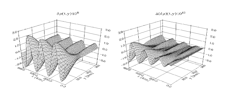
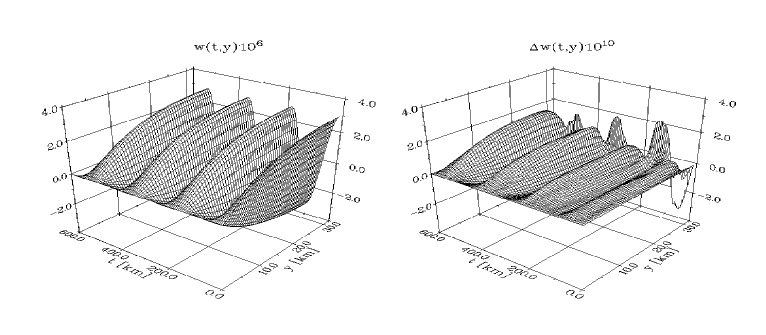
Figure 39: The left panels show the time evolution of $\delta\rho$ and $w$ obtained for neutron star model 3 with $\gamma=2.00$. The initial perturbation is given in the form of the fundamental mode in the velocity field $w$. The right panels show the deviation from the exact solution of the linearized equations.

The numerical evolution reproduces the expected harmonic time dependence with high accuracy. Because of its low frequency the fundamental mode is particularly suitable for this graphical illustration. The code reproduces the sinusoidal evolution of higher modes with comparable accuracy, but the large number of oscillations is not well resolved in plots similar to Fig. 39. For the same reason we have shown the earlier stages of the evolution up to $t=600\,\,{\rm km}$ only in the figure. The whole run lasts more than ten times longer and shows no significant loss of accuracy. It is worth mentioning that the accuracies obtained here are limited not only by the evolution code but also by the results for the static background, the eigenmode profiles and, most importantly, the eigenmode frequencies used in the calculation of the analytic solution. The same long term stability and high accuracy has been observed in similar evolutions for a variety of different neutron star models with polytropic indices $\gamma\leq 2$. Below we will see, however, that the code does not perform equally satisfactorily if we use a larger truncation density in combination with a marginally stable neutron star model with a central density just below the critical value.
For neutron star models sufficiently far away from the stability limit, we can also check the performance of the code in the linear regime by comparing the frequency spectrum of the time evolution with the values predicted by the eigenmode calculations of section 5.3.3. For this purpose initial velocity fields have been calculated for models 1 and 3 by adding the first ten eigenmode profiles whereas the initial density perturbation is set to zero. The combined amplitude of the perturbations is similar to that used above for determining the deviation from harmonic time dependence. In Fig. 40 we show the Fourier spectra for the corresponding time evolutions of the

Figure 40: The power spectra of the time evolution of the central density for neutron star models 1 and 3. The vertical bars indicate the frequencies predicted by the linear analysis.

central density perturbation $\delta\rho(t,0)$. The frequencies predicted by the eigenmode analysis are indicated by vertical bars and show good agreement with the peaks in the Fourier spectra.
Next we compare the performance of the perturbative approach with that of a “standard” non-perturbative method. We have already mentioned that we can simulate a non-perturbative approach by using vacuum flat space for the background variables. In this case we only use the TOV-model to determine the numerical grid as well as the areal radius $r$ and the sound speed $C$ as functions of $y$. The background variables, however, are specified as $\lambda=1$, $\mu=1$ and $\rho=0$. If we insert these values into the perturbative equations (5.100)-(5.109) they will become identical to the non-perturbative system (5.83)-(5.92) (after transformation to the radial coordinate $y$) with $\hat{\lambda}$, $\hat{\mu}$, $\hat{\rho}$ and $\hat{P}$ replaced by $1+\delta\lambda$, $1+\delta\mu$, $\delta\rho$ and $\delta P$. The occurrence of the constant 1 in the metric variables has no implications on the numerical performance. We have thus evolved initial data in the form of a fundamental eigenmode profile in the velocity field $w$ for neutron star model 3. First we have used the TOV-background and a resolution of 600 grid points. We have then repeated the evolution with a flat space background using 600 and 1200 grid points in order to check the dependence of the non-perturbative results on the spatial resolution. It is important to note that the same code and the same evolution algorithm has been used in both cases. The amplitude of the perturbation corresponds to an oscillation of the surface of several metres. For this amplitude we still expect the evolution to be dominated by the harmonic time dependence, although the results of section 5.3.9 below indicate the presence of weak non-linear effects. The numerical results are shown in Fig. 41, where the central density perturbation is plotted as a function of time.

Figure 41: The central density perturbation corresponding to the fundamental oscillation mode of model 3 as obtained with a perturbative method for 600 grid points (dotted curve) and a non-perturbative method for 600 (solid) and 1200 grid points (dashed curve). See text for details.

We clearly see that the perturbative evolution results in the expected sinusoidal time dependence. In the non-perturbative case the central density shows similar oscillations but simultaneously the mean value decreases significantly. In longer runs this decrease is revealed to be exponential and thus indicates a starting evaporation of the star. Neutron star model 3, however, is located on the stable branch as we can clearly see in Fig. 35 and no collapse or evaporation is expected. Indeed the higher resolution run indicates that the non-perturbative scheme converges to the harmonic solution. In order to understand this behaviour of the non-perturbative scheme we recall the presence of background terms in the evolution equation for $w_{,t}$. If we consider the coefficients $\tilde{b}_{2}$ and $\tilde{\alpha}_{21}$ given by Eqs. (5.90), (5.92), we can see that the evolution equation (5.86) contains the background in the form

$$e(y) :=\frac{1}{\mu^{2}D}\left[\frac{\lambda_{,r}}{\lambda}+\frac{C^{2}\rho_{,r}}{(\rho+P)}\right].$$ (5.161)

We know that this term vanishes by virtue of the TOV equation

Figure 42: The source terms of the evolution equation for $w$ (5.103) at the first computational step are shown for the perturbative (solid curve) and the non-perturbative scheme (dashed curve). The dotted curve shows the numerical error of the background terms and demonstrates the significance of the spurious source terms.

(5.12) and it has been removed from the equations in the perturbative formulation. In the non-perturbative case, however, it will manifest itself in the form of a residual numerical error. This error is shown in Fig. 42 for the first step in the evolution with 600 grid points together with the entire source terms of $w_{,t}$ as given by Eq. (5.86) in the non-perturbative and Eq. (5.103) in the perturbative case. Because of the cosine time dependence of the velocity the source terms should nearly vanish at $t=0$. It can be seen, however, that the source terms are dominated by the residual numerical error in the non-perturbative scheme which is particularly large at the centre and the surface. On the time scale of one oscillation period, about $150\,\,{\rm km}$, the spurious acceleration of up to $10^{-4}\,\,{\rm km}^{-1}$ will have a significant impact on the oscillation of several metres of the star. A closer investigation of the velocity field reveals that the integral effect of the residual error is an increase in the velocity field near the surface. We attribute the gradual evaporation of the star to this disturbance in the velocity field which gradually radiates matter off the numerical grid.
Considering that the same code has been used for the comparison just described, it is necessary to check the perturbative scheme for similar spurious effects. After all the main advantage of the perturbative scheme lies in higher accuracy which may postpone the onset of a spurious collapse or evaporation but not necessarily avoid it. We have already mentioned, however, that no significant deviation from the harmonic time dependence has been observed in the case of model 3 and initial data in the form of eigenmodes over very long times. In order to avoid even longer integration times and the associated computational costs, we have chosen an alternative way of testing the code for this behaviour. We use a stellar model identical to model 3 but with a central density of $\rho_{\rm c}=0.002802\,\,{\rm km}^{-2}$ which is just below the critical value given in Table 7. The initial data consist of the fundamental velocity mode with an amplitude corresponding to a surface displacement of about $10\,\,{\rm cm}$ and we use a numerical grid with 600 grid points. In the first calculation we have imposed a truncation density of $\delta\rho_{\rm s}=5\cdot 10^{-6}\,\,{\rm km}^{-2}$ and in a second run the intrinsic value of the TOV

Figure 43: The central density resulting from the evolution of the fundamental eigenmode of a neutron star corresponding to model 3 with a central density just below the critical value is plotted for a truncation density of $5\cdot 10^{-6}\,\,{\rm km}^{-2}$ (dashed curve) and $2.5\cdot 10^{-8}\,\,{\rm km}^{-2}$ (solid curve).

code $\delta\rho_{\rm s}=2.5\cdot 10^{-8}\,\,{\rm km}^{-2}$ is used. In Fig. 43 we show the resulting central density perturbation as a function of time. For the small truncation density we obtain the expected sinusoidal time dependence whereas the larger value significantly affects the evolution, even though only a fraction of $10^{-5}$ of the stellar mass has been neglected in this case. This result demonstrates the limitations of the code in its current form. For larger truncation densities it does not necessarily guarantee mass conservation which we attribute to the boundary condition (5.153) which is strictly valid only if the numerical grid extends to $\rho=0$. For sufficiently small truncation densities the resulting numerical error is negligible and has no significant effect on the evolution. For larger truncation densities, however, it can result in spurious phenomena similar to those observed in the non-perturbative case. This is particularly problematic since the investigation of non-linear effects will require perturbations of larger amplitudes and consequently larger truncation densities are necessary in order to avoid total negative energy densities. From here on we will therefore proceed in two different ways. In the remainder of section 5.3 we will investigate a simplified neutron star model for which the code ensures mass conservation for arbitrary amplitudes and negative energy densities are still avoided. This model will necessarily provide a less realistic description of a neutron star, but the general structure of the eigenmodes remains the same and it is not unrealistic to expect that non-linear effects such as mode coupling will be qualitatively similar in more realistic models. Considering the sensitivity of the numerical evolutions to the treatment of the surface, it is, however, desirable to develop a formulation of the dynamic neutron star which unambiguously provides a correct treatment of the surface. This will be done in section 5.4 where we develop a fully non-linear perturbative Lagrangian code.

5.3.7 A simplified neutron star model

In the previous section we have seen that a sufficiently large truncation density in combination with the boundary condition (5.153) may result in a continuous loss or gain of mass. In order to avoid total negative energy densities, however, we have to use sufficiently large truncation densities when we study non-linear effects in the time evolution of large amplitude perturbations. We have therefore decided to ensure mass conservation by using the alternative boundary condition

$$w =0$$ (5.162)

at the surface instead of Eq. (5.153). This means that the surface of the star remains at a fixed position in space and only fluid elements in the interior of the star are displaced during the evolution. It is the fixed location of the surface which avoids the main problems we have encountered with the Eulerian formulation so far. The model we use for the following analysis has the same equation of state as model 3 of Table 3 and a central density $\rho_{\rm c}=1.224\cdot 10^{-3}\,\,{\rm km}^{-2}$ which implies a radius $R=11.34\,\,{\rm km}$ and a total mass $M=2.18\,\,{\rm km}$. The truncation density is fixed at $\rho_{\rm s}=2.0\cdot 10^{-4}\,\,{\rm km}^{-2}$ which means that the simplified model contains $90\,\%$ of the mass of the original star and extends to $84\,\%$ of the original radius. Apart from changing the truncation density in the calculation of the TOV-background and implementing the new boundary condition in the evolution code only one further modification in the numerical setup described in section 5.3.5 is required. The outer boundary condition (5.144) in the calculation of the eigenmodes is replaced by

$$\xi(R) =0.$$ (5.163)

The resulting eigenmodes can be ordered in the same way as described in section 5.3.3 and the evolution of eigenmodes in the linear regime again results in harmonic time dependence as in the original case with the frequencies predicted by the eigenmode calculation. The first four eigenmode profiles of $\delta\rho$ and $w$ for the model mentioned above are shown in Fig. 44.

Figure 44: The profiles of the lowest four eigenmodes in $\delta\rho$ and $w$ for the simplified neutron star model.

The plots show that the number of local maxima and minima of the

Figure 45: The evolution of the central density for initial data in the form a fundamental eigenmode in the velocity field for model 3 with a central density $\rho_{\rm c}=0.002802\,\,{\rm km}^{-2}$.

profiles still corresponds to the order of the mode.

5.3.8 Testing the code with the new model

The only modification of the code that needed to be implemented for the new model is the outer boundary condition (5.162). The performance of the code in the linear regime is thus well established by the results of section 5.3.6 and we merely have to demonstrate that no spurious results are obtained for larger truncation densities. This is the only case where we will depart from the model parameters listed in the previous section and use a central density $\rho_{\rm c}=0.002802\,\,{\rm km}^{-2}$ instead. We thus recover the parameters of the model which lead to a spurious evaporation of the star in Fig. 43. For this model we have again evolved initial data in the form of the fundamental mode of the velocity with an amplitude of $10\,{\rm cm}$ using 600 grid points. In Fig. 45 we show the resulting central density $\delta\rho_{\rm c}$ together with the deviation from the harmonic solution of the linearized case. For presentation purposes we only show the evolution up to $t=6000\,\,{\rm km}$. The harmonic time dependence is reproduced with reasonable accuracy as the deviation increases linearly up to about $1\,\%$. In general we have found the eigenmode frequency the quantity most vulnerable to numerical error as can be seen for example by varying the resolution. Because of this observation and the oscillatory character of the deviation in the figure we attribute the error mainly to the limited accuracy of the frequency rather than the numerical error of the time evolution itself. The increasing phase shift between the numerical and the analytic solution arising from the limited accuracy of the frequency

Figure 46: The convergence factor obtained for evolving the second eigenmode with an amplitude of $70\,\,{\rm m}$ is shown for the variables $\delta\rho$, $w$, $\delta\lambda$ and $\delta\mu$.

will result in a linear increase of the deviation as observed in Fig. 45. In spite of the small deviation this calculation is in sharp contrast with that shown in Fig. 43, where a much smaller truncation density resulted in an exponential decay of the central density. We conclude that using a large truncation density in combination with the boundary condition (5.162) the code performs well in the linearized regime.
We now return to the model parameters of the previous section and use $\rho_{\rm c}=0.001224\,\,{\rm km}^{-2}$. In order to test the code for convergence in the non-linear regime we have evolved the second eigenmode with an amplitude corresponding to a maximal displacement of fluid elements of $70\,\,{\rm m}$. The calculation has been carried out with 400, 800 and 1600 grid points and the resulting convergence factors are shown in Fig. 46. In spite of variations around the expected value 4, the results for all variables are compatible with second order convergence.
For the next test we will use the code in the Cowling approximation, since the static metric provides a straightforward recipe to calculate conserved quantities. We have seen in section 5.3.2 that only minor modifications are required to switch between the Cowling approximation and a dynamic metric. The conservation properties with a fixed metric will therefore represent a good test for the matter evolution in the general case. The first step in the derivation of a conserved quantity is to find a time-like Killing field. The existence of such a vector field follows from the static nature of the metric in the Cowling approximation. The Killing vector can be found by looking at the Killing equation

$$\nabla_{\mu}\hbox{\vec X}_{\nu}+\nabla_{\nu}\hbox{\vec X}_{\mu} =0.$$ (5.164)

The resulting 10 differential equations can be solved rather easily and define the solution up to a constant factor. We choose this factor so that the Killing field can be written as

$$\hbox{\vec X}_{\mu} =\left[\lambda^{2},0,0,0\right].$$ (5.165)

The conserved quantity then follows from contraction of the Killing field with the energy momentum tensor

$$\hbox{\vec J}^{\mu} =\hbox{\vec{T}}^{\mu\nu}\hbox{\vec X}_{\nu}.$$ (5.166)

By virtue of conservation of energy momentum this vector satisfies the condition

$$\nabla_{\mu}\hbox{\vec J}^{\mu} =0.$$ (5.167)

With the metric (5.2) and the energy momentum tensor

Figure 47: The numerical evolution of the function $E$ obtained in the Cowling approximation. The quantity is conserved with an accuracy better than $10^{-4}$.

(5.78) this equation can be written in conservative form

$$\partial_{t}\left(\lambda\mu r^{2}\hbox{\vec J}^{t}\right)+\partial_{r}\left(\lambda\mu r^{2}\hbox{\vec J}^{r}\right) =0,$$ (5.168)

where the $t$ and $r$ components of J are given by

$$\hbox{\vec J}^{t} =(1+\mu^{2}w^{2})\hat{\rho}+\mu^{2}w^{2}\hat{P},$$ (5.169)

$$\hbox{\vec J}^{r} =\frac{w}{v}(1+\mu^{2}w^{2})(\hat{\rho}+\hat{P}).$$ (5.170)

If we consider a general conservation law in one dimension

$$u_{,t}+F(u)_{,r} =0,$$ (5.171)

we obtain after integration over $t$ and $r$

$$\int_{0}^{R}{[u(T,r)-u(0,r)]}dr+\int_{0}^{T}{[F(t,R)-F(t,0)]}dr =0.$$ (5.172)

In our case the flux function is given by $F=\lambda\mu r^{2}\hbox{\vec J}^{r}$ and vanishes at $r=0$ and $r=R$ because the velocity $w$ vanishes at both boundaries. Consequently

$$E =\int_{0}^{R}{\lambda\mu r^{2}\hbox{\vec J}^{t}}dr$$ (5.173)

is a conserved quantity.
In order to test the conservation properties of the code we have evolved the same initial data as in the convergence analysis with the metric fixed at the background values. In Fig. 47 we show $E$ as a function of time as calculated with 800 grid points. The quantity is conserved with a relative accuracy better than $10^{-4}$. Even higher accuracy is obtained for smaller amplitudes of the initial data. We have thus demonstrated that the code performs well in the linear as well as the non-linear regime. The applicability of the code to a wide range of amplitudes will be crucial when we study non-linear effects in the evolution of eigenmodes in the next subsection.

5.3.9 Non-linear mode coupling

(a) Measuring the eigenmode coefficients
We will now use the simplified neutron star model described in section 5.3.7 to study the coupling of eigenmodes in non-linear evolutions of radial oscillations. In order to measure the presence of the individual eigenmodes in the evolution we recall the Sturm-Liouville problem (5.118) which determines the eigenmode solutions in terms of the rescaled displacement vector $\zeta$. In section 5.3.3 we have seen that the solutions $\zeta_{i}$ form a complete orthonormal system with respect to the inner product defined in Eq. (5.122). This property enables us to quantify the contributions of the different eigenmodes in the evolution at any given time. We need to calculate the displacement $\zeta(t,r)$ of a fully non-linear evolution from the fundamental variables $\delta\rho$ and $w$. For this purpose we eliminate $\xi$ from Eqs. (5.111) and (5.112) and obtain

$$\zeta_{,t} =r^{2}w.$$ (5.174)

The initial values of $\zeta$ follow from the initial data which we provide in the form of an eigenmode in the velocity field $w$ and zero energy density perturbation $\delta\rho$. We can see from Eq. (5.130) that the initial displacement $\zeta$ vanishes as a consequence. At any time $t$ we can then expand the non-linear displacement $\zeta(t,r)$ in terms of the eigenmodes

$$\zeta(t,r) =\sum_{i}{A_{i}(t)\zeta_{i}(r)},$$ (5.175)

where the time dependent coefficients are given by the inner product

$$A_{i}(t) =\langle\zeta(t,r),\zeta_{i}(r)\rangle.$$ (5.176)

In practice we prefer to calculate the eigenmode coefficients from the time derivative of this equation

$$\frac{\partial A_{i}}{\partial t} =\langle\zeta_{,t},\zeta_{i}\rangle,$$ (5.177)

where we have dropped the $t$ and $r$ dependence for convenience. If we substitute Eq. (5.174) for $\zeta_{,t}$ we obtain the final result

$$\frac{\partial A_{i}}{\partial t} =\langle r^{2}w,\zeta_{i}\rangle.$$ (5.178)

We can thus calculate the time derivative of the coefficients and use the initial values to obtain the coefficients at any given time $t$. In our case all coefficients are zero initially because of the vanishing of $\zeta$. The integral appearing in the definition of the inner product is calculated with the fourth order Simpson method (see for example Press1989).
It is also interesting to consider the relative coefficients defined by

$$R_{i}(t) =\frac{\langle\zeta,\zeta_{i}\rangle}{\langle\zeta,\zeta\rangle},$$ (5.179)

whenever $\zeta$ is a non-zero function. If we multiply this equation

Figure 48: The sum of the first ten $R_{i}$ has been calculated for evolving the second eigenmode with an amplitude of $70\,\,{\rm m}$.

by $A_{i}$ and sum over $i$, we can use Eq. (5.175) to obtain the relation

$$\sum_{i}{R_{i}} =1,$$ (5.180)

which can be used to check the completeness of the numerically calculated eigenmodes. For this purpose we have evolved the second eigenmode with a large amplitude corresponding to a maximum displacement of $70\,\,{\rm m}$ and calculated the sum of the first ten weighted coefficients $R_{i}$ using 600 grid points. The result is shown in Fig. 48 and demonstrates that Eq. (5.180) is satisfied to within less than one per cent. This does not only confirm the completeness of the system of eigenmodes, but also indicates that the energy essentially remains within the lowest ten eigenmodes. In order to check the orthonormality we have calculated the inner products of the eigenmodes. The results for the lowest five eigenmodes are shown in Table 9 and demonstrate that

Table 9: The inner product $\langle\zeta_{i},\zeta_{j}\rangle$ between the five lowest eigenmodes.

	$\zeta_{1}$	$\zeta_{2}$	$\zeta_{3}$	$\zeta_{4}$	$\zeta_{5}$
$\zeta_{1}$	1.0	$-2.1\cdot 10^{-6}$	$-6.3\cdot 10^{-6}$	$-1.2\cdot 10^{-6}$	$-2.6\cdot 10^{-6}$
$\zeta_{2}$	$-2.1\cdot 10^{-6}$	1.0	$-8.0\cdot 10^{-6}$	$-1.5\cdot 10^{-5}$	$-6.3\cdot 10^{-6}$
$\zeta_{3}$	$-6.3\cdot 10^{-6}$	$-8.0\cdot 10^{-6}$	1.0	$-1.8\cdot 10^{-5}$	$-2.7\cdot 10^{-5}$
$\zeta_{4}$	$-1.2\cdot 10^{-6}$	$-1.5\cdot 10^{-5}$	$-1.8\cdot 10^{-5}$	1.0	$-3.2\cdot 10^{-5}$
$\zeta_{5}$	$-2.6\cdot 10^{-6}$	$-6.3\cdot 10^{-6}$	$-2.7\cdot 10^{-5}$	$-3.2\cdot 10^{-5}$	1.0

the orthonormality condition (5.125) is satisfied with high accuracy.

(b) Non-linear coupling between eigenmodes
In order to study the coupling of modes due to non-linear effects we have provided initial data in the form of one velocity eigenmode. The order of the eigenmode $j$ and the amplitude of the initial data $K_{j}$ are free parameters that determine the physical setup. We will specify the amplitude of the initial perturbation by the maximum value of the eigenmode profile of the displacement vector $\xi$ corresponding to the initial velocity perturbation. This is a measure for the maximum displacement a fluid element of the interior of the star will undergo. During the evolution we calculate the eigenmode coefficients $A_{i}(t)$ with $1\leq i\leq 10\,\,{\rm or}\,\,15$ according to the method described above. Due to the oscillatory character of the modes, the coefficients will also oscillate during the evolution. This is shown in Fig. 49 where we plot the coefficients $A_{2}(t)$ and $A_{4}(t)$ for evolving the second eigenmode. A large amplitude corresponding to a maximum displacement of $70\,\,{\rm m}$ has been used

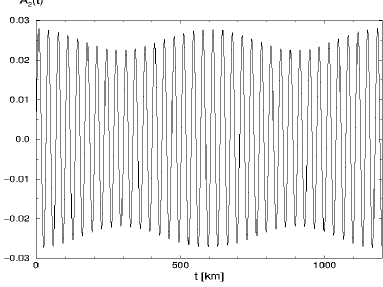
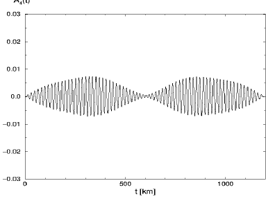
Figure 49: The coefficients $A_{2}(t)$ and $A_{4}(t)$ obtained for initial data in the form of the second eigenmode with an amplitude of $70\,{\rm m}$.

for this calculation and we can clearly see the transfer of energy between the second and the fourth mode. It is interesting to see that the energy transferred to the fourth mode does not remain there but instead is periodically passed back and forth between the two modes. We observe a qualitatively similar behaviour for the other eigenmodes, although these are excited less efficiently. If we want to investigate this coupling between eigenmodes more systematically, we need to quantify the degree to which a particular mode has been excited in an evolution. For this purpose we will use the maximum value of the corresponding coefficient obtained during that evolution. We will refer to these maxima by $A_{i}$ as opposed to $A_{i}(t)$ used for the time dependent coefficients. We have thus evolved the eigenmodes $i=1$, 2 and 3, referred to

Figure 50: The eigenmode coefficients for the first ten eigenmodes are shown as a function of the amplitude $K_{1}$ for initial data in the form of the fundamental velocity mode.

as case 1, 2 and 3 from now on, with amplitudes ranging between $1\,\,{\rm cm}$ and $100\,\,{\rm m}$. At some stage in the range between about $50\,{\rm m}$ and $100\,{\rm m}$ we observed the onset of shock formation. The accuracy of the eigenmode coefficients resulting from these evolutions is not clear. In this discussion we have therefore only used amplitudes for which no discontinuities are observed.

Figure 51: The excitation of eigenmodes has been fitted with quadratic power laws in the range between $K_{1}=1\,\,{\rm m}$ and $10\,\,{\rm m}$.

For the numerical runs we have used 3200 grid points and an integration time of $1500\,\,{\rm km}$. Test runs over significantly longer times did not lead to significantly different results for the $A_{i}$ which is compatible with the periodic exchange of energy shown in Fig. 49. The high grid resolution on the other hand enables us to measure small eigenmode coefficients with good accuracy.

Case 1:
We start our analysis with case 1, where the fundamental mode is excited initially. In Fig. 50 we plot the coefficients $A_{i}$ as a function of the initial amplitude $K_{1}$ for the first ten

Figure 52: The eigenmode coefficients $A_{2}$, $A_{3}$ and $A_{4}$ are fitted with linear combinations of power laws according to Eqs. (5.183)-(5.185).

eigenmodes. We find that the coefficient $A_{1}$ increases linearly with the amplitude $K_{1}$ as expected. A closer investigation of the higher eigenmode coefficients, however, reveals the presence of two distinct regimes.

• In a weakly non-linear regime for amplitudes up to about $10\,\,{\rm m}$ all coefficients $A_{2},\ldots A_{10}$ increase quadratically with the amplitude $K_{1}$. Deviations from this quadratic power law at very small amplitudes are due to the limited numerical accuracy in calculating the coefficients.

• At larger amplitudes all eigenmode coefficients except for $A_{2}$ show a transition to power laws with larger exponent which marks a moderately non-linear regime.

We have illustrated this behaviour in Fig. 51 where the eigenmode coefficients have been approximated with quadratic power laws

$$A_{i} =c_{i}\cdot K_{1}^{\,\,2}.$$ (5.181)

The coupling coefficients $c_{i}$ which represent the coupling strength in the weakly non-linear regime have been obtained from least square fits of quadratic power laws to the eigenmode coefficients in amplitude ranges between $0.1\,\,{\rm m}$ and $10\,\,{\rm m}$. It is interesting to investigate the dependence of the coupling coefficients on the order of the eigenmodes. This is shown in the upper left panel of Fig. 53, where we plot $c_{i}$ over the order $i-1$.

Figure 53: The coupling coefficients $c_{i}$ defined in Eq. 5.181 are plotted as a function of the mode number $i-1$ for case 1 in the upper left panel. In the upper right and lower panel we plot the corresponding coefficients for case 2 and 3 as a function of the mode number $i-3$ and $i-5$ respectively. In all cases the coefficients can be approximated with inverse cubic power laws as indicated by the solid lines.

The solid line in this figure shows a power law fit for these coupling coefficients given by

$$c_{i} =3.2\cdot 10^{-7}\cdot(i-1)^{-3}.$$ (5.182)

This result is compatible with the expectation that $c_{i}\rightarrow 0$ as $i\rightarrow\infty$. Otherwise an infinite number of modes would each be excited with a finite amount of energy. In the moderately non-linear regime the eigenmode coefficients $A_{3},\ldots,A_{10}$ show a higher order growth with the amplitude $K_{1}$. For the most efficiently excited modes 2, 3 and 4 we have been able to approximate the eigenmode coefficients with the following combinations of power laws

$$A_{2} =3.6\cdot 10^{-7}\cdot K_{1}^{\,2},$$ (5.183)

$$A_{3} =3.4\cdot 10^{-8}\cdot K_{1}^{2}+9.7\cdot 10^{-10}\cdot K_{1}^{3},$$ (5.184)

$$A_{4} =1.0\cdot 10^{-8}\cdot K_{1}^{2}+1.2\cdot 10^{-11}\cdot K_{1}^{4}.$$ (5.185)

Here the higher order power laws have been obtained from fitting the eigenmode coefficients after subtracting the quadratic contributions. The resulting fits are shown in Fig. 52. The higher order contributions for the higher eigenmodes is rather weak so that it is difficult to obtain accurate measurements of the

Figure 54: The eigenmode coefficients for the first ten eigenmodes are shown for initial data in the form of the second velocity mode.

corresponding power law exponents. It is thus not clear whether the regular pattern suggested by Eqs. (5.183)-(5.185) remains valid for higher modes. The steepening of the curves in the

Figure 55: The excitation of eigenmodes in case 2 has been fitted with quadratic power laws in the range between $K_{1}=0.1\,\,{\rm m}$ and $10\,\,{\rm m}$.

moderately non-linear regime, however, can be clearly seen in Fig. 51.

Case 2:
We will now address the question to what extent these results remain valid if we initially excite higher modes. For this purpose we have repeated the

Figure 56: In the upper panel we show the higher order power law contributions of Eqs. (5.186)-(5.189) which fit the even eigenmode coefficients rather well in the moderately non-linear regime. The lower panel shows the resulting fits obtained from the sum of the quadratic and the higher order power laws according to the same equations.

numerical analysis by providing initial data in the form of the second velocity mode. The resulting eigenmode coefficients are shown as a function of the amplitude $K_{2}$ in Fig. 54. The presence of the two distinct regimes is again clearly demonstrated by the figures and a closer investigation confirms the quadratic growth of the eigenmode coefficients in the weakly non-linear regime. This is demonstrated in Fig. 55 where the corresponding quadratic power law fits are shown for the eigenmodes. We also observe a similar dependence of the quadratic coupling coefficients $c_{i}$ on the mode number. In case 1 we observed a power law relation given by Eq. (5.182) between the coefficients $c_{i}$ and the mode number $i-1$. In case 2 we can also approximate the coefficients $c_{i}$ reasonably well with an inverse cubic power law if we use the number $i-3$ instead which is demonstrated in the right panel of Fig. 53. The lower order modes 1 and 3 do not fit into this pattern and we shall readdress their behaviour in the quadratic regime below when we discuss case 3.
Apart from these similarities there are some interesting differences between case 1 and case 2:

• The transition from the weakly to the moderately non-linear regime occurs at smaller amplitudes than in case 1. This is particularly pronounced in the case of mode 6 (see Fig. 55).

• The regular pattern observed in case 1 in the moderately non-linear regime for the strongly excited modes 2, 3 and 4, which is expressed in Eqs. (5.183)-(5.185), is now being observed for the eigenmodes of even order $2n$. We obtain excellent fits for the data if we model the even eigenmode coefficients with the following linear combinations of power laws.

  $$A_{4} =1.9\cdot 10^{-6}\cdot K_{1}^{2},$$ (5.186)

  $$A_{6} =2.5\cdot 10^{-8}\cdot K_{1}^{2}+8.7\cdot 10^{-9}\cdot K_{1}^{3},$$ (5.187)

  $$A_{8} =4.9\cdot 10^{-9}\cdot K_{1}^{2}+6.2\cdot 10^{-11}\cdot K_{1}^{4},$$ (5.188)

  $$A_{10} =1.8\cdot 10^{-9}\cdot K_{1}^{2}+4.9\cdot 10^{-13}\cdot K_{1}^{5}.$$ (5.189)

  In Fig. 56 we show the curves resulting from the higher order power laws as well as those corresponding to the linear combinations. For the odd modes the higher order contributions are rather small so that we cannot accurately measure the corresponding power law indices. The steepening of the curves and thus the onset of the moderately non-linear regime, however, is clearly visible.

• Whereas the quadratic coupling coefficients $c_{i}$ shown in the right panel of Fig. 53 show a continuous decrease with the order of the mode starting with mode 4, a clear preference of the second mode to couple to modes of even order $2n$ is observed in the moderately non-linear regime. This is indicated by the rather efficient coupling to mode 4 and the significantly steeper increase of the eigenmode coefficients $A_{6}$, $A_{8}$ and $A_{10}$ for larger amplitudes $K_{2}$ in Fig. 55.

• A small flattening of the even eigenmode coefficients at large amplitudes in Fig. 56 may indicate the onset of saturation effects. A possible mechanism for saturation is the formation of discontinuities. As we have already mentioned we have chosen an amplitude range in which no shock formation is observed. At the high end of our amplitude range, it may be possible, however, that similar dissipative effects due to the strong non-linearity start having an effect on the coupling of eigenmodes.

Case 3:
Next we consider case 3 where we perturb the star with the third velocity mode. The fundamental observations we have made in the previous two cases

Table 10: The quadratic coupling coefficients $c_{i}$ for the lower modes in case 3.

$i$	$c_{i}$
1	$2.0\cdot 10^{-7}$
2	$1.2\cdot 10^{-7}$
4	$6.7\cdot 10^{-8}$
5	$3.0\cdot 10^{-8}$

are confirmed by the results in this case. In the weakly non-linear regime all eigenmode coefficients (except for $A_{3}$) grow quadratically with the amplitude $K_{3}$. The corresponding quadratic coupling coefficients can once more be approximated with a power law with exponent $-3$. We find, however, that the relevant mode number is now $i-5$. This behaviour is graphically illustrated in the lower panel of Fig. 53 where the coupling coefficients are shown together with the power law approximation. The results of this figure suggest the following regular pattern: For initial data in the form of eigenmode $j$ the quadratic coupling coefficients starting with mode $2j$ are well approximated by an inverse cubic power law of a relative mode number $i+1-2j$ which is $1$ for mode $2j$, $2$ for mode $2j+1$ and so on.
We still have to analyse the quadratic coupling coefficients of the modes below $2j$. In case 1 and 2 we did not have enough data to derive any results for these modes. For case 3 we have listed the corresponding coefficients $c_{i}$ in Table 10. The coefficients $c_{i}$ are approximately reduced by a factor of 2 each time the mode number is increased which may indicate an exponential decrease of the quadratic coupling coefficients for the low order modes.

Figure 57: The eigenmode coefficient $A_{3}$, $A_{6}$,$\ldots$,$A_{15}$ are shown for case 3 together with the resulting fits according to Eqs. (5.190)-(5.193).

This is only a vague conclusion from a small data set, however, and needs to be confirmed by studies of higher eigenmodes.
In the moderately non-linear regime we have seen for case 2 a preferred coupling to modes with an even order $2n$. In analogy we find that the third eigenmode couples more efficiently to modes of order $3n$ for larger amplitudes. Again we can approximate the results with good accuracy with combinations of two power laws analogous to Eqs. (5.186)-(5.189)

$$A_{6} =1.2\cdot 10^{-6}\cdot K_{3}^{2},$$ (5.190)

$$A_{9} =0.9\cdot 10^{-8}\cdot K_{3}^{2}+6.5\cdot 10^{-9}\cdot K_{3}^{3},$$ (5.191)

$$A_{12} =2.2\cdot 10^{-9}\cdot K_{3}^{2}+4.6\cdot 10^{-11}\cdot K_{3}^{4},$$ (5.192)

$$A_{15} =7.8\cdot 10^{-10}\cdot K_{3}^{2}+4.5\cdot 10^{-13}\cdot K_{3}^{5}.$$ (5.193)

We recognise the same pattern of increasing integer power law indices in the higher order terms that we have already found in case 1 and 2. These results are graphically illustrated in Fig. 57. Again the higher order contributions in the other eigenmodes is clearly present but too weak to facilitate an accurate measurement of the exponents.
We conclude the study of non-linear mode coupling with a summary of the key results.

• We clearly observe two distinct regimes in the non-linear coupling of eigenmodes. In the weekly non-linear regime, normally up to amplitudes of several metres, all eigenmode coefficients grow quadratically with the amplitude $K_{j}$. In the moderately non-linear regime we observe a steeper increase of the coefficients $A_{i}$.

• In the quadratic regime the coupling coefficients $c_{i}$ generally decrease with increasing order of the eigenmodes. If the initial perturbation is given in the form of mode $j$, we can model the behaviour of the quadratic coupling coefficients with an inverse cubic power law of the mode number starting with mode $2j$. The coupling to lower modes does not obey the same pattern, but we also observe a decrease of the $c_{i}$ with increasing mode number for these modes. This decrease may have exponential character.

• In the moderately non-linear regime an initially present mode $j$ shows a preference to couple to modes of order $n\cdot j$ where $n\geq 2$ is an integer number. In these cases we can accurately model the dependence of the eigenmode coefficients on the amplitude $K_{j}$ with the sum of a quadratic and a higher order power law with exponent $n$: $A_{i}=c_{i}\cdot K_{j}^{\,2}+d_{i}\cdot K_{j}^{\,n}$ for $i=n\cdot j$.

• In some cases we observe a flattening of the eigenmode coefficients at amplitudes of about $50\,{\rm m}$ which may indicate the onset of saturation.

5.3.10 Discussion of the non-linear mode-coupling

In the previous section we have studied the coupling of eigenmodes due to non-linear effects by evolving a single eigenmode with varying amplitude. Concerning the transfer of energy to other modes we have found two distinct regimes, a weakly non-linear regime where the excitation of modes grows quadratically with the initial amplitude and a moderately non-linear regime, where this increase can be reasonably well described by power laws of higher order.
In the analytic study of non-linear mode coupling one normally views the eigenmode coefficients as harmonic oscillators and the non-linear interaction between eigenmodes is represented in the form of driving terms which are quadratic or of higher order in the amplitudes (see for example VanHoolst1996)

$$\frac{d^{2}A_{i}}{dt^{2}}+\omega_{i}^{2}A_{i} =c_{i}^{jk}A_{j}A_{k}+d_{i}^{jkl}A_{j}A_{k}A_{l}+\ldots,$$ (5.194)

where the $c_{i}^{jk}$, $d_{i}^{jkl},\ldots$ are the quadratic, cubic and higher order coupling coefficients and summation over $j,k,l$ is assumed. In our analysis the initial data consists in one isolated eigenmode $j$, so that the right hand side can be approximated by $c_{i}A_{j}^{2}+d_{i}A_{j}^{3}+\ldots$ In analytic studies this series expansion is normally truncated at second or third order. In view of our results the omission of higher order terms seems to be justified in the weakly non-linear regime, where our fully non-linear simulations confirm that quadratic terms in the initial amplitude dominate the coupling between eigenmodes. This is no longer true, however, in the moderately non-linear regime, where higher order terms are more important. In particular the regular pattern suggested for example by Eqs. (5.186)-(5.189) indicates that the excitation of higher order modes is dominated by increasingly higher order powers of the initial amplitude. It is not clear how this behaviour can be modelled in the framework of a finite series expansion of the type (5.194). It rather seems that the use of fully non-linear methods such as the numerical technique described in this work is necessary in order to obtain a comprehensive description of the coupling between eigenmodes in the moderately non-linear regime. In terms of the maximum displacement of fluid elements in the star this corresponds to initial amplitudes as low as a couple of metres.
We have also observed that given an initial mode $j$ the coupling to modes $n\cdot j$ is particularly efficient in the moderately non-linear regime. We interprete this as a resonance effect, which we illustrate in the simple case of a forced oscillator

$$\frac{d^{2}A_{i}}{dt^{2}}+\omega_{i}^{2}A_{i}=F\sin{\Omega t},$$ (5.195)

where $\Omega$ is the frequency and $F$ the amplitude of the external force. The particular integral of this ordinary differential equation is

$$A_{i}(t) =\frac{F}{\omega_{i}^{2}-\Omega^{2}}\sin{\Omega t},$$ (5.196)

which implies resonance if $\omega_{i}=\Omega$. If we assume that resonance occurs for any integer multiple of the frequency $\Omega$ in the general non-linear case, we can schematically write the eigenmode coefficients in the form

$$A_{i}(t) =\sum_{n}\frac{F_{n}}{\omega_{i}^{2}-(n\Omega)^{2}},$$ (5.197)

where the $F_{n}$ may depend on the frequencies. The analytic study of non-linear mode coupling up to cubic order leads to eigenmode coefficients which resemble this pattern [see for example Eqs. (18), (19) of VanHoolst1996]. In our case the external force is provided by the non-linear coupling to the initial mode $j$, so that $\Omega=\omega_{j}$. We therefore obtain resonance in Eq. (5.197) if $\omega_{i}=n\omega_{j}$. As can be seen for example in Fig. 40, the eigenfrequencies of radial neutron star oscillations are fairly equally spaced in the frequency domain with the exception of the fundamental mode and we can reasonably well approximate $\omega_{i}\approx(i\omega_{j})/j$ for $i,j\geq 2$. The condition for resonance then becomes

$$i =n\cdot j,$$ (5.198)

which is exactly the relation we have observed in section 5.3.9.
From the relativistic point of view the non-linear coupling of eigenmodes in the weak and moderately non-linear regime is of particular interest in the discussion of unstable modes of rotating neutron stars. The underlying principle of these unstable oscillation modes is the increase in amplitude of the oscillation due to the emission of gravitational waves. The increased amplitude in turn gives rise to stronger gravitational radiation and so on. The conservation of energy is ensured in this case by the spin-down of the neutron star and the resulting decrease of rotational energy which sets a natural upper limit on this run-away effect. The physical mechanism which facilitates this remarkable instability is known as the CFS-instability (Chandrasekhar1970, Friedman1978). In order for a neutron star oscillation mode to be subject to the CFS-instability two conditions must be satisfied: (1) the mode must be retrograde with respect to the star but prograde with respect to a distant inertial observer and (2) the energy loss in the rotating frame due to dissipative effects must be smaller than the amount of energy gained from the gravitationally driven instability. The particular importance of the so-called $r$-modes in this respect arises from the fact that the dominating $l=m=2$ $r$-mode satisfies the first CFS-condition for arbitrarily small values of the angular frequency of the neutron star (Andersson1998). One of the most important questions raised in connection with the $r$-modes concerns the efficiency with which energy is dissipated for example due to viscosity or non-linear effects.
Considering the gradual increase in the oscillation amplitude, it is important to understand how the instability of the mode is affected in the weakly non-linear regime. To our knowledge the numerical studies presented in this work provide the first fully non-linear time evolutions of neutron star oscillations with high accuracy for amplitudes going all the way down to the weakly non-linear regime. Our results may therefore pave some of the way towards understanding non-linear effects in a wider class of neutron star oscillations. In particular we have managed to quantify the transfer of energy from low into higher eigenmodes. The picture that emerges from these evolutions is that only a rather small fraction of energy is shifted away from the low eigenmodes. In particular the results shown in Fig. 49 indicate that the energy shifted towards higher eigenmodes does not accumulate in time but is rather transferred back and forth between the initially present and the higher mode. Correspondingly we do not observe an efficient cascade of energy into higher modes. It is not clear, however, to what extent this picture will change if the energy residing in the higher order modes is gradually dissipated. In the context of $r$-modes it is expected that the energy in higher order modes is dissipated on a much shorter timescale than that of the dominating $l=m=2$ mode. The numerical techniques and the code developed in this work may facilitate a corresponding study in the framework of radial oscillations by introducing an artificial damping of higher order modes and an external force which drives the fundamental mode. One may then look for steady state situations arising from this model, where the amount of energy transfered to higher modes and thus dissipated equals that gained from the external driving mechanism.
From a numerical point of view we emphasise the new perturbative approach which enabled us to obtain highly accurate fully non-linear evolutions over a large range of amplitudes. This technique can be applied for any physical problem where there exists a non-trivial static limit. The dynamic evolution can always be considered a finite perturbation of the static case and a corresponding perturbative formulation will provide a numerical accuracy that is determined by the amplitude of the perturbation rather than the static background. We expect this method to be particularly effective in higher dimensional evolutions where the grid resolution is rather limited by computational costs and the ensuing residual error arising from background terms in a non-perturbative formulation will be more significant.

5.4 Radial oscillations in a Lagrangian formulation

In the previous section we have seen that an Eulerian description of radial oscillations encounters difficulties at the stellar surface for several reasons. For certain equations of state the eigenmode profiles predicted by the linearized theory result in a diverging energy density perturbation. A purely numerical problem arises from the movement of the stellar surface with respect to the numerical grid. Highly sophisticated techniques may be required to adequately describe the surface of a neutron star in Eulerian coordinates and it is not clear to what extent these will lead to a fully satisfactory performance in the linear regime where the exact solution is known to high accuracy and facilitates a quantitative test for the code. It is interesting to see that these problems vanish immediately once the problem is described in a formalism where the coordinates follow the movement of the fluid elements. Even though it is not obvious how to generalise a Lagrangian approach to scenarios in two or three spatial dimensions, it still seems to be the natural choice for the 1-dimensional case. Lagrangian codes have often been based on the formulation of May1966 and May1967 who following Misner1964 use a vanishing shift vector and define the radial coordinate in terms of the interior rest mass. In order to facilitate a simple comparison with the Eulerian code discussed in section 5.3, however, it will be convenient for us to use as similar a gauge choice to the Eulerian case as possible. For this purpose we will follow Schinder1988 and use a Lagrangian gauge in combination with the polar slicing condition which is also implemented in the Eulerian code (cf. section 5.3.1). As a particularly useful consequence the singularity avoiding properties of this condition in combination with the Lagrangian gauge make this code highly suitable for studying spherically symmetric gravitational collapse. We will not exhaustively study this type of scenarios in this work, but will use the analytic solution by Oppenheimer1939b which describes the collapse of a homogeneous dust sphere for testing the code.

5.4.1 The equations in the Lagrangian formulation

The derivation of the Lagrangian equations for a dynamic spherically symmetric neutron star was largely inspired by the work of Schinder1988. We will, however, slightly deviate from their approach and work with a different set of variables and equations.
We start by considering the line element of a spherically symmetric space time in polar slicing and Lagrangian gauge. As a result of the polar slicing condition, we are able to choose the same time coordinate $t$ as in the Eulerian case. The radial coordinate $x$ will label the fluid elements and generally differ from the areal radius $r$ which is intrinsically not comoving with the matter. Finally we choose standard angular coordinates $\theta$ and $\phi$ as above. Below we will see that the polar slicing condition implies a non-vanishing shift vector so that the line element becomes

$$ds^{2} =\left(-\hat{\lambda}^{2}+\frac{\hat{\Gamma}\beta^{2}}{\hat{r}_{,x}^{2}}\right)dt^{2}+2\beta dt\,dx+\frac{\hat{r}_{,x}^{2}}{\hat{\Gamma}}dx^{2}+\hat{r}^{2}(d\theta^{2}+\sin^{2}{\theta}d\phi^{2}).$$ (5.199)

It turns out to be convenient for our discussion if we introduce the variables

$$w =\frac{\hat{r}_{,t}}{\hat{\lambda}},$$ (5.200)

$$\Omega^{2} =\hat{\Gamma}-w^{2},$$ (5.201)

$$\hat{m} =\frac{\hat{r}}{2}(1-\hat{\Gamma}),$$ (5.202)

where the velocity is identical to that used in the Eulerian case. As before we use the “hat” to distinguish between the time dependent variables and their counterparts in the static case. We note that we need to distinguish between the time dependent areal radius $\hat{r}$ and the static value $r$, since the areal radius corresponding to the position of a fluid element is a dependent variable and will generally vary with time. In the Eulerian case the areal radius was a coordinate and therefore intrinsically independent of time. If we compare the Lagrangian line element (5.199) with the Eulerian one given by Eq. (5.77) we therefore have to use the time dependent $\hat{r}$ in the latter line element instead of $r$. The coordinate transformation relating the two line elements is described by

$$\hat{r} =\hat{r}(t,x).$$ (5.203)

The transformation law for the metric components corresponding to the transformation from coordinates $\hbox{\vec$x$}^{\mu}=(t,x,\theta,\phi)$ to $\hbox{\vec$x$}^{{}^{\prime}\mu}=(t,r,\theta,\phi)$ is given by

$$\hbox{\vec g}^{\prime}_{\mu\nu} =\frac{\partial\hbox{\vec$x$}^{\rho}}{\partial\hbox{\vec$x$}^{{}^{\prime}\mu}}\frac{\partial\hbox{\vec$x$}^{\sigma}}{\partial\hbox{\vec$x$}^{{}^{\prime}\nu}}\hbox{\vec g}_{\rho\sigma},$$ (5.204)

and leads to the two non-trivial equations

$$\beta =\hat{r}_{,x}\hat{r}_{,t}\hat{\mu}^{2},$$ (5.205)

$$\hat{\Gamma} =\frac{1}{\hat{\mu}^{2}}.$$ (5.206)

As a consequence the shift vector $\beta$ is related to the components of the Lagrangian metric by

$$\beta=\hat{\lambda}\frac{w\,\hat{r}_{,x}}{\hat{\Gamma}}.$$ (5.207)

In terms of the extrinsic curvature defined in Eq. (2.19) this relation can be written as $\hbox{\vec{K}}^{\theta}_{\,\,\,\theta}=\hbox{\vec{K}}^{\phi}_{\,\,\,\phi}=0$ and we have recovered the polar slicing condition. The non-vanishing shift vector (5.207) is the price we have to pay for keeping the polar slicing condition in the Lagrangian gauge.
As far as the matter is concerned, we use again a single component perfect fluid and thus the energy momentum tensor given by Eq. (5.78). Since the fluid elements do not move with respect to the radial coordinate $x$, the 4-velocity has zero spatial components and is determined by the normalisation $\hbox{\vec u}^{\mu}\hbox{\vec u}_{\mu}=-1$

$$\hbox{\vec u}^{\mu} =\left(\frac{\sqrt{\hat{\Gamma}}}{\hat{\lambda}\Omega},0,0,0\right).$$ (5.208)

The resulting field equations $\hbox{\vec{G}}_{\mu\nu}=8\pi\hbox{\vec{T}}_{\mu\nu}$ can be written as

$$\frac{\hat{\lambda}_{,x}}{\hat{\lambda}} =\frac{\hat{r}_{,x}}{\hat{r}\hat{\Gamma}}\left(\frac{\hat{m}}{\hat{r}}+4\pi\hat{r}^{2}\frac{w^{2}\hat{\rho}+\hat{\Gamma}\hat{P}}{\Omega^{2}}\right),$$ (5.209)

$$\hat{m}_{,x} =4\pi\hat{r}^{2}\hat{r}_{,x}\frac{\hat{\Gamma}\hat{\rho}+w^{2}\hat{P}}{\Omega^{2}},$$ (5.210)

$$\hat{m}_{,t} =-4\pi\hat{r}^{2}\hat{\lambda}w\hat{P}.$$ (5.211)

Similarly the conservation of energy and momentum $\nabla_{\mu}\hbox{\vec{T}}^{\mu}_{\,\,\,\,{\nu}}=0$ leads to two evolution equations for the matter variables

$$\hat{\rho}_{,t}+(\hat{\rho}+\hat{P})\frac{\Omega}{\hat{r}^{2}\hat{r}_{,x}}\left(\frac{\hat{r}^{2}\hat{r}_{,x}}{\Omega}\right)_{,t}=0,$$ (5.212)

$$\Omega^{4}\frac{\hat{P}_{,x}}{\hat{r}_{,x}}+\hat{P}_{,t}\frac{w}{\hat{\lambda}}\Omega^{2}+(\hat{\rho}+\hat{P})\left[\hat{\gamma}\frac{w_{,t}}{\hat{\lambda}}+(\hat{\gamma}-2w^{2})\left(\frac{\hat{m}}{\hat{r}^{2}}+4\pi\hat{r}\hat{P}\right)\right]=0,$$ (5.213)

and the system is closed by the polytropic equation of state (5.79). It is worth pointing out that the appearance of the time derivative in the field equation (5.211) does not contradict the absence of gravitational degrees of freedom in spherical symmetry. This equation can be shown to be a consequence of the constraints (5.209), (5.210) and the matter equations (5.212), (5.213). In this sense the degrees of freedom still reside in the matter variables and the metric is determined at each time irrespective of its history. In practice, however, we will use the rather simple equation (5.211) to evolve the variable $\hat{m}$ instead of evolving $\hat{\rho}$ via the matter equation (5.212).
If we consider the static limit of the system of equations (5.209)-(5.213) we expect to recover the Tolman-Oppenheimer-Volkoff equations (5.48)-(5.51). That this is indeed the case can be seen if we set all time derivatives including the velocity $w$ to zero and assume that $x$ is identical to the coordinate $x$ we used in the static case. The second condition can always be satisfied since the fluid elements are not moving and can be labelled by the areal radius of their position or the rescaled coordinate $y$ defined in Eq. (5.47). Then Eq. (5.210) directly reduces to Eq. (5.11) or the transformed version thereof expressed in terms of the coordinate $y$. From Eq. (5.206) we conclude that $\Gamma=1/\mu^{2}$ and the constraint (5.209) becomes identical to (5.49). Finally the matter equation (5.213) reduces to Eq. (5.51) and the evolution equations (5.211) and (5.212) vanish identically.

5.4.2 The linearized evolution equations

We have seen that the static limit of the evolution equations (5.209)-(5.212) is given by the TOV equations. We can therefore linearise the dynamic equations around this background and compare the results with the Eulerian case described in section 5.3.3. In order to distinguish between Eulerian and Lagrangian perturbations we will use a capital $\Delta$ in the Lagrangian case. The only exception is the radial displacement which is identical in both formulations so that we keep the variable name $\xi$.
We start the linearisation with the definition of the radial velocity $w$ (5.200). In terms of the radial displacement this equation becomes

$$w =\frac{\xi_{,t}}{\lambda}.$$ (5.214)

We note that the background value of the lapse $\lambda$ appears in the denominator instead of the time dependent $\hat{\lambda}$. In the same way we will neglect higher order terms in the other equations. If we substitute this expression for $w$ in the evolution equation (5.211) for $m$ and integrate over time, we obtain

$$\Delta m =-4\pi r^{2}P\xi.$$ (5.215)

The constant of integration vanishes because a zero displacement $\xi$ of the fluid elements implies $\Delta m=0$. We can use this expression for $\Delta m$ in the definition (5.202) to obtain the result for the auxiliary variable $\hat{\Gamma}$

$$\Delta\Gamma =8\pi rP\xi+\frac{\xi}{r}(1-\Gamma).$$ (5.216)

The energy density perturbation then follows from substituting Eqs. (5.214)-(5.216) in the evolution equation (5.212) and integrating over time. With the constant of integration vanishing as before the result is

$$\Delta\rho =\frac{(\rho+P)}{r_{,x}}\left(\frac{\xi r^{2}}{\lambda}\right)_{,x}.$$ (5.217)

From the definition of the speed of sound we can calculate the pressure perturbation

$$\Delta P =C^{2}\Delta\rho.$$ (5.218)

If we substitute the results (5.214)-(5.218) in the evolution equation (5.213) we get exactly the second order differential equation (5.113) of the Eulerian case with the coefficient functions (5.114)-(5.116). No substitution for $\Delta\lambda$ is necessary here, because all terms containing $\Delta\lambda$ drop out by virtue of the TOV background equations. Writing the displacement as a product $\xi(x)f(t)$ we obtain again harmonic time dependence and finally arrive at the ordinary differential equation (5.118) so that we can use the whole machinery developed in section 5.3.3 to calculate the eigenmodes. It is interesting, however, to contrast Eq. (5.217) for the Lagrangian $\Delta\rho$ with the Eulerian analogue Eq. (5.130). We have seen in section 5.3.3 that the extra term in the Eulerian relation leads to the problematic asymptotic behaviour of $\delta\rho$ at the surface. No such problem occurs in the Lagrangian case which thus provides a self-consistent way of deriving the linearized equations.

5.4.3 The equations for the numerical implementation

The Lagrangian evolution of a dynamic neutron star in spherical symmetry is described by the system of equations (5.200), (5.209)-(5.211), (5.213), where the auxiliary variables $\hat{\Gamma}$ and $\Omega$ are defined by Eqs. (5.201) and (5.202). This choice of variables and equations, however, did not lead to an entirely satisfactory performance of the code. This became most obvious in the simulation of the Oppenheimer-Snyder dust collapse where the energy density showed an increasing deviation from the analytic solution near the centre of the star. When the dust sphere had collapsed close to its Schwarzschild radius, the deviation was larger than $10\,\%$. In order to understand this inaccuracy, we consider Eq. (5.210) which relates the energy density to the mass. If we solve this equation for $\hat{\rho}$ we see that the mass appears in the form $\hat{m}_{,x}/\hat{r}^{2}$, which will be of the order $\mathscr{O}(1)$ near the origin. The second order accuracy of the finite differencing scheme we have used, however, implies that the variable $\hat{m}$ is known with a local error $\mathscr{O}(\Delta x^{3})$ only and consequently the numerical derivative $\hat{m}_{,x}$ has an error $\mathscr{O}(\Delta x^{2})$. Near the origin the radius $\hat{r}$ is of the same order of magnitude as $\Delta x$ and the error of $\hat{m}_{,x}/\hat{r}^{2}$ and thus the energy density $\hat{\rho}$ is large. This problem is a consequence of the $\hat{r}^{3}$ behaviour of the mass $\hat{m}$ near the origin combined with the strong variation of the variables in the dust collapse and persists in a perturbative formulation. In the numerical evolution we therefore use the variable

$$\hat{N} =\frac{\hat{m}}{\hat{r}^{2}},$$ (5.219)

instead of the mass $\hat{m}$. The Lagrangian equations (5.200), (5.209)-(5.211), (5.213) then become

$$\hat{\Gamma}\Omega^{2}\hat{\lambda}_{,x}-\hat{r}_{,x}\hat{\lambda}\left[\Omega^{2}\hat{N}+4\pi\hat{r}(w^{2}\hat{\rho}+\hat{\Gamma}\hat{P})\right]=0,$$ (5.220)

$$\hat{r}\Omega^{2}\hat{N}_{,x}+2\Omega^{2}\hat{r}_{,x}\hat{N}-4\pi\hat{r}\hat{r}_{,x}(\hat{\Gamma}\hat{\rho}+w^{2}\hat{P})=0,$$ (5.221)

$$\hat{r}\hat{N}_{,t}+2\hat{\lambda}w\left(\hat{N}+2\pi\hat{r}\hat{P}\right)=0,$$ (5.222)

$$\hat{r}_{,t}-\hat{\lambda}w=0,$$ (5.223)

$$\hat{\lambda}\Omega^{4}\hat{P}_{,x}+\hat{r}_{,x}w\Omega^{2}\hat{P}_{,t}+\hat{r}_{,x}(\hat{\rho}+\hat{P})\left[\hat{\Gamma}w_{,t}+\hat{\lambda}(\hat{\Gamma}-2w^{2})(\hat{N}+4\pi\hat{r}\hat{P})\right],$$ (5.224)

where $\hat{\Gamma}$ is now defined by

$$\hat{\Gamma} =1-2\hat{N}\hat{r}.$$ (5.225)

In the static limit these equations reduce to the TOV equations

$$\Gamma\lambda_{,x}-r_{,x}\lambda(N+4\pi rP),$$ (5.226)

$$rN_{,x}+r_{,x}\left(2N-4\pi r\rho\right)=0,$$ (5.227)

$$\Gamma P_{,x}+r_{,x}(\rho+P)(N+4\pi rP)=0,$$ (5.228)

$$\Gamma=1-2Nr.$$ (5.229)

In order to derive a fully non-linear perturbative formulation, we decompose the time dependent quantities into static background contributions and time dependent perturbations

$$\hat{r}(t,x) =r(x)+\xi(t,x),$$ (5.230)

$$\hat{\lambda}(t,x) =\lambda(x)+\Delta\lambda(t,x),$$ (5.231)

$$\hat{N}(t,x) =N(x)+\Delta N(t,x),$$ (5.232)

$$\hat{\Gamma}(t,x) =\Gamma(x)+\Delta\Gamma(t,x),$$ (5.233)

$$\hat{\rho}(t,x) =\rho(x)+\Delta\rho(t,x).$$ (5.234)

With these definitions the fully non-linear perturbative version of Eqs. (5.220)-(5.224) becomes

$$\begin{split}&\hat{\Gamma}^{2}\Delta\lambda_{,x}+\Delta\Gamma(2\Gamma+\Delta\Gamma)\lambda_{,x}-(\xi_{,x}\lambda\Gamma+\hat{r}_{,x}\Delta\lambda\Gamma+\hat{r}_{,x}\hat{\lambda}\Delta\Gamma)(N+4\pi rP)\\[10.0pt] &+w^{2}\left[-\hat{\Gamma}\hat{\lambda}_{,x}+\hat{r}_{,x}\hat{\lambda}(\hat{N}-4\pi\hat{r}\hat{\rho})\right]-\hat{r}_{,x}\hat{\lambda}\hat{\Gamma}\left[\Delta N+4\pi(\xi P+\hat{r}\Delta P)\right]=0,\end{split}$$ (5.235)

$$\begin{split}&-w^{2}(\hat{r}\hat{N}_{,x}+2\hat{r}_{,x}\hat{N}+4\pi\hat{r}\hat{r}_{,x}\hat{P})+\Delta\Gamma(\hat{r}\hat{N}_{,x}+2\hat{r}_{,x}\hat{N}-4\pi\hat{r}\hat{r}_{,x}\hat{\rho})\\[10.0pt] &+\Gamma\left[\xi N_{,x}+\hat{r}\Delta N_{,x}+2\xi_{,x}N+2\hat{r}_{,x}\Delta N-4\pi(\xi\rho r_{,x}+\hat{r}\xi_{,x}\rho+\hat{r}\hat{r}_{,x}\Delta\rho)\right]=0,\end{split}$$ (5.236)

$$\hat{r}\hat{N}_{,t}+2\hat{\lambda}w(\hat{N}+2\pi\hat{r}\hat{P})=0,$$ (5.237)

$$\xi_{,t}-\hat{\lambda}w=0,$$ (5.238)

$$\begin{split}&\hat{\lambda}(-2\hat{\Gamma}w^{2}+w^{4})\hat{P}_{,x}+\hat{r}_{,x}w\Omega^{2}\hat{P}_{,t}+(\hat{\rho}+\hat{P})\hat{r}_{,x}\left[\hat{\Gamma}w_{,t}-2\hat{\lambda}w^{2}(\hat{N}+4\pi\hat{r}\hat{P})\right]\\[10.0pt] &+(\Delta\lambda\Gamma+\hat{\lambda}\Delta\Gamma)\left[\hat{\Gamma}\hat{P}_{,x}+(\hat{\rho}+\hat{P})\hat{r}_{,x}(\hat{N}+4\pi\hat{r}\hat{P})\right]+\lambda\Gamma\left\{\Delta\Gamma P_{,x}+\hat{\Gamma}\Delta P_{,x}\right.\\[10.0pt] &\left.+\left[(\Delta\rho+\Delta P)r_{,x}+(\hat{\rho}+\hat{P})\xi_{,x}\right](N+4\pi rP)+(\hat{\rho}+\hat{P})\hat{r}_{,x}(\Delta N+4\pi\xi P+4\pi\hat{r}\Delta P)\right\}=0.\end{split}$$ (5.239)

This is the final system of equations used in the numerical implementation.

5.4.4 Initial data and boundary conditions

In order to numerically evolve the system of partial differential equations (5.235)-(5.239) we have to specify initial data and boundary conditions. We will start with the initial data.
In the Eulerian case we have determined the physical setup by providing initial data for the matter variables $\hat{\rho}$ and $w$. This gave us energy density and velocity at each radial position $\hat{r}$. In order to provide the same information in the Lagrangian case it is not sufficient to give initial data in the form of $\hat{\rho}(x)$ and $w(x)$ because the meaning of the spatial coordinate $x$ is not determined at this stage. Indeed it can easily be seen that the system of equations (5.220)-(5.224) is invariant under any transformation $x\rightarrow\bar{x}(x)$ which corresponds to a relabelling of the fluid elements. Consequently we also need to establish a relation between the Lagrangian coordinate $x$ and the areal radius $\hat{r}$ on the initial slice. The initial data for $\hat{r}(x)$ serve this purpose. Alternatively this additional requirement becomes obvious if we consider the structure of the system (5.220)-(5.224). These equations contain the time derivatives of $\hat{r}$, $w$, $\hat{N}$ and $\hat{P}$. In addition to the lapse function $\hat{\lambda}$ only one of these quantities is determined by the constraint equations (5.220), (5.221). The remaining three variables follow from the time evolution and thus require the specification of initial data. In the perturbative formulation the background functions $r(x)$, $\rho(x)$, $N(x)$ and $\lambda(x)$ follow from the solution of the TOV equations and we prescribe initial data for the perturbations $\xi$, $w$ and $\Delta\rho$. The values of $\Delta N$ and $\Delta\lambda$ are then calculated from the constraint equations (5.235) and (5.236). For this purpose we use an implicit second order scheme based on the finite differencing given for these equations in appendix A.
The specification of boundary conditions, in particular at the stellar surface, turned out to be the most problematic part in the Eulerian formulation of the dynamic star. In contrast the boundary conditions are well defined in the Lagrangian case. At the centre we demand

$$\xi =0,$$ (5.240)

$$w =0,$$ (5.241)

$$\Delta N =0.$$ (5.242)

The first two conditions guarantee that the centre of the star does not move which immediately follows from the spherical symmetry and the third condition avoids the appearance of a conical singularity. At the surface we require

$$\Delta\rho =0,$$ (5.243)

$$\hat{\lambda}^{2} =1-2\hat{N}\hat{r},$$ (5.244)

which follows from the definition of the surface and the matching to an exterior Schwarzschild metric. If $K$ is the number of grid points used, the finite differencing of the evolution equations (5.235)-(5.239) results in $5K-5$ algebraic relations between the $5K$ function values. The boundary conditions (5.240)-(5.244) provide the remaining 5 relations to determine the evolution and no additional treatment of boundary values is required.

5.4.5 The finite differencing of the equations

We numerically solve the system of partial differential equations (5.235)-(5.239) by using an implicit second order in space and time finite differencing scheme. The particular choice of stencils has been guided by the presence of derivatives in the individual differential equations. This is illustrated in Fig. 58 where the grid points $k$ and $k+1$ are shown for the time levels

Figure 58: The stencils used for the finite differencing of Eqs. (5.235)-(5.239).

$n$ and $n+1$. The filled circles indicate grid points that have been used for the finite differencing, the crosses those points which have not been used. The constraint equations (5.235) and (5.236) contain spatial derivatives only. It is therefore suitable to use two neighbouring grid points on the new time slice $n+1$. In contrast Eqs. (5.237) and (5.238) contain time derivatives only and we use two grid points at spatial position $k+1$ on neighbouring time slices for the finite differencing. Both kinds of derivatives are present in Eq. (5.239) and we need to use all four grid points as a consequence. Fig. 58 also illustrates an extra option that has been included in the finite differencing. In the case of the Oppenheimer-Snyder dust collapse it turns out to be necessary to interpret the values of the energy density $\rho^{n}_{k}$, $\Delta\rho^{n}_{k}$ as cell averages and correspondingly use a staggered grid for these variables. This is indicated by the empty circles in Fig. 58. In the finite differencing equations we will therefore introduce a parameter $\sigma$ which allows us to switch between a staggered and the “normal” grid for $\rho$ and $\Delta\rho$. The staggering, however, is only needed for the dust collapse and will not be used when we simulate neutron stars.
The resulting finite difference equations are listed in appendix A together with the additional relations we use to calculate auxiliary functions and derivatives of the background variables. The parameter $\sigma$ will be zero in all cases except for the simulation of the Oppenheimer-Snyder dust collapse, where we will use the staggered grid for the energy density and set $\sigma=1$. Before we turn our attention towards solving this system of algebraic equations, we need to comment on some of its properties.

• If we use the staggered grid to calculate the energy density, the outer boundary condition (A.35) is only a formal condition because $\Delta\rho_{K}$ decouples from the remaining $5K-1$ variables. In the analysis of the dust collapse we will therefore use the interior values $\Delta\rho_{k}$ for $k=1,\ldots,K-1$ only.

• We also note that the finite difference expression (A.25) for $\Delta\rho_{,x}$ is only a first order accurate approximation if the staggered grid is used for the energy density. This does not affect the accuracy of the numerical scheme, however, since this derivative appears in the form of the pressure gradient $\Delta P_{,x}$ only in Eq. (5.239). The only scenario where we use the staggering is the dust collapse, where the pressure and thus its gradient vanish identically.

• Finally we note that the finite differencing scheme used here slightly differs from that used for the evolution of cosmic strings in section 4.4.3. The scheme used here was partly inspired by the work of Schinder1988 and partly resulted from attempts to eliminate numerical noise that we encountered during the development of the code. It turned out, however, that this noise originated from the numerical inaccuracy associated with the $\hat{r}^{3}$ behaviour of the variable $\hat{m}$ we discussed above. We have no reason therefore to question the applicability of the Crank-Nicholson scheme described in section 2.3.6.

In order to solve the system of $5K$ non-linear algebraic relations we use the Newton-Raphson method described in section 2.3.5. The initial guess is given by the values on the previous time slice and convergence is typically achieved after three iterations.

5.4.6 Testing the code

In order to check the performance of the code we subject it to three independent tests. As in the Eulerian case, we will compare the numerical results with the approximative analytic solution obtained from the linearized equations of a dynamic spherically symmetric neutron star. Secondly we will test the convergence properties of the code in the non-linear regime. Finally we calculate the deviation of the numerical results from the analytic solution by Oppenheimer1939b which describes the collapse of a homogeneous dust sphere.
We start by testing the performance of the code in the linear regime. In the Eulerian analysis we have seen that the eigenmodes for stellar models with polytropic indices $\gamma>2$ lead to a diverging energy density perturbation at the surface and thus could not be used for a time evolution. We have seen, however, that this divergence results from a coordinate singularity at the stellar surface and the Lagrangian energy density perturbation is well behaved for any polytropic index. It is tempting therefore to use a stellar model with a large polytropic index to test the performance of the Lagrangian code in the linear regime. We choose a model with polytropic exponent $\gamma=3.0$, polytropic factor $K=2\cdot 10^{5}\,\,{\rm km}^{-2}$ and central density $\rho_{\rm c}=2.2\cdot 10^{15}\,\,{\rm g/cm}^{3}$. This is the third model of Table 6 where we compared our results of the eigenmode frequencies with those of Kokkotas2001.
In general we have achieved better performance with the Lagrangian code if the outer boundary condition $\rho=0$ is satisfied

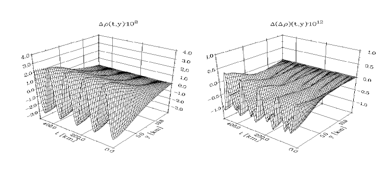
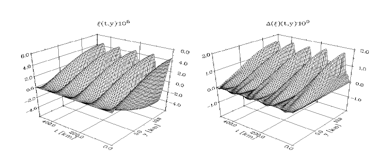
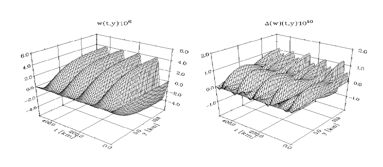
Figure 59: The left panels show the time evolution of $\Delta\rho$, $\xi$ and $w$ obtained for 1600 grid points. The initial perturbation is given as the fundamental mode in the displacement vector $\xi$. The right panels show the deviation from the exact solution of the linearized equations.

exactly. In the remainder of the Lagrangian discussion we will therefore use the relaxation method described in section 5.2.2 to calculate the TOV background. Unless specified otherwise we will use the rescaled coordinate $y$ for this calculation and the time evolution and thus set $r_{,x}=C$.
The next step consists in calculating the eigenmode profiles for the variables $\xi$, $w$ and $\Delta\rho$. These results enable us to specify initial data and calculate the analytic solutions. In this case the initial perturbation of the star consists in a displacement $\xi$ of the fluid elements corresponding to the fundamental mode with a surface amplitude of about $5\,\,{\rm cm}$. The initial velocity is set to zero and the energy density corresponding to this eigenmode follows from Eq. (5.217). The remaining initial variables are calculated from the constraint equations (5.235), (5.236). The resulting data on the initial slice are then evolved in time according to the method described in the previous section. The analytic solution for the fundamental variables $\xi$, $w$, $\Delta\rho$ is given by

$$\xi(t,x) =\xi_{1}(x)\cos{\omega t},$$ (5.245)

$$w(t,x) =-w_{1}(x)\sin{\omega t},$$ (5.246)

$$\Delta\rho =\Delta\rho_{1}(x)\cos{\omega t},$$ (5.247)

where $\omega$ is the frequency derived from the eigenmode calculation. In Fig. 59 we show the numerical results obtained for 1600 grid points together with their deviation from the harmonic solutions. These results show that the code reproduces the analytic solution

Figure 60: Frequency spectra obtained for stellar models with polytropic indices $\gamma=1.75$ (left) and 3.0 (right). The initial data consists of a displacement $\xi$ given by the sum of the first 10 eigenmodes. The vertical bars indicate the frequencies predicted by the eigenmode calculations.

with a relative accuracy of about $10^{-4}$. For presentation purposes the time evolution is shown up to $t=500\,\,{\rm km}$ only. No significant loss of accuracy has been observed for longer evolutions.
We have also compared the frequency spectrum resulting from time evolutions with the corresponding predictions by the eigenmode calculation. For this purpose we have used the same stellar model as in the previous test as well as model 1 of Table 3 which has a polytropic index $\gamma=1.75$. In both cases the initial perturbation is given by the sum of the first ten eigenmodes in the displacement $\xi$. The combined amplitude is about $10\,\,{\rm cm}$ in both cases, so that the deviation from the linear approximation should again be very small. In Fig. 60 we show the Fourier spectra of the central energy density perturbation $\Delta\rho(t,0)$ obtained for time evolutions over $1500\,\,{\rm km}$ using 600 grid points. The vertical bars indicate the frequencies predicted for the first 10 eigenmodes and coincide well with the peaks in the power spectra.
In order to test the performance of the code in the non-linear regime

Figure 61: The convergence factor for $\xi$, $w$, $\Delta N$, $\Delta\rho$ and $\Delta\lambda$ obtained for 400 and 800 grid points. The reference solution has been calculated for 1600 grid points.

we have performed a convergence analysis for an initial displacement with the profile of the second eigenmode and an amplitude of about $50\,\,{\rm m}$ for the stellar model with $\gamma=3$ and $K=2.0\cdot 10^{5}\,\,{\rm km}^{-2}$. In this amplitude range non-linear effects are present, but shock formation is not yet expected for initial data with sufficiently weak spatial variation. We have evolved these initial data using 400, 800 and 1600 grid points and have calculated the time dependent convergence factor according to the method described in section 3.5.3. Since the exact solution is not known, we use the reference solution for 1600 grid points in its place. The result obtained for the variables $\xi$, $w$, $\Delta N$, $\Delta\rho$ and $\Delta\lambda$ is shown in Fig. 61 and demonstrates second order convergence throughout the evolution.
Finally we have tested the code with the analytic solution by Oppenheimer1939b which describes the collapse of a homogeneous spherically symmetric dust cloud. Petrich1986 have expressed this analytic solution in polar slicing combined with radial or isotropic gauge. Even though we are using a Lagrangian gauge condition here, we can use their results for a comparison with our numerical simulation.
In their calculation of the analytic solution Petrich1986 use a Lagrangian coordinate $\chi$ and a time parameter $\eta$ which varies from $-\pi$ to $0$ as the dust sphere collapses from initial radius to $\hat{r}=0$. On a given time slice $t=\mathrm{const}$, where $t$ is the time coordinate defined by the polar slicing condition, $\eta$ is given as a function of $\chi$ by

$$\cos{\frac{\eta}{2}} =\cos{\frac{\eta_{\rm s}}{2}}\sqrt{\frac{\cos{\chi_{\rm s}}}{\cos{\chi}}},$$ (5.248)

where $\eta_{\rm s}$ and $\chi_{\rm s}$ are the values of $\eta$ and $\chi$ at the surface of the dust cloud. If we label the initial slice by $\eta_{\rm s}=-\pi$, this equation implies that $\eta=-\pi$ everywhere on the initial slice. At any given time $t$ the areal radius is then shown to be related to the coordinate $\chi$ by

$$\hat{r} =2M\frac{\sin{\chi}}{\sin^{3}{\chi_{\rm s}}}\left(1-\cos^{2}\frac{\eta_{\rm s}}{2}\cdot\frac{\cos{\chi_{\rm s}}}{\cos{\chi}}\right),$$ (5.249)

where $M$ is the Schwarzschild mass of the dust cloud. If we consider the special case of this equation at the surface and on the initial slice we can calculate $\chi_{\rm s}$ from

$$\sin^{2}{\chi_{\rm s}} =\frac{2M}{R},$$ (5.250)

where $R$ is the initial radius of the dust sphere. For reasons that will be given below we will identify the radial coordinate $x$ with the areal radius of the initial location of the fluid elements. We can therefore set $\eta_{\rm s}=-\pi$ and $\hat{r}=x$ in Eq. (5.249) and use the result to calculate $\chi(x)$ on the initial slice. Since both coordinates are comoving with the fluid elements, this relation between $\chi$ and $x$ remains valid at any time $t$. In order to calculate $\eta(x)$ at a given time $t$ we still need to find the value $\eta_{\rm s}$. This is done by inverting the relation

$$t =M\frac{\cos{\chi_{\rm s}}}{\sin^{3}{\chi_{\rm s}}}\left\{(\eta_{\rm s}-\sin{\eta_{\rm s}})+2\sin^{2}{\chi_{\rm s}}\left[\eta_{\rm s}-2\tan{\chi_{\rm s}}\mathop{\rm tanh}^{-1}\nolimits{\left(\tan{\chi_{\rm s}}\cot{\frac{\eta_{\rm s}}{2}}\right)}\right]\right\},$$ (5.251)

for which we use a Newton-Raphson method. Once $\eta_{\rm s}$ has been calculated, we can use Eq. (5.248) to calculate $\eta(x)$ on that time slice. The physical variables $\hat{r}$, $\hat{\rho}$, $\hat{\Gamma}$ and $\hat{\lambda}$ then follow from Eq. (5.249) and further relations by Petrich1986 which we write in the form

$$\hat{\rho} =6\frac{a_{0}}{a^{3}}\frac{1}{8\pi M^{2}},$$ (5.252)

$$\hat{\Gamma} =\frac{\cos^{3}{\chi}-\cos^{2}{\frac{\eta_{\rm c}}{2}}}{\cos{\chi}-\cos^{2}{\frac{\eta_{\rm c}}{2}}},$$ (5.253)

$$\hat{\lambda} =-\frac{\hat{\lambda}_{\rm c}}{\sin{\frac{\eta_{\rm c}}{2}}}\frac{\cos{\chi}-\cos^{2}{\frac{\eta_{\rm c}}{2}}}{\sqrt{\cos^{3}{\chi}-\cos^{2}{\frac{\eta_{\rm c}}{2}}}},$$ (5.254)

where $\lambda_{\rm c}$ is the central value of the lapse function and $a_{0}$ and $a$ are given by

$$a_{0} =\frac{1}{\sin^{3}{\chi_{\rm s}}},$$ (5.255)

$$a =a_{0}(1-\cos{\eta}).$$ (5.256)

In practice we specify the initial energy density and radius of the dust sphere and set the velocity to zero. The functions $\hat{N}$ and $\hat{\lambda}$ are then calculated from the constraint equations and the total mass of the sphere follows from the definition (5.219).
From the numerical point of view the dust collapse is a special

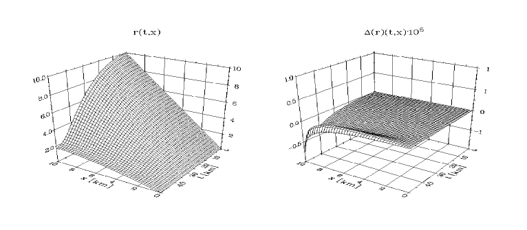
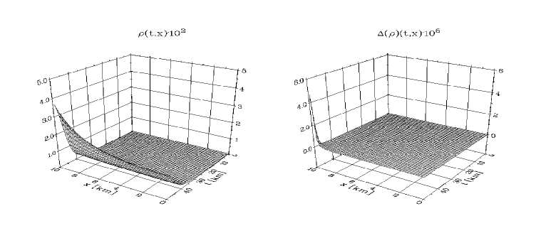
Figure 62: The numerical simulation of the Oppenheimer-Snyder dust collapse for a dust sphere of $10\,\,{\rm km}$ radius and initial density $2\cdot 10^{-4}\,\,{\rm km}^{-2}$. The left panels show the numerical results for the radius $\hat{r}$ and the energy density $\hat{\rho}$, the right panels the deviation from the analytic solution.

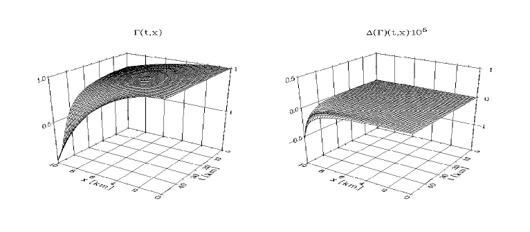
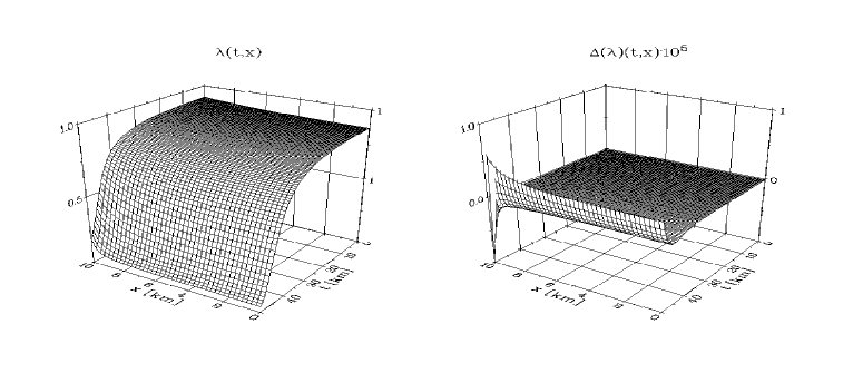
Figure 63: Same as Fig. 62 for the metric variables $\hat{\Gamma}$ and $\hat{\lambda}$.

case in several aspects which restricts our choice of the available options of the code.

• By definition the pressure vanishes in the dust sphere. As a result there is no static configuration analogous to the static neutron star governed by the TOV equations. We therefore need to use vacuum flat space as the background and run the code in the non-perturbative mode.

• The vanishing of the pressure also implies that the speed of sound is zero throughout the dust sphere so that it cannot be used to rescale the radial coordinate according to Eq. (5.47). The radial coordinate $x$ is therefore defined by the areal radius of the initial positions of the fluid elements and we use the condition $r_{,x}=1$ in the code.

• The surface of a neutron star with a polytropic equation of state is defined by the vanishing of the energy density $\hat{\rho}$ which provided the outer boundary condition in the numerical evolution. For the dust sphere this relation is not valid any more and the energy density is finite at the outer boundary. The exact value, however, is not known, so that we cannot use it to derive an alternative boundary condition. The boundary condition $\hat{P}=0$ is trivially satisfied in the case of a dust sphere and does not provide any extra information either. If we consider the structure of equations (5.220)-(5.224), however, we can see that all spatial derivatives of the energy density appear in the form of pressure gradients. These terms are identically zero in this case and disappear from the equations. We can therefore use the staggered grid for the energy density and thus eliminate the need of a boundary condition for $\hat{\rho}$. For this purpose we set the parameter $\sigma$ to 1 in the evolution of the dust sphere.

In Figs. 62 and 63 we show the results obtained for a dust sphere with initial density $\hat{\rho}_{0}=2\cdot 10^{-4}\,\,{\rm km}^{-2}$ and radius $R_{0}=10\,\,{\rm km}$ which corresponds to a total mass of $M=0.838\,\,{\rm km}$. A grid resolution of 800 points has been used for this calculation. The results demonstrate the good accuracy with which the code reproduces the analytic solution. Near the surface of the dust sphere, however, the numerical error increases significantly as the sphere approaches its Schwarzschild radius. We attribute this behaviour to the steep gradient of the lapse function near the surface that arises in the late stages of the evolution.
This simulation also illustrates the singularity avoiding properties of the polar slicing condition. As the dust sphere collapses towards its Schwarzschild radius, the lapse function decreases towards zero and the evolution is practically frozen. This effect, the so called collapse of the lapse, is responsible for the apparent slow down of the collapse of the radial function $r$ that can be seen in the upper left panel of Fig. 62. It is this property that makes polar slicing a popular choice for the numerical analysis of 1-dimensional gravitational collapse.

5.5 Do shocks form at the surface for low amplitude oscillations?

We will now address a question that implicitly arose in the discussion of the linearized equations in the Eulerian formulation. We have seen in Eq. (5.133) that the linearized equations predict a diverging ratio $\delta\rho/\rho$ at the surface. For polytropic indices $\gamma>2$ we know that the divergence of $\delta\rho$ is a result of the Taylor expansion used to relate the Eulerian energy density perturbation to the Lagrangian one in Eq. (5.130) and thus a non-physical result. For polytropic exponents $\gamma\leq 2$, however, Eq. (5.130) represents a valid relation to first order in the perturbations, so that the Eulerian density perturbation will indeed be large compared with the background value near the surface. This behaviour raises the question whether non-linear effects will affect the evolution near the surface and give rise to the formation of discontinuities. From a different point of view one may consider the speed of sound which vanishes at the surface for a polytropic exponent $\gamma>1$ and the particle speed $w$ which is finite because of the movement of the stellar surface. Consequently the velocity of the fluid elements will exceed the speed of sound and one may again ask whether this leads to shock formation. We will investigate this by using the exact treatment of the surface provided by the Lagrangian code.
For this purpose we consider the neutron star model 3 of Table 3 and provide initial data in the form of a displacement $\xi$ corresponding to a single eigenmode. For reasonably low order eigenmodes and amplitudes up to several metres we have not observed any significant deviation from the expected harmonic time dependence. For eigenmodes of very high order, however, this picture changes. We illustrate this in the case of an initial displacement of the fluid elements corresponding to a high order eigenmode (about 50) and an amplitude of about $1\,{\rm m}$ at the surface. The high resolution of 3200 grid points has been used for this calculation to adequately resolve the high order mode. We stress that this evolution is only possible because of the high resolution near the surface provided by the rescaled variable $y$.

Figure 64: The numerical evolution of the energy density perturbation $\Delta\rho$ as a function of $y$ obtained for an initial displacement corresponding to about the 50th eigenmode with amplitude $1\,{\rm m}$. Snapshots are shown at times $t_{1}\ldots,t_{8}$.

In Fig. 64 we show snapshots of the time evolution of the energy density perturbation at times $t_{1}=0.0$, $t_{2}=0.5$, $t_{3}=1.0$, $t_{4}=1.5$, $t_{5}=2.0$, $t_{6}=2.5$, $t_{7}=3.0$ and $t_{8}=3.1\,{\rm km}$. We note that only the small radial range $28\,{\rm km}\leq y\leq 31.7\,{\rm km}$ is shown in the figure. In terms of the areal radius this corresponds to a range of about $120\,{\rm m}$ below the surface. We can see that for this small amplitude a steep gradient forms near the surface after about $t=3.1\,{\rm km}$ which corresponds to less than two oscillation periods of the eigenmode. This indicates the formation of a discontinuity. At later times than shown here the code fails to converge which we attribute to the numerical noise caused by the shock formation and the extreme sensitivity of the code near the surface of the star. In order to demonstrate that this result is not merely due to numerical inaccuracies, we have evolved the same initial data with the smaller amplitude of $1\,{\rm cm}$. In Fig. 65 we show the same snap shots for this evolution as in Fig. 64. In this case we obtain harmonic time dependence as expected in the linear limit.

Figure 65: The same as Fig. 64 but for an amplitude of $1\,{\rm cm}$.

By using eigenmodes with even higher order we have observed shock formation at the surface for smaller amplitudes. In view of the results for low order modes where no significant non-linear effects are observed for similar amplitudes, we conclude that the magnitude of non-linear effects is not only determined by the size of the perturbations relative to the background variables, but also by the length scale on which the perturbations vary significantly. We finally note that the surface of a neutron star is too complicated to be accurately described by the polytropic equation of state used for these evolutions. It is not clear whether discontinuities will form in the same way for more realistic descriptions of neutron stars. Nevertheless our results demonstrate that the surface requires a careful numerical treatment.

6 Conclusions

In this work we have presented the application of different numerical techniques to solve Einstein’s field equations. We have laid the foundation for our discussion by describing in detail the ADM “3+1” and the characteristic Bondi-Sachs formulation of the field equations together with various aspects of numerical analysis.
In the framework of “3+1” formulations of the Einstein field equations the restriction to a finite grid in numerical computations results in difficulties concerning the specification of outer boundary conditions and the interpretation of gravitational waves. These problems are naturally resolved in a characteristic formulation, but the foliation of spacetime based on the characteristic surfaces may break down in regions of strong curvature due to the formation of caustics. The combination of the two schemes in the framework of Cauchy-characteristic matching enables one to make use of the advantages of both methods while avoiding the respective drawbacks. In this work we have completed the cylindrically symmetric stage of the Southampton Cauchy-characteristic matching project by providing a new long term stable CCM code including both gravitational degrees of freedom. A Geroch decomposition of the 4-dimensional spacetime allows us to reformulate the problem in terms of the norm of the axial Killing vector $\nu$ and the Geroch potential $\tau$ on an asymptotically flat 3-dimensional quotient spacetime. These geometrical fields describe the gravitational degrees of freedom in simple terms and appear to be a natural choice of variables for the description of a cylindrically symmetric vacuum spacetime. The conformal compactification of the resulting 3-dimensional spacetime allows us to impose exact boundary conditions at null infinity. In contrast to the previous work we have also applied the Geroch decomposition to the interior Cauchy region and thus been able to use the same variables throughout the numerical grid. This leads to a substantial simplification of the interface and the evolution equations and facilitates a long term stable evolution with both gravitational degrees of freedom present. The effectiveness of the code has been demonstrated by reproducing the analytic Weber-Wheeler solution and the vacuum spacetime with two degrees of freedom due to Xanthopoulos. The code has been shown to be second order convergent over the dynamically relevant time intervals. Our results demonstrate the importance of a “good” choice of variables in order to obtain a stable, accurate code even in the 1-dimensional case. For higher dimensional problems the structure of the null-geodesics will be much more complicated because of the angular dependence. As a consequence the transformation between the Cauchy and the characteristic variables at the interface will also be more complicated and thus more vulnerable to instabilities. In view of our results it seems preferable to search for natural variables, such as the Geroch variables in the cylindrically symmetric case, to describe the two regions rather than follow the “brute force” calculations which arise for example from a direct application of the ADM-formulation in the Cauchy region.

Next we have derived a characteristic formulation of the equations governing a dynamic cosmic string in cylindrical symmetry. A feature of the cosmic string equations is that they admit exponentially diverging unphysical solutions. By using the Geroch decomposition it is again possible to reformulate the problem in terms of fields which describe the string on an asymptotically flat $2+1$-dimensional spacetime and the two auxiliary fields $\nu$ and $\tau$. As well as avoiding the need to introduce artificial outgoing radiation boundary conditions the inclusion of null infinity as part of the numerical grid has the advantage that we can enforce outer boundary conditions for the string variables which rule out the unphysical solutions. As special cases of the dynamic equations we also obtain the equations for a static cosmic string in curved or Minkowski spacetime. These sets of equations have been solved by using a relaxation scheme in the static cases and an implicit method for the dynamic scenario.
A convergence analysis for all codes demonstrates clear second order convergence. The dynamic code has also been shown to reproduce the results of the two exact vacuum solutions by Weber & Wheeler and Xanthopoulos. Finally the dynamic code reproduces the results for the static cosmic string in that initial data corresponding to a static solution do not change significantly when evolved in time. For both the exact vacuum solutions and the static initial data the code shows excellent long term stability.
After demonstrating the reliability of the code we have used it to analyse the interaction between an initially static cosmic string and a Weber-Wheeler type pulse of gravitational radiation. We have found that the gravitational wave excites the string and causes the string variables $X$ and $P$ to oscillate. In terms of unphysical rescaled variables we find that the frequencies of the oscillations are essentially independent of the strength of the coupling between string and gravity described by $\eta$ and of the width and amplitude of the Weber-Wheeler pulse. We have also found that the frequency of $X$ is independent of the relative coupling constant $\alpha$ while that of $P$ is proportional to $\sqrt{\alpha}$. When this result is translated back into the physical units we find that the frequency of the scalar field is proportional to the mass of the scalar field and the frequency of the vector field is proportional to the mass of the vector field as predicted by the linearized theory. This result is confirmed by investigating two further scenarios. Firstly we consider the evolution of static initial data for the string coupled to the gravitational field, but with a Gaussian perturbation to one of the string variables, and secondly we consider the same scenario but in a Minkowskian background with the gravitational field decoupled. In both cases we obtain the same relationship between the frequencies and the mass.
An interesting numerical result arising from the use of an implicit numerical scheme concerns the structure of the interface between the interior and the compactified outer region. In contrast to the rather complicated interpolation techniques that were necessary to transform between the Cauchy and characteristic variables in the explicit vacuum CCM-code, we have been able to “localise” the interface in the implicit scheme by using two grid points for the spatial position $r=1$, one containing the variables of the inner region, one containing those used in the outer region. The interface then merely consists in relating these variables and their derivatives by using their definitions and applying the chain-rule. In our case the resulting relations were trivial and could easily be incorporated into the main evolution algorithm. We attribute this substantial simplification to the simultaneous calculation in implicit schemes of all function values on the new time-slice. In explicit schemes, on the other hand the calculation of the new function values is normally subject to a certain hierarchical order.

In the final part of this work we have presented a new numerical approach which enables us to evolve radial oscillations of neutron stars over a large amplitude range with high accuracy. In radial gauge and polar slicing the dynamic star is described by two constraint equations for the metric and a quasi-linear system of two evolution equations for the matter variables. The crucial step in our approach is to decompose the dynamic variables into static background contributions which are determined by the Tolman-Oppenheimer-Volkoff equations and time dependent perturbations. We have used this decomposition to rewrite the system of equations in a perturbative form. We do, however, keep all terms of higher order in the perturbations and thus obtain a formulation equivalent to the original set of equations. The motivation for our approach is given by the fact that background terms (terms of zero order) are in general present in the dynamic equations. These terms cancel each other analytically by virtue of the background equations. Numerically, however, this is generally satisfied up to a residual numerical error only which will constitute a spurious source term in the evolution of the perturbations and contaminate the numerical results. In order to avoid this effect, we use the background equations to remove all zero order terms from the perturbative equations. We thus ensure that the numerical accuracy is determined by the perturbations instead of the static background.
We have compared the resulting perturbative code with a “standard” non-perturbative method by evolving the fundamental eigenmode of a dynamically stable neutron star using an amplitude of several metres. Whereas the perturbative scheme reproduces the expected harmonic oscillations with high accuracy, the non-perturbative scheme leads to an exponential decay of the central energy density perturbation after a few oscillations which we attribute to the numerical contamination caused by the background terms.
Even though the perturbative code performs well in the linear regime for a wide variety of neutron star models, we have observed a spurious exponential growth of the physical variables in the evolution of marginally stable neutron star models if we truncate the neutron star at a sufficiently large density and thus omit the outer low density layers from the numerical evolution. The need to truncate the neutron star at finite densities arises from the occurrence of negative energy densities near the surface of the star due to numerical inaccuracies. In a purely Eulerian formulation the outer grid boundary does not coincide with the surface of the star in a non-linear evolution. When the star shrinks inside the numerical grid negative energy densities will occur because the numerical evolution is not able to accurately model the vacuum region between the stellar surface and the outer grid boundary. It is interesting to see that the surface represents a problematic area even in the comparatively simple linearized case. For equations of state with an asymptotic behaviour $P\sim\rho^{\gamma}$ and $\gamma>2$ the Eulerian energy density perturbation diverges at the surface of the star. We have shown how this problem arises from the transformation between Lagrangian and Eulerian perturbations and is not present in a Lagrangian formulation.
In order to alleviate the surface problem in the Eulerian case in a simple manner we have used a fixed boundary condition by setting the radial velocity $w=0$ at the outer grid boundary. Furthermore we have truncated the outer layers of the neutron star, so that the resulting model contains $90\,\%$ of the original mass. We have thus demonstrated second order convergence of the code in the non-linear regime and checked the conservation properties of the code in the Cowling approximation. We have finally used the simplified neutron star model to study the coupling between eigenmodes due to non-linear effects. For this purpose we have provided initial data in the form of an isolated eigenmode and quantified the excitation of other modes in terms of the inner product, defined by the self-adjoined eigenvalue problem of the linearized case, between the non-linear data and the eigenmode solutions. The high accuracy of the perturbative scheme enables us to vary the amplitude of the initial data over a wide range corresponding to a maximum displacement of fluid elements between several cm and about $50\,{\rm m}$. For significantly larger amplitudes we observe the formation of steep gradients which makes the accurate measurement of the eigenmode coefficients problematic.
In our study we have provided initial data in the form of either of the first three eigenmodes in the velocity field while the energy density perturbation has been set to zero. We have then measured the maximum coefficients for the first 10 or 15 eigenmodes. Our results clearly show the existence of two distinct regimes. In the weakly non-linear regime with amplitudes up to several metres all eigenmode coefficients increase quadratically with the amplitude. If the order of the initially excited mode is $j$, we have also found that the coupling coefficients in the weakly non-linear regime decrease with increasing order of the eigenmodes starting with mode $2j$. This decrease can be approximated well with an inverse cubic power law. In the moderately non-linear regime we have observed a different behaviour of the modes. An initially present mode $j$ has been found to couple more efficiently to the eigenmodes $n\cdot j$, where $n=2$, 3, 4 and so on. For these modes we can model the resulting eigenmode coefficients with a sum of a quadratic power law and a power law of index $n$ with good accuracy. The remaining eigenmode coefficients also show a steeper increase with amplitude than in the weakly non-linear regime, but the power law contribution with exponent larger than two is generally too small to facilitate an accurate measurement.
Finally we have developed a fully non-linear Lagrangian code for the evolution of spherically symmetric dynamic neutron stars. We have demonstrated how the numerical difficulties encountered in the Eulerian case are resolved in the Lagrangian formulation. The code has been shown to accurately reproduce the analytic solution of the linearized equations for low amplitudes and the analytic solution of Oppenheimer and Snyder describing the collapse of a spherically symmetric homogeneous dust sphere. We have furthermore demonstrated second order convergence of the code. The code has been used to investigate non-linear effects near the stellar surface arising in low amplitude oscillations. Whereas we do not observe a significant deviation from the linear regime for low order eigenmodes and amplitudes of several metres, high order eigenmodes of the order of 50 with amplitudes of $1\,{\rm m}$ lead to the formation of steep gradients near the surface due to non-linear effects. We conclude that the magnitude of non-linear effects is not only determined by the relative size of the perturbations with respect to the background but also on the length scale on which the perturbations vary significantly. The high resolution at the surface required for these evolutions has been obtained by the use of a rescaled radial coordinate which naturally takes into account the vanishing of the speed of sound at the surface and facilitates a formulation of the equations in terms of which the slopes of the characteristics are by and large independent of the position in the star.

Appendix A The finite differencing of the Lagrangian equations

We use an implicit second order in space and time finite differencing scheme for the numerical evolution of the fully non-linear perturbative Lagrangian equations (5.235)-(5.239). The parameter $\sigma$ enables us to use the energy density $\rho$, $\Delta\rho$ on the “normal” grid ($\sigma=0$) or the staggered grid ($\sigma=1$). The staggering, however, affects the energy density only. It is therefore suitable to describe the finite differencing for a general function $f$, $\Delta f$ and the energy density $\rho$, $\Delta\rho$. The function $f$ always represents the background variables $r$, $N$ and $\lambda$. Similarly $\Delta f$ stands for the perturbations $\xi$, $w$, $\Delta N$ and $\Delta\lambda$.
In that notation Eqs. (5.235) and (5.236) are converted into finite differences by using

$$f =\frac{1}{2}\left(f_{k}+f_{k+1}\right),$$ (A.1)

$$\rho =\frac{1}{2}\left[(1+\sigma)\rho_{k}+(1-\sigma)\rho_{k+1}\right],$$ (A.2)

$$\Delta f =\frac{1}{2}\left(\Delta f_{k}^{n+1}+\Delta f_{k+1}^{n+1}\right),$$ (A.3)

$$\Delta\rho =\frac{1}{2}\left[(1+\sigma)\Delta\rho_{k}^{n+1}+(1-\sigma)\Delta\rho_{k+1}^{n+1}\right],$$ (A.4)

$$\Delta f_{,x} =\frac{1}{\Delta x}\left(\Delta f_{k+1}^{n+1}-\Delta f_{k}^{n+1}\right).$$ (A.5)

In order to calculate the derivatives of the background variables we use the TOV equations to express them in terms of undifferentiated variables

$$N_{,x} =-2\frac{N}{r}+4\pi\rho,$$ (A.6)

$$\lambda_{,x} =\frac{\lambda}{\Gamma}\left(N+4\pi rP\right).$$ (A.7)

The remaining auxiliary variables follow from the definitions

$$r_{x} =\left\{\parbox{170.71652pt}{ $1\hskip 34.14322pt{\rm if}\,\,\,x=r$ \\ $C\hskip 31.2982pt{\rm if}\,\,\,x=y$, }\right.$$ (A.8)

$$\Gamma =1-2Nr,$$ (A.9)

$$\Delta\Gamma =-2(\hat{N}\xi+r\Delta N),$$ (A.10)

$$P =K\rho^{\gamma},$$ (A.11)

$$\hat{P} =K\hat{\rho}^{\gamma},$$ (A.12)

$$\Delta P =\hat{P}-P,$$ (A.13)

$$C^{2} =\frac{\partial P}{\partial\rho}=\gamma K\rho^{\gamma-1}.$$ (A.14)

The finite difference expressions used for Eqs. (5.237) and (5.238) are given by

$$f =f_{k+1},$$ (A.15)

$$\rho =\frac{1}{2}\left(\sigma\rho_{k}+(2-\sigma)\rho_{k+1}\right),$$ (A.16)

$$\Delta f =\frac{1}{2}\left(\Delta f^{n+1}_{k+1}+\Delta f^{n}_{k+1}\right),$$ (A.17)

$$\Delta\rho =\frac{1}{4}\left[\sigma(\Delta\rho^{n+1}_{k}+\Delta\rho^{n}_{k})+(2-\sigma)(\Delta\rho^{n+1}_{k+1}+\Delta\rho^{n}_{k+1})\right],$$ (A.18)

$$\Delta f_{,t} =\frac{1}{\Delta t}\left(\Delta f^{n+1}_{k+1}-\Delta f^{n}_{k+1}\right),$$ (A.19)

where the total pressure $\hat{P}$ is defined by Eq. (A.12). Finally we finite difference Eq. (5.239) according to

$$f =\frac{1}{2}\left(f_{k}+f_{k+1}\right),$$ (A.20)

$$\rho =\frac{1}{2}\left[(1+\sigma)\rho_{k}+(1-\sigma)\rho_{k+1}\right],$$ (A.21)

$$\Delta f =\frac{1}{4}\left(\Delta f^{n+1}_{k}+\Delta f^{n}_{k}+\Delta f^{n+1}_{k+1}+\Delta f^{n}_{k+1}\right),$$ (A.22)

$$\Delta f_{,x} =\frac{1}{2\Delta x}\left(\Delta f^{n+1}_{k+1}-\Delta f^{n+1}_{k}+\Delta f^{n}_{k+1}-\Delta f^{n}_{k}\right),$$ (A.23)

$$\Delta f_{,t} =\frac{1}{2\Delta t}\left(\Delta f^{n+1}_{k}-\Delta f^{n}_{k}+\Delta f^{n+1}_{k+1}-\Delta f^{n}_{k+1}\right),$$ (A.24)

$$\Delta\rho_{,x} =\frac{1}{2\Delta x}\left(\Delta\rho^{n+1}_{k+1}-\Delta\rho^{n+1}_{k}+\Delta\rho^{n}_{k+1}-\Delta\rho^{n}_{k}\right),$$ (A.25)

$$\Delta\rho_{,t} =\frac{1}{2\Delta t}\left[(1+\sigma)(\Delta\rho^{n+1}_{k}-\Delta\rho^{n}_{k})+(1-\sigma)(\Delta\rho^{n+1}_{k+1}-\Delta\rho^{n}_{k+1}\right).$$ (A.26)

The auxiliary variables are again defined by Eqs. (A.8)-(A.14). We also use the relations

$$\hat{C}^{2} =\gamma K\hat{\rho}^{\gamma-1},$$ (A.27)

$$\rho_{,x} =\frac{P_{,x}}{C^{2}},$$ (A.28)

$$\Delta P_{,x} =(\hat{C}^{2}-C^{2})\rho_{,x}+\hat{C}^{2}\Delta\rho_{,x},$$ (A.29)

$$\Delta P_{,t} =\hat{C}^{2}\Delta\rho_{,t},$$ (A.30)

$$\frac{\partial\hat{C}^{2}}{\partial\hat{\rho}} =(\gamma-1)\frac{\hat{C}^{2}}{\hat{\rho}}.$$ (A.31)

The last relation is needed for the Newton-Raphson method we use to solve the resulting system of non-linear algebraic equations (cf. section 2.3.5).
These finite difference equations result in $5K-5$ algebraic relations, where $K$ is the total number of grid points. In order to determine the $5K$ variables $\xi_{k}$, $w_{k}$, $\Delta N_{k}$, $\Delta\rho_{k}$ and $\Delta\lambda_{k}$ we also need the 5 boundary conditions (5.240)-(5.244) which we now write as

$$\xi_{1} =0,$$ (A.32)

$$w_{1} =0,$$ (A.33)

$$\Delta N_{1} =0,$$ (A.34)

$$\Delta\rho_{K} =0,$$ (A.35)

$$\hat{\lambda}_{K}-\sqrt{1-2\hat{N}_{K}\hat{r}_{K}} =0.$$ (A.36)

References

- [\citeauthoryearAlcubierre, Brügmann, Pollney, Seidel, and TakanashiAlcubierre et al.2001] Alcubierre, M., B. Brügmann, D. Pollney, E. Seidel, and R. Takanashi (2001). Black Hole Excision for Dynamic Black Holes. AEI-2001-021, gr-qc/0104020.
- [\citeauthoryearAnderson, Choquet-Bruhat, and YorkAnderson et al.1997] Anderson, A., Y. Choquet-Bruhat, and J. W. York, Jr. (1997). Einstein-Bianchi Hyperbolic System for General Relativity. Topol. Methods in Nonlinear Analysis. gr-qc/9710041.
- [\citeauthoryearAnderssonAndersson1998] Andersson, N. (1998). A new class of unstable modes of rotating relativistic stars. ApJ 502, 708–713. gr-qc/9706075.
- [\citeauthoryearAndersson and ComerAndersson and Comer2001] Andersson, N. and G. L. Comer (2001). Slowly rotating relativistic superfluid stars. Class. Quantum Grav. 18, 969–1002.
- [\citeauthoryearArnowitt, Deser, and MisnerArnowitt et al.1962] Arnowitt, R., S. Deser, and C. W. Misner (1962). The dynamics of general relativity. In L. Witten (Ed.), Gravitation an introduction to current research, pp. 227–265. John Wiley, New York.
- [\citeauthoryearBalakrishna, Daues, Seidel, Suen, Tobias, and WangBalakrishna et al.1996] Balakrishna, J., G. Daues, E. Seidel, W.-M. Suen, M. Tobias, and E. Wang (1996). Coordinate conditions in three-dimensional numerical relativity. Class. Quantum Grav. 13, L135–142.
- [\citeauthoryearBardeenBardeen1983] Bardeen, J. M. (1983). Gauge and radiation conditions in numerical relativity. In T. Deruelle, N. & Piran (Ed.), Gravitational radiation, pp. 433–441. North-Holland Publishing Company.
- [\citeauthoryearBardeen and PiranBardeen and Piran1983] Bardeen, J. M. and T. Piran (1983). General relativistic axisymmetric rotating systems: coordinates and equations. Phys. Rep. 96, 205–250.
- [\citeauthoryearBaumgarte and ShapiroBaumgarte and Shapiro1999] Baumgarte, T. W. and S. L. Shapiro (1999). Numerical integration of Einstein’s field equations. Phys. Rev. D 59(024007).
- [\citeauthoryearBirkhoffBirkhoff1923] Birkhoff, G. (1923). Relativity and Modern Physics. Harvard University Press, Cambridge Mass.
- [\citeauthoryearBishopBishop1992] Bishop, N. T. (1992). Some aspects of the characteristic initial value problem. In R. A. d’Inverno (Ed.), Approaches to numerical relativity, pp. 20–33. Cambridge University Press, Cambridge.
- [\citeauthoryearBishop, Gómez, Holvorcem, Matzner, Papadopoulos, and WinicourBishop et al.1996] Bishop, N. T., R. Gómez, P. R. Holvorcem, R. A. Matzner, P. Papadopoulos, and J. Winicour (1996). Cauchy-characteristic matching: A new approach to radiation boundary conditions. Phys. Rev. Lett. 76, 4303–4306.
- [\citeauthoryearBishop, Gómez, Holvorcem, Matzner, Papadopoulos, and WinicourBishop et al.1997] Bishop, N. T., R. Gómez, P. R. Holvorcem, R. A. Matzner, P. Papadopoulos, and J. Winicour (1997). Cauchy-characteristic evolution and wave-forms. J. Comput. Phys. 136, 236.
- [\citeauthoryearBishop, Gómez, Isaacson, Lehner, Szilagyi, and WinicourBishop et al.1998] Bishop, N. T., R. Gómez, R. A. Isaacson, L. Lehner, B. Szilagyi, and J. Winicour (1998). Cauchy-characteristic matching. In B. Bhawal and B. R. Iyer (Eds.), On the Black Hole Trail, pp. 383. Kluwer, Dordrecht.
- [\citeauthoryearBona and MassóBona and Massó1992] Bona, C. and J. Massó (1992). Hyperbolic evolution systems for numerical relativity. Phys. Rev. Lett. 68, 1097–1099.
- [\citeauthoryearBona, Massó, Seidel, and StelaBona et al.1995] Bona, C., J. Massó, E. Seidel, and J. Stela (1995). A New Formalism for Numerical Relativity. Phys. Rev. Lett. 75, 600–603.
- [\citeauthoryearBona, Massó, Seidel, and StelaBona et al.1997] Bona, C., J. Massó, E. Seidel, and J. Stela (1997). First order hyperbolic formalism for numerical relativity. Phys. Rev. D 56, 3405–3415. gr-qc/9709016.
- [\citeauthoryearBondi, van der Burg, and MetznerBondi et al.1962] Bondi, H., M. G. J. van der Burg, and A. W. K. Metzner (1962). Gravitational waves in general relativity VII. Waves from axi-symmetric isolated systems. Proc. Roy. Soc. A 269, 21–52.
- [\citeauthoryearBoriakoffBoriakoff1976] Boriakoff, V. (1976). Pulsar AP 201628: High frequency periodicity in the pulse microstructure. ApJ 208, L43–46.
- [\citeauthoryearBowen and YorkBowen and York1980] Bowen, J. M. and J. W. York, Jr. (1980). Time-asymmetric initial data for black holes and black-hole collisions. Phys. Rev. D 21, 2047–2056.
- [\citeauthoryearChandrasekharChandrasekhar1964a] Chandrasekhar, S. (1964a). Dynamical instability of gaseous masses approaching the Schwarzschild limit in general relativity. Phys. Rev. Letters 12, 114–116.
- [\citeauthoryearChandrasekharChandrasekhar1964b] Chandrasekhar, S. (1964b). The dynamical instability of gaseous masses approaching the Schwarzschild limit in general relativity. ApJ 140, 417–433.
- [\citeauthoryearChandrasekharChandrasekhar1970] Chandrasekhar, S. (1970). Solutions of Two Problems in the Theory of Gravitational Radiation. Phys. Rev. Lett. 24, 611–615.
- [\citeauthoryearClarke and d’InvernoClarke and d’Inverno1994] Clarke, C. J. S. and R. A. d’Inverno (1994). Combining Cauchy and characteristic numerical evolutions in curved coordinates. Class. Quantum Grav. 11, 1463–1468.
- [\citeauthoryearClarke, d’Inverno, and VickersClarke et al.1995] Clarke, C. J. S., R. A. d’Inverno, and J. A. Vickers (1995). Combining Cauchy and characteristic codes. I. The vacuum cylindrically symmetric problem. Phys. Rev. D 52, 6863–6867.
- [\citeauthoryearCoddington and LevinsonCoddington and Levinson1955] Coddington, E. A. and N. I. Levinson (1955). Theory of ordinary differential equations. McGraw-Hill, New York.
- [\citeauthoryearCourant, Friedrichs, and LewyCourant et al.1928] Courant, R., K. O. Friedrichs, and H. Lewy (1928). Über die partiellen Differenzengleichungen der mathematischen Physik. Math. Ann. 100, 32–74.
- [\citeauthoryearCourant, Friedrichs, and LewyCourant et al.1967] Courant, R., K. O. Friedrichs, and H. Lewy (1967). On the partial difference equations of mathematical physics. IBM journal 11, 215–234.
- [\citeauthoryeard’Invernod’Inverno2000] d’Inverno, R. (2000). The Southampton Cauchy-characteristic Matching Project. In Gravitational Waves: A Challenge to Theoretical Astrophysics. ICTP Lecture Notes, Trieste, Italy.
- [\citeauthoryeard’Inverno, Dubal, and Sarkiesd’Inverno et al.2000] d’Inverno, R. A., M. R. Dubal, and E. A. Sarkies (2000). Cauchy-characteristic matching for a family of cylindrical solutions possessing both gravitational degrees of freedom. Classical and Quant. Grav. 17, 3157–3170.
- [\citeauthoryeard’Inverno and Vickersd’Inverno and Vickers1996] d’Inverno, R. A. and J. A. Vickers (1996). Combining Cauchy and characteristic codes III: The interface problem in axial symmetry. Phys. Rev. D 54, 4919–4928.
- [\citeauthoryeard’Inverno and Vickersd’Inverno and Vickers1997] d’Inverno, R. A. and J. A. Vickers (1997). Combining Cauchy and characteristic codes IV: The characteristic field equations in axial symmetry. Phys. Rev. D 56, 772–784.
- [\citeauthoryearDubal, d’Inverno, and ClarkeDubal et al.1995] Dubal, M. R., R. A. d’Inverno, and C. J. S. Clarke (1995). Combining Cauchy and characteristic codes. II. The interface problem for vacuum cylindrical symmetry. Phys. Rev. D 52, 6868–6881.
- [\citeauthoryearFoxFox1962] Fox, L. (1962). Numerical Solution of Ordinary and Partial Differential Equations. Pergamon Press.
- [\citeauthoryearFriedman and IpserFriedman and Ipser1992] Friedman, J. L. and J. R. Ipser (1992). Rapidly Rotating Relativistic Stars. Philos. Trans. R. Soc. London, Ser. A 340, 391–422.
- [\citeauthoryearFriedman and SchutzFriedman and Schutz1978] Friedman, J. L. and B. F. Schutz (1978). ApJ 222, 281.
- [\citeauthoryearFriedrichFriedrich1996] Friedrich, H. (1996). Hyperbolic reductions for Einstein’s equations. Class. Quantum Gravit. 13, 1451–1469.
- [\citeauthoryearGarat and PriceGarat and Price2000] Garat, A. and R. H. Price (2000). Nonexistence of conformally flat slices of the kerr spacetime. Phys. Rev. D 61, 124011. gr-qc/0002013.
- [\citeauthoryearGarfinkleGarfinkle1985] Garfinkle, D. (1985). General relativistic strings. Phys. Rev. D 15, 1323–1329.
- [\citeauthoryearGerochGeroch1970] Geroch, R. (1970). A method for generating solutions of Einstein’s equations. J. Math. Phys. 12, 918–924.
- [\citeauthoryearGlass and LindblomGlass and Lindblom1983] Glass, E. N. and L. Lindblom (1983). The radial oscillations of neutron stars. ApJS 53, 93–103.
- [\citeauthoryearGómez, Laguna, Papadopoulos, and WinicourGómez et al.1996] Gómez, R., P. Laguna, P. Papadopoulos, and J. Winicour (1996). Cauchy-characteristic evolution of Einstein-Klein-Gordon systems. Phys. Rev. D 54, 4719–4727.
- [\citeauthoryearGourgoulhonGourgoulhon1991] Gourgoulhon, E. (1991). Simple equations for general relativistic hydrodynamics in spherical symmetry applied to neutron star collapse. Astron. Astrophys. 252, 651–663.
- [\citeauthoryearGourgoulhon and HaenselGourgoulhon and Haensel1993] Gourgoulhon, E. and P. Haensel (1993). Upper bounds on the neutrino burst from collapse of a neutron star into a black hole. Astron. Astrophys. 271, 287–208.
- [\citeauthoryearGourgoulhon, Haensel, and GondekGourgoulhon et al.1994] Gourgoulhon, E., P. Haensel, and D. Gondek (1994). Maximum mass instability of neutron stars and weak interaction processes in dense matter. Astron. Astrophys. 294, 747–756.
- [\citeauthoryearHarrison, Thorne, Wakano, and WheelerHarrison et al.1965] Harrison, B. K., K. S. Thorne, M. Wakano, and J. A. Wheeler (1965). Gravitation Theory and Gravitational Collapse. Univers. Chicago Press, Chicago.
- [\citeauthoryearHulse and TaylorHulse and Taylor1975] Hulse, R. A. and J. H. Taylor (1975). Discovery of a Pulsar in a Binary System. ApJ 195, L51–55.
- [\citeauthoryearJordan, Ehlers, and KundtJordan et al.1960] Jordan, P., J. Ehlers, and W. Kundt (1960). Abh. Wiss. Mainz. Math. Naturwiss. K1, 2.
- [\citeauthoryearKokkotas and RuoffKokkotas and Ruoff2001] Kokkotas, K. D. and J. Ruoff (2001). Radial oscillations of neutron stars. Astron. Astroph. 366, 565. gr-qc/0011093.
- [\citeauthoryearKompaneetsKompaneets1958] Kompaneets, A. S. (1958). Sov. Phys. JETP 7, 659.
- [\citeauthoryearLaguna-Castillo and MatznerLaguna-Castillo and Matzner1987] Laguna-Castillo, P. and R. A. Matzner (1987). Coupled field solutions for U(1)-gauge cosmic strings. Phys. Rev. D 36(12), 3663–3673.
- [\citeauthoryearLe VequeLe Veque1992] Le Veque, R. J. (1992). Numerical Methods for Conservation Laws (second ed.). Birkhäuser Verlag.
- [\citeauthoryearLichnerowiczLichnerowicz1944] Lichnerowicz, A. (1944). L’integration des équations de la gravitation relativiste et le problème des corps. J. Math. Pures et Appl. 23, 37–63.
- [\citeauthoryearMarderMarder1958] Marder, L. (1958). Gravitational waves in general relativity I. Cylindrical waves. Proc. R. Soc. A 244, 524–537.
- [\citeauthoryearMarronetti and MatznerMarronetti and Matzner2000] Marronetti, P. and R. A. Matzner (2000). Solving the Initial Value Problem of two Black Holes. Phys. Rev. Lett. 85, 5500–5503. gr-qc/0009044.
- [\citeauthoryearMartí, Miralles, Alonso, and IbáñezMartí et al.1988] Martí, J. M., J. A. Miralles, J. D. Alonso, and J. M. Ibáñez (1988). Field theoretical model for nuclear and neutron matter. IV radial oscillations of warm cores in neutron stars. ApJ 329, 780–789.
- [\citeauthoryearMay and WhiteMay and White1966] May, M. M. and R. H. White (1966). Hydrodynamic Calculations of General-Relativistic Collapse. Physical Review 141, 1232–1241.
- [\citeauthoryearMay and WhiteMay and White1967] May, M. M. and R. H. White (1967). Stellar Dynamics and Gravitational Collapse. Methods Comput. Phys. 7, 219–258.
- [\citeauthoryearMigdalMigdal1959] Migdal, A. B. (1959). Nucl. Phys. 13, 655.
- [\citeauthoryearMisner and SharpMisner and Sharp1964] Misner, C. W. and D. H. Sharp (1964). Relativistic Equations for Adiabatic, Spherically Symmetric Gravitational Collapse. Phys. Rev. 136 Nr. 2B, B571–B576.
- [\citeauthoryearMisner, Thorne, and WheelerMisner et al.1973] Misner, C. W., K. S. Thorne, and J. A. Wheeler (1973). Gravitation. W. H. Freeman, New York.
- [\citeauthoryearMusgrave, Pollney, and LakeMusgrave et al.1996] Musgrave, P., D. Pollney, and K. Lake (1996). GRtensorII: A package for General Relativity. Fields Institute Communications 15, 313–318. http://grtensor.phy.queensu.ca.
- [\citeauthoryearÓ Murchadha and YorkÓ Murchadha and York1974] Ó Murchadha, N. and J. W. York, Jr. (1974). Initial-value problem of general relativity. I. General formulation and interpretation. Phys. Rev. D 10, 428–436.
- [\citeauthoryearOppenheimer and SnyderOppenheimer and Snyder1939] Oppenheimer, J. R. and H. Snyder (1939). On Continued Gravitational Contraction. Phys. Rev. 56, 455–459.
- [\citeauthoryearOppenheimer and VolkoffOppenheimer and Volkoff1939] Oppenheimer, J. R. and G. M. Volkoff (1939). On Massive Neutron Cores. Phys. Rev. 55, 374–381.
- [\citeauthoryearPenrosePenrose1963] Penrose, R. (1963). Asymptotic properties of fields and spacetimes. Phys. Rev. Lett. 10, 66–68.
- [\citeauthoryearPetrich, Shapiro, and TeukolskyPetrich et al.1986] Petrich, L. I., S. L. Shapiro, and S. A. Teukolsky (1986). Oppenheimer-Snyder collapse in polar time slicing. Phys. Rev. D 33, 2100–2110.
- [\citeauthoryearPiranPiran1983] Piran, T. (1983). Methods of numerical relativity. In T. Deruelle, N. & Piran (Ed.), Gravitational radiation, pp. 203–256. North-Holland Publishing Company.
- [\citeauthoryearPiraniPirani1965] Pirani, F. A. E. (1965). Introduction to gravitational radiation theory. In A. Trautmann, F. A. E. Pirani, and H. Bondi (Eds.), Lectures on general relativity and gravitation: Brandeis summer institute in theoretical physics, Volume 1, pp. 251–369. Englewood Cliffs, NJ: Prentice Hall, Inc.
- [\citeauthoryearPollneyPollney2000] Pollney, D. (2000). Algebraic and numerical techniques in general relativity. Ph. D. thesis, University of Southampton.
- [\citeauthoryearPress, Flannery, Teukolsky, and VetterlingPress et al.1989] Press, W. H., B. P. Flannery, S. A. Teukolsky, and W. T. Vetterling (1989). Numerical Recipes. Cambridge University Press, Cambridge.
- [\citeauthoryearRichtmyer and MortonRichtmyer and Morton1967] Richtmyer, R. D. and K. W. Morton (1967). Difference methods for initial value problems. Wiley.
- [\citeauthoryearRuoffRuoff2000] Ruoff, J. O. (2000). The Numerical Evolution of Neutron Star Oscillations. Ph. D. thesis, Fakultät für Physik der Eberhard-Karls-Universität zu Tübingen.
- [\citeauthoryearSachsSachs1962] Sachs, R. K. (1962). Gravitational waves in general relativity. Proc. Roy. Soc. A 270, 103–126.
- [\citeauthoryearSchinder, Bludman, and PiranSchinder et al.1988] Schinder, P. J., S. A. Bludman, and T. Piran (1988). General-relativistic implicit hydrodynamics in polar-sliced space-time. Phys. Rev. D 37, 2722–2731.
- [\citeauthoryearSeidel and SuenSeidel and Suen1992] Seidel, E. and W.-M. Suen (1992). Towards a singularity-proof scheme in numerical relativity. Phys. Rev. Lett. 69, 1845–1848.
- [\citeauthoryearSethianSethian1999] Sethian, J. A. (1999). Level Set Methods and Fast Marching Methods. Cambridge University Press. second edition.
- [\citeauthoryearShapiro and TeukolskyShapiro and Teukolsky1983] Shapiro, S. L. and S. A. Teukolsky (1983). Black Holes, White Dwarfs, and Neutron Stars. John Wiley & Sons, Inc.
- [\citeauthoryearShellard and VilenkinShellard and Vilenkin1994] Shellard, E. P. S. and A. Vilenkin (1994). Cosmic Strings and other Topological Defects. Cambridge.
- [\citeauthoryearShibata and NakamuraShibata and Nakamura1995] Shibata, M. and T. Nakamura (1995). Evolution of three-dimensional gravitational waves: Harmonic slicing case. Phys. Rev. D 52, 5428–5444.
- [\citeauthoryearSimmonsSimmons1991] Simmons, G. F. (1991). Differential equations with applications and historical notes. McGraw-Hill, Inc. second edition.
- [\citeauthoryearSjödinSjödin2001] Sjödin, K. R. P. (2001). Cosmic Strings in General Relativity. Ph. D. thesis, University of Southampton.
- [\citeauthoryearSjödin, Sperhake, and VickersSjödin et al.2000] Sjödin, K. R. P., U. Sperhake, and J. A. Vickers (2000). Dynamic Cosmic Strings I. Phys. Rev. D 63, 024011 1–14. gr-qc/0002096.
- [\citeauthoryearSjödin and VickersSjödin and Vickers2001] Sjödin, K. R. P. and J. A. Vickers (2001). The thin string limit of Cosmic Strings coupled to gravity. Submitted to Class. Quantum Grav., gr-qc/018009.
- [\citeauthoryearSmarr and YorkSmarr and York1978] Smarr, L. and J. W. York, Jr. (1978). Kinematical conditions in the construction of spacetime. Phys. Rev. D 17, 2529–2551.
- [\citeauthoryearSperhake, Sjödin, and VickersSperhake et al.2000] Sperhake, U., K. R. P. Sjödin, and J. A. Vickers (2000). Dynamic Cosmic Strings II: Numerical evolution of excited Cosmic Strings. Phys. Rev. D 63, 024012 1–15. gr-qc/0003114.
- [\citeauthoryearStachelStachel1962] Stachel, J. J. (1962). Lie derivatives and the Cauchy problem in the general theory of relativity. Ph. D. thesis, Stevens Institute of Technology, Castle Point.
- [\citeauthoryearTaylor and WeisbergTaylor and Weisberg1989] Taylor, J. H. and J. M. Weisberg (1989). Further experimental tests of relativistic gravity using the binary pulsar PSR 1913+16. ApJ 345, 434–450.
- [\citeauthoryearTeukolskyTeukolsky2000] Teukolsky, S. A. (2000). On the Stability of the Iterated Crank-Nicholson Method in Numerical Relativity. Phys. Rev. D 61, 087501. gr-qc/9909026.
- [\citeauthoryearThornburgThornburg1987] Thornburg, J. (1987). Coordinates and boundary conditions for the general relativistic initial data problem. Class. Quantum Grav. 4, 1119–1131.
- [\citeauthoryearTolmanTolman1939] Tolman, R. C. (1939). Static Solutions of Einstein’s Field Equations for Spheres of Fluid. Phys. Rev. 55, 364–373.
- [\citeauthoryearTurok and BrandenburgerTurok and Brandenburger1986] Turok, N. and R. H. Brandenburger (1986). Cosmic strings and the formation of galaxies and clusters of galaxies. Phys. Rev. D 33, 2175–2181.
- [\citeauthoryearVachaspati and VilenkinVachaspati and Vilenkin1984] Vachaspati, T. and A. Vilenkin (1984). Formation and evolutions of cosmic strings. Phys. Rev. D 30, 2036–2045.
- [\citeauthoryearVan HoolstVan Hoolst1996] Van Hoolst, T. (1996). Effects of nonlinearities on a single oscillation mode of a star. Astron. Astroph. 308, 66–76.
- [\citeauthoryearvan Hornvan Horn1980] van Horn, H. M. (1980). Micropulses, drifting subpulses, and nonradial oscillations of neutron stars. ApJ 236, 899–903.
- [\citeauthoryearVäth and ChanmugamVäth and Chanmugam1992] Väth, H. M. and G. Chanmugam (1992). Radial oscillations of neutron stars and strange stars. Astron. Astroph. 260, 250–254.
- [\citeauthoryearVilenkinVilenkin1981] Vilenkin, A. (1981). Gravitational field of vacuum domain walls and strings. Phys. Rev. D 23, 852–857.
- [\citeauthoryearVilenkin and ShellardVilenkin and Shellard1994] Vilenkin, A. and E. P. S. Shellard (1994). Cosmic strings and other topological defects. Cambridge University Press.
- [\citeauthoryearWeber and WheelerWeber and Wheeler1957] Weber, J. and J. A. Wheeler (1957). Reality of the Cylindrical Gravitational Waves of Einstein and Rosen. Rev. Mod. Phys. 29, 509–515.
- [\citeauthoryearWinicourWinicour2001] Winicour, J. (2001). Characteristic evolution and matching. Living Rev. Relativity 2001-3. [Article in Online Journal] cited on 23 Feb 2001, http://www.livingreviews.org/Articles/Volume4/2001-3winicour.
- [\citeauthoryearXanthopoulosXanthopoulos1986] Xanthopoulos, B. C. (1986). Cylindrical waves and cosmic strings of Petrov type D. Phys. Rev. D 34, 3608–3616.
- [\citeauthoryearYorkYork1979] York, Jr., J. W. (1979). Kinematics and dynamics of general relativity. In L. L. Smarr (Ed.), Sources of gravitational radiation, pp. 83–126. Cambridge University Press, Cambridge.
- [\citeauthoryearYorkYork1983] York, Jr., J. W. (1983). The initial value problem and dynamics. In T. Deruelle, N. & Piran (Ed.), Gravitational radiation, pp. 175–201. North-Holland Publishing Company.
- [\citeauthoryearZel’dovichZel’dovich1980] Zel’dovich, Y. B. (1980). Cosmological fluctuations produced near a singularity. Mon. Not. R. Astron. Soc. 192, 663–667.