Black Hole Relics in String Gravity: Last Stages of Hawking Evaporation

Abstract

The endpoint of black hole evaporation is a very intriguing problem of modern physics. Based on Einstein-dilaton-Gauss-Bonnet four dimensional string gravity model we show that black holes do not disappear and should become relics at the end of the evaporation process. The possibility of experimental detection of such remnant black holes is investigated. If they really exist, these objects could be a considerable part of the non baryonic dark matter in our Universe.

1 Introduction

Theoretical physics faces nowadays a great challenge. There is four dimensional Standard Model on one side (and the additional dimensions are not required to explain experimental data) together with inflationary cosmology based on additional scalar fields [1]. On the other side there is the completely supersymmetrical string/M-theory. Building links between those approaches [2] is a very motivating goal of modern physics which could be achieved by the study of microscopic black holes.

As General Relativity is not renormalizable, its direct standard quantization is impossible. To build a semiclassical gravitational theory, the usual Lagrangian should be generalized, which is possible in different ways. One of them is to study the action expansion in scalar curvature, i.e. higher order curvature corrections. At the level of second order, according to the perturbational approach of string theory, the most natural choice is the 4D curvature invariant Gauss-Bonnet term $S_{GB}=R_{ijkl}R^{ijkl}-4R_{ij}R^{ij}+R^{2}$ [3].

With 4D action, it is not possible to consider only $S_{GB}$ because, being full derivative, it does not contribute to the field equations. It must be connected it with a scalar field $\phi$ to make its contribution dynamical. The following 4D effective action with second order curvature corrections can be built:

$$S = \int d^{4}x\sqrt{-g}\Biggl{[}-R+2\partial_{\mu}\phi\partial^{\mu}\phi+\lambda\xi(\phi)S_{GB}+\ldots\Biggr{]},$$

where $\lambda$ is the string coupling constant. As in cosmology, the most simple generalization of the theory (a single additional scalar field) is not possible because while dealing with spherically symmetric solutions, the “no-hair” theorem restriction must be taken into account.

Treating $\phi$ as a dilatonic field, the coupling function $\xi(\phi)$ is fixed from the first string principles and should be written $\exp(-2\phi)$ [4, 5], which leads to :

$$S = \int d^{4}x\sqrt{-g}\Biggl{[}-R+2\partial_{\mu}\phi\partial^{\mu}\phi+\lambda e^{-2\phi}S_{GB}+\ldots\Biggr{]}.$$ (1)

Such type of actions can be considered as one of the possible middle steps between General Relativity and Quantum Gravity. In this paper, we show that this effective string gravity model and its solutions can be applied for a description of the last stages of primordial black holes (PBH) evaporation [8, 9] and suggests possible dark matter candidates [10]. This should be understood in the general framework of Gauss-Bonnet black hole (BH) theory [6, 7].

The paper is organized as follows: In Section II we briefly recall previously obtained results and point out some new features important for this study, Section III is devoted to the establishment of the new Hawking evaporation law (especially for the detailed description of last stages of Gauss-Bonnet BH evaporation), in Section IV we show that the direct experimental registration of such PBHs is impossible, Section V is devoted to PBH relics as dark matter candidates and Section VI contains discussions and conclusions.

2 Black hole minimal mass

2.1 Black hole minimal mass in pure EDGB model

For the sake of completeness, main results from Ref. [7] are briefly repeated.

Starting from the action (1), a static, spherically symmetric, asymptotically flat black hole solution is considered. One of the most convenient choice of metric in this model is

$$ds^{2}=\Delta dt^{2}-\frac{\sigma^{2}}{\Delta}dr^{2}-r^{2}(d\theta^{2}+\sin^{2}\theta d\varphi^{2}),$$ (2)

where $\Delta=\Delta(r)$, $\sigma=\sigma(r)$.

Asymptotic expansion of the solution has the usual quasi-Schwarzschild form,

$$\Delta(r\rightarrow\infty) = 1-\frac{2M}{r}+O\biggl{(}\frac{1}{r}\biggr{)},$$

$$\sigma(r\rightarrow\infty) = 1-\frac{1}{2}\frac{D^{2}}{r^{2}}+O\biggl{(}\frac{1}{r^{2}}\biggr{)},$$

$$\phi(r\rightarrow\infty) = \frac{D}{r}+O\biggl{(}\frac{1}{r}\biggr{)},$$

where $M$ and $D$ are ADM (Arnowit-Dieser-Misner) mass and dilatonic charge respectively. Using a dedicated code, a BH type solution was obtained. This solution provides a regular horizon of quasi-Schwarzschild type and the asymptotic behaviour near this horizon $r_{h}$ is:

$$\Delta = d_{1}(r-r_{h})+d_{2}(r-r_{h})^{2}+\ldots,$$

$$\sigma = s_{0}+s_{1}(r-r_{h})+\ldots,$$

$$\phi = \phi_{00}+\phi_{1}(r-r_{h})+\phi_{2}(r-r_{h})^{2}+\ldots,$$ (3)

where $(r-r_{h})\ll 1$, $s_{0}$, $\phi_{0}=e^{-2\phi_{00}}$ and $r_{h}$ are free independent parameters.

After solving the equations to the first perturbation order, the following limit on the minimal BH size can be obtained:

$$r_{h}^{inf}=\sqrt{\lambda}\ \sqrt{4\sqrt{6}}\phi_{h}(\phi_{\infty}),$$ (4)

where $\lambda$ is a combination of the string coupling constants (fundamental value) and $\phi_{h}(\phi_{\infty})$ is dilatonic value at $r_{h}$, depending upon dilatonic value at infinity which cannot be determined only in the framework of this model. According to this formula and taking into account the numerical values, the minimal BH mass has the order of Planck one (more precisely $\approx 1.8$ Planck masses [7]).

It is necessary to point out that the stability of the solution under time perturbations at the event horizon was described in [11] and was studied at the singularity $r_{s}$ in [12].

Contribution of higher order curvature corrections was studied in [7, 16] to show that, in the bosonic case with heterotic string models (the question is still open in SUSY II), all the new topological configurations are located inside the determinant singularity and, therefore, do not produce any new physical consequences. Our conclusions remain valid when the next higher order curvature corrections are made of pure products of Riemannian tensors. This topic is under additional investigation now.

Gathering these results, it can be concluded that the solution is stable in all the particular points, and, therefore, at all the values of initial data set.

2.2 Effects of moduli fields

Generalizing the model by taking into account the effective contribution of additional compact dimensions in the most simple form — scalar field — the action must be given as

$$S = \int d^{4}x\sqrt{-g}\Biggl{[}-R+2\partial_{\mu}\phi\partial^{\mu}\phi+2\partial_{\mu}\psi\partial^{\mu}\psi+\Biggl{(}\lambda_{\phi}e^{-2\phi}+\lambda_{\psi}\xi(\psi)\Biggr{)}S_{GB}$$ (5)

$$+ \mbox{ higher order curvature corrections}\Biggr{]}.$$

This model was studied into the details in [13]. For current investigations it should be emphasized that when the contribution of moduli field value is considered, a naked singularity can appear if the size of additional dimensions is greater than the BH size. The minimal BH mass must therefore be increased to 10 Planck masses (to avoid being in naked singularity region). It is a key feature because it allows to move away from the Planck region and to use semiclassical approach. If these additional dimensions were non-compact [14] the BH minimal mass would be much greater.

3 Black hole evaporation law

3.1 Probability of transition to the last stage

According to the analysis given in Ref. [18], the transition from prelast to last stage of BH evaporation is forbidden and evaporating PBHs will never reach the minimal mass state. The shape of the BH mass loss rate law changes and becomes the one presented in Fig.2, analogously to the simplified “toy model” presented in [18]. Different types of similar models for BH evaporation were studied in Lovelock gravity [19], string inspired curvature expansions [20] and in many other theories. The numerical values of Gauss-Bonnet BH (important for experimental search analysis) will be presented in section D.

3.2 Approximation to metric functions

In the WKB approximation of the Hawking evaporation process, everything happens in the neighbourhood of the event horizon. As our metric functions $\Delta$ and $\sigma$ depend upon radial coordinate $r$ and black hole mass $M$, i.e. $\Delta=\Delta(M,r)$ and $\sigma=\sigma(M,r)$ (other variables are not important), we can use expansions (2.1), taking into account only the first terms (partially neglecting the dependence upon radial coordinate $r$). Using 2.1, the metric can be written as:

$$\Delta(M,r) = 1-\frac{2M}{r}\epsilon(M)=\frac{1}{2M\epsilon}(r-2M\epsilon(M)),$$

$$\sigma(M,r) = \sigma_{0}(M).$$ (6)

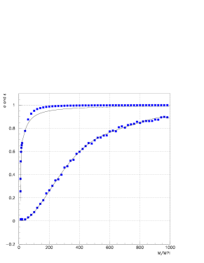
Figure 3: Metric function $\sigma$ and $\epsilon$ as a function of the mass $M$ in Planck units for a fixed minimal mass $M_{Min}=10M_{Pl}$. Stars are numerically computed values and the line is the fit used to derive the spectrum.

Using the numerically calculated data, fits were performed for $\epsilon(M)$ and $\sigma_{0}(M)$. As we are interested mostly in the last stages of PBHs evaporation, where the difference from the standard Bekenstein-Hawking picture is considerable, Taylor expansions around $M_{min}$ can be used. This also helps in obtaining good fits of the metric functions (see Fig.3 and Fig.4) which can be considered as polynom expansions (of $M$ or $1/M$) that are valid between $M=M_{min}=10\ M_{Pl}$ and $M=1000\ M_{Pl}$ with good accuracy.

$$\epsilon = 1-\frac{\epsilon_{1}}{M}-\frac{\epsilon_{2}}{M^{2}}+\frac{\epsilon_{3}}{M^{3}}-\frac{\epsilon_{4}}{M^{4}},$$ (7)

$$\sigma_{0} = \sigma_{2}(M-M_{min})^{2}-\sigma_{3}(M-M_{min})^{3}+\sigma_{4}(M-M_{min})^{4}-\sigma_{5}(M-M_{min})^{5},$$

where (for $M_{min}=10\ M_{Pl}$) the corresponding coefficients are $\epsilon_{1}=10.004$, $\epsilon_{2}=13.924$, $\epsilon_{3}=2856.3$, $\epsilon_{4}=25375.0$, $\sigma_{2}=0.11933*10^{-04}$, $\sigma_{3}=0.30873*10^{-07}$, $\sigma_{4}=0.30871*10^{-10}$, $\sigma_{5}=0.11051*10^{-13}$.

Using this technique, the PBH evaporation spectra and mass loss rate were derived in an analytical form (valid only near the $M_{min}$ point).

3.3 Black hole evaporation spectra in EDGB model

In some approaches, black holes are treated as immersed in a thermal bath and the evaporation can be described as a WKB approximation of semiclassical tunnelling in a dynamical geometry. In our investigation, we follow the techniques described in [21] and [22]. The same method was also applied in [23]. Some other descriptions of BH evaporation can be found in [24, 25].

The key idea of the method from Ref.[21] and [22] is that the energy of a particle changes its sign when crossing the BH horizon. So, a pair created just inside or just outside the horizon can become real with zero total energy after one member of the pair has tunnelled to the opposite side. The energy conservation plays a fundamental role: transitions between states with the same total energy are the only possible ones. Using quantum mechanical rules, it is possible to write the imaginary part of the action for an outgoing positive energy particle which crosses the horizon outwards from $r_{in}$ to $r_{out}$ as:

$$Im(S)=Im\int_{M}^{M-\omega}\int_{r_{in}}^{r_{out}}\frac{dr}{\dot{r}}dH,$$

where $\omega$ is the energy of the particle, $H$ is total Hamiltonian (and total energy) and the metric is written so as to avoid the horizon coordinate singularity. Following [22], Painleve’s coordinates are used. The transformation to this metric from the Schwarzschild one can be obtained by changing the time variable:

$$t=t_{old}+r\sqrt{\frac{\sigma^{2}}{\Delta^{2}}-\frac{1}{\Delta}}.$$

Substituting $t_{old}$ into (2) one obtains

$$ds^{2} = -\Delta dt^{2}+2\sqrt{\sigma^{2}-\Delta}drdt+dr^{2}+r^{2}d\Omega^{2}.$$ (8)

In WKB approximation, the imaginary part of the semiclassical action $Im(S)$, describing the probability of tunnelling through the horizon is

$$Im(S)=Im\int\limits_{r_{in}}^{r_{out}}p_{r}\,dr=Im\int\limits_{r_{in}}^{r_{out}}\int\limits_{0}^{p_{r}}p_{r}^{\prime}\,dr,$$ (9)

where $p_{r}$ is canonical momentum.

For Gauss-Bonnet BH the radial geodesics are described by the equation [7]

$$\dot{r}=\frac{dr}{d\tau}=\frac{\Delta}{\sqrt{\sigma^{2}-\Delta}\mp\sigma}=\mp\sigma-\sqrt{\sigma^{2}-\Delta}.$$ (10)

After substituting expression (10) to the equation (9) one obtains:

$$Im(S) = Im\int\limits_{M}^{M-\omega}\int\limits_{r_{in}}^{r_{out}}\frac{dr}{\dot{r}}dH=-Im\int\limits_{0}^{\omega}\int\limits_{2M\epsilon}^{2(M-\omega)\epsilon}\frac{drd\omega^{\prime}}{\sigma-\sqrt{\sigma^{2}-\Delta}}.$$ (11)

Substituting the expression (3.2) extended in (7) to the equation (11), the imaginary part of the action can be written as:

$$Im(S) = -Im\int\limits_{0}^{\omega}d\omega^{\prime}\Biggl{(}\int\limits_{2M\epsilon}^{2(M-\omega^{\prime})\epsilon}\frac{dr}{\sigma-\sqrt{\sigma^{2}-\frac{r}{2(M-\omega^{\prime})\epsilon}+1}}\Biggr{)}$$

Changing variables with

$$y=\sqrt{\sigma^{2}-\frac{r}{2(M-\omega)\epsilon}+1}.$$

$Im(S)$ takes the form

$$Im(S) = -Im\int\limits_{0}^{\omega}d\omega^{\prime}\Biggl{(}\int\limits_{\sqrt{\sigma^{2}-\frac{\omega^{\prime}}{M-\omega^{\prime}}}}^{\sigma}\frac{4(M-\omega^{\prime})\epsilon ydy}{y-\sigma}\Biggr{)}$$

$$= -Im\int\limits_{0}^{\omega}d\omega^{\prime}\Biggl{(}4(M-\omega^{\prime})\epsilon\sigma\int\limits_{\sqrt{\sigma^{2}-\frac{\omega^{\prime}}{M-\omega^{\prime}}}}^{\sigma}\frac{dy}{y-\sigma}\Biggr{)}$$

$$= -\int\limits_{0}^{\omega}d\omega^{\prime}\left(4(M-\omega^{\prime})\epsilon\sigma\pi\right).$$

As a result the imaginary part of the action is :

$$2Im(S)=\frac{840\pi}{M^{2}(M-\omega)^{2}}\alpha,$$

where $\alpha$ is a huge expression that cannot be written here. It can be found at http://isnwww.in2p3.fr/ams/ImS.ps.

Using the numerical values for a realistic order of $M_{min}$ around 10 Planck masses, the corresponding $\epsilon_{i},$ and $\sigma_{j}$, it is possible to find from (3.2) the approximate expression for $Im(S)$. As we are interested mostly in the last stages of BH evaporation where the influence of higher order curvature corrections is important, the limit $M-M_{min}\ll 1$ can be taken in the computations, leading to a very different spectrum than the standard Bekenstein-Hawking picture (where $-dM/dt\propto 1/M^{2}$). Taking into account energy conservation, $\omega$ can be bounded : $0\leq\omega\leq M-M_{min}$. The approximate expression of $Im(S)(M,\omega)$ for a given $M_{min}$ can then be used in the form

$$Im(S)=k*(M-M_{min})^{3},$$ (12)

where constant $k=5\cdot 10^{-4}$ in Planck unit values with a satisfying accuracy (the plot of $Im(S)$ and its approximation are shown on Fig.5).

3.4 Energy conservation and mass lost rate

Following Ref.[22], the emission spectrum per degree of freedom can simply be written as:

$$\frac{d^{2}N}{dEdt}=\frac{\Gamma_{s}}{2\pi\hbar}\cdot\frac{\Theta((M-M_{min})c^{2}-E)}{e^{Im(S)}-(-1)^{2s}},$$ (13)

$\Gamma_{s}(M,E)$ being the absorption probability for a particle of spin $s$ and the Heavyside function being implemented to take into account energy conservation with a minimal mass $M_{min}$. In this section and in the following ones, standard units are used instead of Planck ones as numerical results should be obtained for experimental fluxes. At this point, two questions have to be addressed: which kind of fields are emitted (and which correlative $\Gamma_{s}$ have to be used) and which mass range is physically interesting. To answer those questions, the mass loss rate is needed:

$$-\frac{dM}{dt}=\int_{0}^{(M-M_{min})c^{2}}\frac{d^{2}N}{dEdt}\cdot\frac{E}{c^{2}}dE$$ (14)

where the integration is carried out up to $(M-M_{min})c^{2}$ so as to ensure that the transition below $M_{min}$ is forbidden. The absorption probabilities can clearly be taken is the limit $GME/\hbar c^{3}\ll 1$ as we are considering the endpoint emission when the cutoff imposed by $M_{min}$ prevents the black hole from emitting particle with energies of the order of $kT$. Using analytical formulae [27] and expanding $\exp(Im(S))$ to the first order with the approximation according to (12), it is easy to show that the emission of spin-1 particles, given by (per degree of freedom)

$$-\frac{dM}{dt}\approx\frac{16}{9\pi}\frac{G^{4}M_{Pl}}{\hbar^{5}c^{2}k}M^{4}(M-M_{min})^{3}$$ (15)

dominates over s=1/2 and s=2 emission whatever the considered energy in the previously quoted limit. It is interesting to point out that the fermion emission around $M_{min}$ is not strongly modified by the EDGB model as, in the lowest order, $\exp(Im(S))-(-1)^{2s}\approx 2$. Furthermore, if energy conservation was implemented as a simple cutoff in the Hawking spectrum, the opposite result would be obtained: s=1/2 particles would dominate the mass loss rate as the power of $(ME)$ in the absorption probability is the smallest one. If we restrict ourselves to massless particles, i.e. the only ones emitted when $M$ is very close to $M_{min}$, the metric modification changes the endpoint emission nature from neutrinos to photons. The real mass loss rate is just twice the one given here to account for the electromagnetic helicity states.

With this expression $-dM/dt=f(M)$, it is possible to compute the mass $M$ at any given time $t$ after formation at mass $M_{init}$ as:

$$t=\int_{M}^{M_{init}}\frac{dM}{f(M)}\approx\frac{9\pi k\hbar^{5}c^{2}}{32G^{4}M_{Pl}^{3}}\times\frac{1}{M_{min}^{4}(M-M_{min})^{2}}$$ (16)

where only the dominant term in the limit $t\rightarrow\infty$ is taken from the analytical primitive of the function. As expected, the result does not depend on $M_{init}$ which is due to the fact that the time needed to go from $M_{init}$ to a few times $M_{min}$ is much less than the time taken to go from a few times $M_{min}$ to $M$ as long as $M_{init}<<10^{15}~{}{\rm g}$ for $t\approx 10^{17}~{}{\rm s}$. At time $t$ after formation, the mass is given by:

$$M\approx M_{min}+\sqrt{\frac{9k\pi\hbar^{5}c^{2}}{8M_{min}^{4}G^{4}M_{Pl}^{3}t}}$$ (17)

This mass can be implemented in the emission spectrum formula:

$$\frac{d^{2}N}{dEdt}\approx\frac{32}{3\pi}\left(\frac{8}{9\pi}\right)^{\frac{3}{2}}G^{10}\hbar^{-\frac{25}{2}}c^{-15}M_{Pl}^{\frac{15}{2}}M_{min}^{10}$$

$$k^{-\frac{5}{2}}\times t^{\frac{3}{2}}E^{4}\Theta\left(\sqrt{\frac{9k\pi\hbar^{5}c^{6}}{8M_{min}^{4}G^{4}M_{Pl}^{3}t}}-E\right)$$ (18)

leading to a frequency f given by

$$f=\int_{0}^{(M-M_{min})c^{2}}\frac{d^{2}N}{dEdt}dE\approx\frac{36}{15}\cdot\frac{1}{t}.$$ (19)

If we want to investigate the possible relic emission produced now from PBHs formed in the early universe with small masses, this leads to a frequency around $6\cdot 10^{-18}~{}{\rm Hz}$ with a typical energy of the order of $1.8\cdot 10^{-6}$ eV. This emission rate is very small as it corresponds to the evaporation into photons with wavelength much bigger that the radius of the black hole. It should, nevertheless, be emphasized that the spectrum is a monophonically increasing function of energy, up to the cutoff, with a $E^{4}$ behaviour. Furthermore, it shows that, although very small in intensity, the evaporation never stops and leads to a mass evolution in $1/\sqrt{t}$.

4 Experimental detection

We investigate in this section the possibility to measure the previously given relic emission. Let $R$ be the distance from the observer, $z$ the redshift corresponding to the distance $R$, $\theta$ the opening angle of the detector (chosen so that the corresponding solid angle is $\Omega=1~{}sr$), $d^{2}N/dEdt(E,t)$ the individual differential spectrum of a black hole relic (BHR) at time $t$, $\rho(R)$ the numerical BHR density taking into account the cosmic scale factor variations, $R_{max}$ the horizon in the considered energy range, $t_{univ}$ the age of the Universe and $H$ the Hubble parameter. The ”experimental” spectrum $F$ (J${}^{-1}\cdot$s${}^{-1}\cdot$sr^-1) can be written as:

$$F=\int_{0}^{Rmax}\frac{d^{2}N}{dEdt}\left(E(1+z),t_{univ}-\frac{R}{c}\right)$$

$$\times\frac{\rho(R)\cdot\pi R^{2}tan^{2}(\theta)}{4\pi R^{2}}{\rm d}R$$ (20)

which leads to:

$$F=\cdot tan^{2}(\theta)\frac{8}{3\pi}\left(\frac{8}{9\pi}\right)^{\frac{3}{2}}G^{10}\hbar^{-\frac{25}{2}}c^{-15}M_{Pl}^{\frac{15}{2}}M_{min}^{10}$$

$$\times k^{-\frac{5}{2}}E^{4}\int_{0}^{R_{max}}\rho(R)\left(\frac{1+\frac{HR}{c}}{1-\frac{HR}{c}}\right)^{2}(t_{univ}-\frac{R}{c})^{\frac{3}{2}}$$

$$\times\Theta\left(\sqrt{\frac{9k\pi\hbar^{5}c^{6}}{8M_{min}^{4}G^{4}M_{Pl}^{3}(t-\frac{R}{c})}}-E\sqrt{\frac{1+\frac{HR}{c}}{1-\frac{HR}{c}}}\right){\rm d}R$$

This integral can be analytically computed and takes into account both the facts that BHRs far away from Earth must be taken at an earlier stage of their evolution and that energies must be redshifted. Even assuming the highest possible density of BHRs ($\Omega_{BHR}=\Omega_{CDM}\approx 0.3$) and $R_{max}$ around the Universe radius, the resulting flux is extremely small: $F\approx 1.1\cdot 10^{7}~{}{\rm J}^{-1}~{}{\rm s}^{-1}~{}{\rm m}^{-2}~{}{\rm sr}^{-1}$ around $10^{-6}$ eV, nearly 20 orders of magnitude below the background. This closes the question about possible direct detection of BHRs emission.

Another way to investigate differences between EDGB black holes particle emission and a pure Hawking spectrum is to study the mass region where $dM/dt$ is maximal. Taking into account that the mass loss rate becomes much higher in the EDGB case than in the usual Hawking picture, it could have been expected that the extremely high energy flux was strongly enhanced. In particular, it could revive the interest in PBHs as candidates to solve the enigma of measured cosmic rays above the GZK cutoff. Nevertheless, the spectrum modification becomes important only when the mass is quite near to $M_{min}$. Depending on the real numerical value of $M_{min}$, it can vary substantially (increasing with increasing $M_{min}$) but remains a few Planck masses above $M_{min}$. This is far too small to account for a sizeable increase of the flux. The number of particles emitted above $10^{20}$eV in a pure Hawking model is of the order of $10^{15}$ [9]. This value should be taken with care as it relies on the use of leading log QCD computations of fragmentation functions far beyond the energies reached by colliders but the order of magnitude is correct. On the other hand, even if all the energy available when EDGB modifications becomes important were released in $10^{20}$ eV particles (which is not realistic) it would generate only a few times $10^{9}$ particles and modify by less than 0.01% the pure Hawking flux. It would not allow to generate, as expected, a spectrum harder than $E^{-3}$.

5 Primordial black holes as dark matter candidates

The idea of PBH relics as a serious candidate for cold dark matter was first mentioned in [10]. It was shown that in a Friedman universe without inflation, Planck-mass remnants of evaporating primordial black holes could be expected to have close to the critical density. Nevertheless, the study was based on the undemonstrated assumption that either a stable object forms with a mass around $M_{Pl}$ or a naked space-time singularity is left. Our study provides new arguments favouring massive relic objects, probably one order of magnitude above Planck mass and could revive the interest in such non-baryonic dark matter candidates. An important problem is still to be addressed in standard inflationary cosmology: the rather large size of the horizon at the end of inflation. The standard formation mechanism of PBHs requires the mass of the black holes to be of the order of the horizon mass at the formation time and only those created after inflation should be taken into account as the huge increase of the scale factor would extremely dilute all the ones possibly formed before. It is easy to show that under such assumptions the density of Planck relics is very small:

$$\Omega_{Pl}=\Omega_{PBH}\frac{\alpha-2}{\alpha-1}M_{H}^{1-\alpha}M_{*}^{\alpha-2}M_{min}$$ (22)

where $\Omega_{PBH}$ is the density of PBHs not yet evaporated, $\alpha$ is the spectral index of the initial mass spectrum (=5/2 in the standard model for a radiation dominated Universe), $M_{*}$ is the initial mass of a PBH which evaporating time is the age of the Universe ($\approx 5\cdot 10^{14}$g) and $M_{H}$ is the horizon mass at the end of inflation. This latter can be expressed as

$$M_{H}=\gamma^{\frac{1}{2}}\frac{1}{8}\frac{M_{Pl}}{t_{Pl}}t_{i}\approx\gamma^{\frac{1}{2}}\frac{1}{8}\frac{M_{Pl}}{t_{Pl}}\frac{0.24}{(T_{RH}/1{\rm Mev})^{2}}$$ (23)

where $T_{i}$ is the formation time and $T_{RH}$ is the reheating temperature. Even with the highest possible value for $T_{RH}$, around $10^{12}$ GeV (according to Ref. [28] if the reheating temperature is more than $10^{9}$ GeV, BHR remnants should be present nowadays) and the upper limit on $\Omega_{PBH}$ coming from gamma-rays, around $6\cdot 10^{-9}$ the resulting density is extremely small: $\Omega_{Pl}\approx 10^{-16}$.

There are, nevertheless, at least two different ways to revive the interest in PBH dark matter. The first one is related to relics that would be produced from an initial mass spectrum decreasing fast enough, so as to overcome the gamma-rays limit. The second one would be to have a large amount of big PBHs, between $10^{15}$g and $10^{25}$g, where experiments are completely blind: such black holes are too heavy to undergo Hawking evaporation and too light to be seen by microlensing experiments (mostly because of the finite size effect [29]). The most natural way to produce spectra with such features is inflationary models with a scale, either corresponding to a change in the spectral index of the fluctuations power spectrum [30] either corresponding to a step [31].

6 Discussion and conclusions

In this paper, the BH type solution of 4D effective string gravity action with higher order curvature corrections was applied to the description of BHRs. A corrected version of the evaporation law near the minimal BH mass was established. It was shown that the standard Bekenstein-Hawking evaporation forluma must be modified in the neighbourhood of the last stages. Our main conclusion is to show that contrarily to what is usually thought the evaporation does not end up by the emission of a few quanta with energy around Planck values but goes asymptotically to zero with an infinite characteristic time scale.

The direct experimental registration of the products of evaporation of BHRs is impossible. This gives an opportunity to consider these BHRs as one of the main candidates for cold dark matter in our Universe.

Figure 1: Illustration of the moment of last transition. Prelast state is characterized by the regular horizon with the usual quasi-Schwarzschild configuration. The last state is singular configuration making the transition from prelast to last state forbidden.

Figure 2: Shape of BH mass lost rate versus BH mass in Gauss-Bonnet case when the energy conservation is taken into account. Right part of the graph represents the usual Hawking evaporation law when $-dM/dt\sim 1/M^{2}$. Left part shows the picture at last stages when evaporation decelerates and then stops, distinguishing the minimal possible mass (“ground state”).

Figure 4: $Im(S)$ (dots) and the fit $(5\cdot 10^{-4})*(M-M_{min})^{3}$ (dashed line) versus BH mass $M$ during the last stages of BH evaporation in the Gauss-Bonnet case with $M_{min}=10.6M_{Pl}$. It is necessary to note that during last stages of evaporation the emitted energy $\omega<M-M_{min}\ll 1$. For fixed values of $\omega=\omega^{*}_{i}$ in the vicinity of $M_{min}$ ($O(M_{min})=0.01$) the mass $M\in(M_{min}+\omega^{*}_{i},M_{min}+\omega^{*}_{i}+O(M_{min}))$. So, for different values of $\omega^{*}$ ($\omega^{*}_{i+1}=\omega^{*}_{i}+O(M_{min}),\omega^{*}_{1}=0.1,i\in N$) $M$ belongs to different (without intersection) intervals. Finally, $Im(S)$ is represented as connection of such intervals with the most probable values of $\omega^{*}_{i}\in(0.1,1.1)$.

References

- [1] A. Linde, Phys.Rept, 333, 575 (2000).
- [2] S.W.Hawking, Phys.Rev. D62, 043501 (2000).
- [3] C.G.Callan, D.Friedan, E.J.Martinec, N.J.Pery, Nucl. Phys. B294, 593 (1985).
- [4] A.Tseytlin, “String Solutions with Nonconstant Scalar Fields” Published in the proceedings of International Symposium on Particle Theory, Wendisch-Rietz, Germany, 7-11 Sep 1993 (Ahrenshoop Symp.1993:0001-13), hep-th/9402082
- [5] B.Zwiebach, Phys.Lett. B156, 315 (1985); E.Poisson, Class.Quant.Grav. 8, 639 (1991); D.Witt, Phys.Rev. D38, 3000 (1988); J.T.Wheeler, Nucl.Phys. B268, 737 (1986), Nucl.Phys. B273, 732 (1986); G.W.Gibbons and K.Maeda, Nucl.Phys. B298, 741 (1988); D.Garfincle, G.Horowitz and A.Strominger, Phys.Rev. D43, 3140 (1991), Phys.Rev. D45, 3888 (1992).
- [6] S. Mignemi and N.R. Stewart, Phys. Rev. D47, 5259 (1993); P. Kanti, N.E. Mavromatos, J. Rizos, K. Tamvakis and E. Winstanley, Phys. Rev. D54, 5049 (1996); T. Torii, H. Yajima, and K. Maeda, Phys. Rev. D55, 739 (1997).
- [7] S.O. Alexeyev and M.V. Pomazanov, Phys. Rev. D55, 2110 (1997); S.O. Alexeyev and M.V. Sazhin, Gen. Relativ. and Grav. 8, 1187 (1998); S.O. Alexeyev, M.V. Sazhin and M.V.Pomazanov, Int. J. Mod. Phys. D10, 225 (2001).
- [8] J.D. Bekensten, Phys. Rev. D49, 1912 (1994).
- [9] A. Barrau, Astropart.Phys. 12, 269 (2000).
- [10] A.G.Polnarev, M.Yu.Khlopov, Astronomicheskii Zhurnal (Astronomical Journal) 58, 706 (1981), in Russian; M.Yu.Khlopov, B.A.Malomed, Ya.B.Zeldovich, MNRAS 215, 575 (1985); J.H.MacGibbon, Nature 329, 308 (1987); J.H.MacGibbon, B.Carr, Ap.J. 371, 447 (1991); V.I.Manko, M.A.Markov, Phys.Lett. A172, 331 (1993).
- [11] P. Kanti, N.E. Mavromatos, J. Rizos, K. Tamvakis and E. Winstanley, Phys.Rev. D57, 6255 (1998); T.Torii, K.Maeda, Phys.Rev. D58, 084004 (1998).
- [12] O.Khovanskaya, “Dilatonic black hole time stability”, accepted for publication to Grav. & Cosmol for (2002).
- [13] S.Alexeyev, S.Mignemi, Class. Quant. Grav. 18, 4165 (2001).
- [14] L.Randall, R.Sundrum, Phys. Rev. Lett. 83, 4690 (1999).
- [15] R.R. Metsaev, A.A. Tseytlin, Phys. Lett. B 185, 52 (1987); M.C. Bento, O. Bertolami, Phys. Lett. B 228, 348 (1989), B 368, 198 (1996).
- [16] S.O. Alexeyev, O.S.Khovanskaya, Grav.& Cosmol, 6, 14 (2000).
- [17] P.R. Branoff, D.R. Brill, “Instantons for black hole pair production”, To be published in a festschrift for J.V. Narlikar, Kluwer Academic Pub., 1999, gr-qc/9811079
- [18] S.Alexeyev, A.Barrau, G.Boudoul, O.Khovanskaya, M.Sazhin, Astronomy Letters (Pisma v Astronomichesky Zhurnal), 28, 428 (2002).
- [19] R.C.Myers, J.Z.Simon, Phys. Rev. D38, 2434 (1988); Gen. Rel. Grav. 21, 761 (1989).
- [20] J.D.Barrow, E.J.Copeland, A.R.Liddle, Phys. Rev. D46, 645 (1992).
- [21] S. Massar & R. Parentani, Nucl.Phys. B575, 333-356 (200)
- [22] M.K.Parikh, F.Wilczek, Phys. Rev. Lett. 85, 24 (2000).
- [23] K.Srinivasan, T. Padamanabhan, Phys. Rev. D60, 24007 (1999).
- [24] T.Damour, R.Ruffini, Phys. Rev. D14, 332 (1976).
- [25] D.N.Page, Phys.Rev. D13, 198 (1976); D14, 3260 (1976); D16, 2402 (1977).
- [26] W.A.Hiscock, Phys. Rev. 23, 2823 (1981).
- [27] J.M.Blatt, V.F.Weisskopf, Theoretical Nuclear Physics (Wiley, New York, 1952), p. 520; A.A.Starobinsky, S.M.Churilov, Zh. Eksp. Fiz. 65, 3 (1973); J.H.MacGibbon, B.R.Webber, Phys. Rev. D41, 3052 (1990).
- [28] S.Alexeyev, O.Khovansaya, M.Sazhin, Astronomy Letters (Pisma v Astronomichesky Zhurnal) 28, 139 (2002).
- [29] C. Renault et al., Astronomy & Astrophysics, 324, L69 (1997).
- [30] H.I. Kim, Phys.Rev. D62, 063504 (2000).
- [31] T. Bringmann, C. Kiefer, D. Polarski, Phys. Rev. D65, 024008 (2002).