Chapter 1 Brane World, Mass Hierarchy and the Cosmological Constant

Abstract

The brane world based on the 6D gravitational model is examined. It is regarded as a higher dimensional version of the 5D model by Randall and Sundrum . The obtained analytic solution is checked by the numerical method. The mass hierarchy is examined. Especially the geometrical see-saw mass relation, between the Planck mass, the cosmological constant, and the neutrino mass, is suggested. Comparison with the 5D model is made.

1. Introduction

The higher dimensional approach is a natural way to analyze the 4D physics in the geometrical standpoint The history traces back to the work by Kaluza and Klein. Stimulated by the recent development of the string and D-brane theories, a new type compactification mechanism was invented by Randall and Sundrum[1, 2]. The domain wall configuration in 5D space-time, which is a kink solution in the extra dimension, is exploited. The D-brane inspired model has provided us with new possibilities for the extension of the standard model, with or without the supersymmetry. It has some advantages in the hierarchy problem and the chiral problem. We present a 6D soliton solution, and show that it provides a new dimensional reduction mechanism[3, 4].

2. Six Dimensional Model and Brane World Solution

We consider the 6D gravitational theory with the 6D Higgs potential.

$$S[G_{AB},\Phi]=\int d^{6}X\sqrt{-G}(-{\frac{1}{2}}M^{4}{\hat{R}}-G^{AB}\partial_{A}\Phi^{*}\partial_{B}\Phi-V(\Phi^{*},\Phi)){\quad,}$$ (1)

where $V(\Phi^{*},\Phi)=\frac{\lambda}{4}(|\Phi|^{2}-{v_{0}}^{2})^{2}+\Lambda,\ (X^{A})\equiv(x^{\mu},\rho,\varphi),\mu=0,1,2,3.$ $x^{\mu}$’s are regarded as our world coordinates, whereas $(X^{4},X^{5})=(\rho,\varphi)$ the extra ones. $\rho$ and $\varphi$ are taken as in Fig.1.

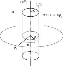
Fig. 1.: [LEFT] The pole configuration. [RIGHT] (6D) Riemann scalar curvature ${\hat{R}}/\alpha^{2}$ in the 6th order approximation. The horizontal axis is $k\rho$.

$M(>0)$ is the 6D Planck mass and is regarded as the fundamental scale of this dimensional reduction scenario. We take the line element: ${ds}^{2}={\rm e}^{-2\sigma(\rho)}\eta_{\mu\nu}dx^{\mu}dx^{\nu}+{d\rho}^{2}+\rho^{2}{\rm e}^{-2\omega(\rho)}d\varphi^{2}$ ($0\leq\rho<\infty{\quad,}\quad 0\leq\varphi<2\pi$), where $\eta_{\mu\nu}=\mbox{diag}(-1,1,1,1)$. In this choice, the 4D Poincaré invariance is preserved. Two ”warp” factors ${\rm e}^{-2\sigma(\rho)}$ and ${\rm e}^{-2\omega(\rho)}$ appear. The complex scalar field $\Phi$ is periodic with repect to $\varphi$. Taking a simple case : $\Phi_{m}(\rho,\varphi)=P(\rho){\rm e}^{im\varphi}$, ($m=0,\pm 1,\pm 2,\cdots$), the Einstein equation reduces to $3\sigma^{\prime\prime}-\frac{\sigma^{\prime}}{\rho}+\sigma^{\prime}\omega^{\prime}+\omega^{\prime\prime}-(\omega^{\prime})^{2}+2\frac{\omega^{\prime}}{\rho}=2M^{-4}{P^{\prime}}^{2}$; $-16{\sigma^{\prime}}^{2}+4\frac{\sigma^{\prime}}{\rho}-4\sigma^{\prime}\omega^{\prime}+4\sigma^{\prime\prime}=2M^{-4}V$; $4\sigma^{\prime\prime}-10{\sigma^{\prime}}^{2}=M^{-4}({P^{\prime}}^{2}-m^{2}\frac{{\rm e}^{2\omega}}{\rho^{2}}P^{2}+V)$.

The boundary condition, at $\rho=\infty$(infrared region), for $P(\rho)$ is taken as : $\rho\rightarrow\infty,\ P(\rho)\rightarrow+{v_{0}}.$ As for $\sigma$ and $\omega$, we assume (from the ”experience” in 5D Randall-Sundrum model[1, 2, 5, 6]) $\sigma^{\prime}\rightarrow a(\mbox{const}),\omega^{\prime}\rightarrow b(\mbox{const})$ as $\rho\rightarrow\infty$. Then, from the Einstein equations, we can deduce $m=0$ and $\sigma^{\prime}\rightarrow\alpha\ ,\omega^{\prime}\rightarrow\alpha\ ,\alpha=+\sqrt{\frac{-\Lambda}{10}}M^{-2}$ as $\rho\rightarrow\infty$. Note that the present asymptotic requirement demands the isotropic property around the $\rho=0$ axis ($m=0$), that is, the pole configuration. See Fig.1. In the above result we must have the condition: $\Lambda<0$ (Anti de Sitter). We can also fix the boundary condition at $\rho=+0$(ultra-violet region) based on the power-behavior assumption and ${\hat{R}}$ regularity: As $\rho\rightarrow+0$, the three functions $\sigma^{\prime},\omega^{\prime}$ and $P$ goes like  $\sigma^{\prime}\rightarrow s\rho^{a}\ ,\ \omega^{\prime}\rightarrow w\rho^{b}\ ,\ P\rightarrow x\rho^{c}$ where $s,w$ and $x$ are some constants ($s\neq 0,w\neq 0$), and $a=b=1\ ,\ c=0\ ,\ s=\frac{\lambda}{16}(x^{2}-{v_{0}}^{2})^{2}+\frac{\Lambda}{4}$.

Let us take the following form for $\sigma^{\prime}(\rho),\omega^{\prime}(\rho)$ and $P(\rho)$ as a solution.

$$\sigma^{\prime}(\rho)=\alpha\sum_{n=0}^{\infty}\frac{c_{2n+1}}{(2n+1)!}\{\tanh(k\rho)\}^{2n+1}\ ,\$$

$$\omega^{\prime}(\rho)=\alpha\sum_{n=0}^{\infty}\frac{d_{2n+1}}{(2n+1)!}\{\tanh(k\rho)\}^{2n+1}\ ,\ P(\rho)=v_{0}\sum_{n=0}^{\infty}\frac{e_{2n}}{(2n)!}\{\tanh(k\rho)\}^{2n}\ .$$ (2)

A new mass scale $k(>0)$ is introduced here and $1/k$ is the ”thickness” of the pole. The parameter $k$, with $M$ and $\rho_{c}$(defined later), plays a central role in this dimensional reduction scenario. The distortion of 6D space-time by the existence of the pole should be sufficiently small so that the quantum effect of 6D gravity can be ignored and the present classical analysis is valid. This requires the condition[1]: $k\ll M$.

The infrared boundary conditions require the coefficient-constants of (2) to have the following constraints

$$1=\sum_{n=0}^{\infty}\frac{c_{2n+1}}{(2n+1)!}{\quad,}\quad 1=\sum_{n=0}^{\infty}\frac{d_{2n+1}}{(2n+1)!}{\quad,}\quad 1=\sum_{n=0}^{\infty}\frac{e_{2n}}{(2n)!}{\quad.}$$ (3)

We solve these constraints. All coefficients are fixed except one free parameter $e_{0}$($=P(0)/v_{0}$). The first two orders are concretely given as

$$\begin{array}[]{cc}c_{1}=\frac{M^{-4}}{4k\alpha}\{\frac{\lambda{v_{0}}^{4}(1-{e_{0}}^{2})^{2}}{4}+\Lambda\},&c_{3}=\frac{3\lambda^{2}{v_{0}}^{6}}{32k^{3}\alpha}M^{-4}{e_{0}}^{2}(1-{e_{0}}^{2})^{2}+c_{1}(2+\frac{5\alpha}{k}c_{1}),\\ d_{1}=-\frac{2c_{1}}{3},e_{0}:\mbox{free parameter},&d_{3}=-\frac{4c_{1}}{3}(1+\frac{5\alpha c_{1}}{k}),e_{2}=-\frac{\lambda{v_{0}}^{2}}{4k^{2}}{e_{0}}(1-{e_{0}}^{2}).\end{array}$$ (6)

The general terms $(c_{2n+1},d_{2n+1},e_{2n}),n\geq 2$ are obtained in [3]. All coefficients are expressed by four parameters $\lambda,{v_{0}},\Lambda$ and $e_{0}$. The four ones have three constraints (3) from the boundary condition at the infrared infinity. Hence the present solution is one-parameter family solution. For an input value $e_{0}=-0.8$, the solution is concretely obtained as in Fig.1[RIGHT] and in Fig.2[LEFT]. Furthermore they are checked by the numerical method (Runge-Kutta) in Fig.2[RIGHT] where no assumption is made about the form of the solution. From the above solution (6), we can easily estimate the behavior of the vacuum parameters ($\Lambda,{v_{0}},\lambda$) near the 4D world limit (thin pole limit) as : $-\Lambda\sim M^{4}k^{2}$, ${v_{0}}\sim M^{2}$, $\lambda\sim M^{-4}k^{2}$, as $k\rightarrow\infty$. As for the $k$-dependence, this result is the same as the 5D model of Randall and Sundrum[1, 5].

3. Physical constants and See-Saw relation

Let us consider the case that the 4D geometry is slightly fluctuating around the Minkowski (flat) space: ${ds}^{2}={\rm e}^{-2\sigma(\rho)}g_{\mu\nu}dx^{\mu}dx^{\nu}+{d\rho}^{2}+\rho^{2}{\rm e}^{-2\omega(\rho)}d\varphi^{2},\ g_{\mu\nu}=\eta_{\mu\nu}+h_{\mu\nu}.$ The gravitational part of 6D action (1) reduces to 4D action as

$$\int d^{6}X\sqrt{-G}M^{4}{\hat{R}}\sim M^{4}\int_{0}^{2\pi}d\varphi\int_{0}^{\rho_{c}}d\rho\,\rho{\rm e}^{-2\sigma(\rho)-\omega(\rho)}\int d^{4}x\sqrt{-g}R+\cdots{\quad,}$$ (7)

where the infrared regularization parameter $\rho_{c}$ is introduced. $\rho_{c}$ specifies the size of the extra 2D space. Using the asymptotic forms, $\sigma\sim\alpha\rho,\ \omega\sim\alpha\rho$ as $\rho\rightarrow\infty$ and $\alpha=\sqrt{\frac{-\Lambda}{10}}M^{-2}\sim k$ as $k\rightarrow\infty$, we can evaluate $M_{pl}$ as : ${M_{pl}}^{2}\sim M^{4}2\pi\int_{0}^{\rho_{c}}d\rho\,\rho\,{\rm e}^{-3\alpha\rho}\sim\frac{M^{4}}{\alpha^{2}}\sim\frac{M^{4}}{k^{2}}$, where we have used the 4D reduction condition: $k\rho_{c}\gg 1$. (This result is different from 5D model[1, 5]: ${M_{pl}}^{2}\sim\frac{M^{3}}{k}$.) Writing the above result as $M_{pl}/{M}\sim M/k$, we notice this mass relation is the geometrical see-saw relation corresponding to the 2 by 2 matrix : ($0,\ M$ // $M,\ M_{pl}$). This provides the geometrical approach to the see-saw mechanism which is usually explained by the diagonalization of the (neutrino) mass matrix. ( See a textbook[7].) Similarly the 4D cosmological constant $\Lambda_{4d}$ is evaluated as $\Lambda_{4d}\sim\frac{\Lambda}{\alpha^{2}}\sim-M^{4}<0\ ,\ k\rho_{c}\gg 1\ .$ Using the value $M_{pl}\sim 10^{19}$GeV , the ”rescaled” cosmological parameter ${\tilde{\Lambda}}_{4d}\equiv\Lambda_{4d}/{M_{pl}}^{2}$ has the relation: $\sqrt{-{\tilde{\Lambda}}_{4d}}\sim k\sim M^{2}\times{10}^{-19}\ \mbox{GeV}\ .$ The unit of mass is GeV here and in the following. The observed value of $\sqrt{|{\tilde{\Lambda}}_{4d}|}$ is roughly ${10}^{-41}$.[8]

Some typical cases are 1) ($k={10}^{-41},M={10}^{-11}$), 2) ($k={10}^{-13},M={10}^{3}$) 3) ($k=10,M={10}^{10}$) 4) ($k={10}^{4},M={10}^{11.5}$) and 5) ($k={10}^{19},M={10}^{19}$). Cases 3) and 4) are moderate cases which are acceptable except for the cosmological constant. At present any choice of ($k,M$) looks to have some trouble if we take into account the cosmological constant. We consider the observed cosmological constant value should be explained by some unknown mechanism. As in the Callan and Harvey’s paper[9], we can have the 4D massless chiral fermion bound to the wall by introducing 6D Dirac fermion $\psi$ into (1). If we regulate the extra axis by the finite range $0\leq y\leq\rho_{c}$, the 4D fermion is expected to have a small mass $m_{f}\sim k{\rm e}^{-k\rho_{c}}$. If we take case 4) and regard the 4D fermion as a neutrino ($m_{\nu}\sim{10}^{-11}-{10}^{-9}\mbox{GeV}$), we obtain $\rho_{c}=(3.45-2.99)\times{10}^{-3}\mbox{GeV}^{-1}$. When the quarks or other leptons ($m_{q},m_{l}\sim 10^{-3}-10^{2}\mbox{GeV}$) are taken as the 4D fermion, we obtain $\rho_{c}=(1.61-0.461)\times{10}^{-3}$GeV^-1. It is quite a fascinating idea to identify the chiral fermion zero mode bound to the pole with the neutrinos, quarks or other leptons.

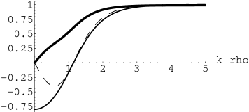
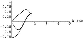
Fig. 2.: Horizontal axis: $k\rho$. [LEFT] The analytic results of $\omega^{\prime}/\alpha$(bold line), $\sigma^{\prime}/\alpha$(dashed line) and $P/{v_{0}}$(normal line). $e_{0}=-0.8$. The graphs are depicted in the 6-th order approximation. [RIGHT] The numerical results for $\omega^{\prime}/\alpha$(top), $\sigma^{\prime}/\alpha$(middle) and $P/{v_{0}}$(down). They are obtained by Runge-Kutta method. The initial point is $k\rho=0.1$. The initial values are borrowed from the analytical results.

4. Discussion and conclusion

We add some numerical fact about the see-saw relation. In the case 1), the value of $M$ ($\sim 10^{-11}$GeV) is the order of the neutrino mass. This choice looks ridiculous because the space-time behaves as six dimensional at the cosmological scale. The choice is, however, attractive in that it gives the right value of the cosmological constant. If this numerical fact is not accidental and has meaning, it says the cosmological size is related to the neutrino mass when it is ”see-sawed” with the Planck mass. These three fundamental scales could be geometrically related. We hope the results of the present hierarchy model will lead to develop further rich possibilities in the cosmology.

Bibliography

[1] L.Randall and R.Sundrum,
Phys.Rev.Lett. 83(1999)3370,hep-ph/9905221
[2] L.Randall and R.Sundrum,
Phys.Rev.Lett. 83(1999)4690,hep-th/9906064
[3] S.Ichinose,Univ.of Shizuoka preprint,
US-00-11, hep-th/0012255,”Pole Solution in Six Dimensions and Mass Hierarchy”
[4] S. Ichinose, Phys.Rev. D64(2001)025012
[Erratum ibid.D65(2001)029901], hep-th/0103211