New conformally flat initial data for spinning black holes

Abstract

We obtain an explicit solution of the momentum constraint for conformally flat, maximal slicing, initial data which gives an alternative to the purely longitudinal extrinsic curvature of Bowen and York. The new solution is related, in a precise form, with the extrinsic curvature of a Kerr slice. We study these new initial data representing spinning black holes by numerically solving the Hamiltonian constraint. They have the following features: i) Contain less radiation, for all allowed values of the rotation parameter, than the corresponding single spinning Bowen-York black hole. ii) The maximum rotation parameter $J/m^{2}$ reached by this solution is higher than that of the purely longitudinal solution allowing thus to describe holes closer to a maximally rotating Kerr one. We discuss the physical interpretation of these properties and their relation with the weak cosmic censorship conjecture. Finally, we generalize the data for multiple black holes using the “puncture” and isometric formulations.

I Introduction

Black holes are expected to be common objects in the universe. At the classical level, they are described by the Einstein field equations. The study of black holes by an initial value formulation of Einstein’s equations is a difficult problem, both from the analytic and numerical point of view. One of the most important open question regarding black holes is the weak cosmic censorship conjecture (cf. Penrose (1969) and also the recent review Wald (1999)): generic singularities of gravitational collapse are contained in black holes. The physical relevance of the concept of black holes depends on the validity of this conjecture. However, a general proof of the cosmic censorship conjecture lies outside the scope of present mathematical techniques. Thus, it is only possible to prove it in some very restrictive cases such spherical symmetry Christodoulou (1999) or to find indirect evidence of its validity. In the obtaining of these indirect evidences, a key role is played by the following three consequences of the weak cosmic censorship and the theory of black holes Hawking and Ellis (1973) Wald (1984):

• Every apparent horizon must be entirely contained within the black hole event horizon.

• If matter satisfies the null energy condition (i.e. if $T_{ab}k^{a}k^{b}\geq 0$ for all null $k^{a}$), then the area of the event horizon of a black hole cannot decrease in time.

• All black holes eventually settle down to a final Kerr black hole.

From (i)-(iii) we can deduce the Penrose inequality Penrose (1973)

$$A\leq 16\pi m^{2},$$ (1)

where $A$ is the area of the apparent horizon and $m$ is the total ADM mass of the space-time. Remarkably, the inequality (1) involves only quantities which can be computed directly form the initial data. After considerable effort, the Penrose inequality has been proved for time symmetric initial data Huisken and Ilmanen (2002)Bray (1999), providing an important support for the validity of (i)-(iii). The Penrose inequality can be strengthened if we assume axial symmetry and take into account angular momentum. Angular momentum is a conserved quantity in axially symmetric space-times, since it can be defined by a Komar integral (cf. Komar (1959) and also Wald (1984)). Using this fact and (i)-(iii) we deduce the following inequality Hawking (1972)

$$\epsilon_{A}\leq 1,\quad\epsilon_{A}\equiv\frac{A}{8\pi(m^{2}+\sqrt{m^{4}-J^{2}})},$$ (2)

where $J$ is the total angular momentum of the space-time. The inequality (2) must hold for every axially symmetric, non singular, asymptotically flat initial data. The equality in (2) must be achieved if and only if the data are slices of Kerr. Note that (2) implies

$$\epsilon_{J}\leq 1,\quad\epsilon_{J}\equiv\frac{J}{m^{2}},$$ (3)

We can also obtain upper bounds for the total amount of gravitational radiation emitted by the system. The total energy radiated is given by $E=m-m_{f}$ where $m_{f}$ is the mass of the final Kerr black hole. Since $m_{f}^{2}\geq J$ we have

$$\frac{E}{m}\leq 1-\sqrt{\epsilon_{J}}.$$ (4)

In contrast with (2) and (3), the inequality (4) involves the complete evolution of the initial data.

No analytic proof is available so far for (2). On the other hand if the inequality (2) fails for some initial data then, these data represent a counter example of weak cosmic censorship. Beside the trivial example of Kerr initial data, inequality (2) has been only studied in the spinning Bowen-York initial data (cf. York and Piran (1982), Choptuik and Unruh (1986), Cook and York (1990)). The spinning Bowen-York data Bowen and York (1980) are conformally flat and the second fundamental form is a explicit solution of the momentum constraint which contain the angular momentum of the data as a free parameter. The mass of the data has to be computed numerically by solving the Hamiltonian constraint. Remarkably, these data reach a limit in $\epsilon_{A}$ and $\epsilon_{J}$

$$0.812\lesssim\epsilon_{A}\leq 1,\quad\epsilon_{J}\lesssim 0.928.$$ (5)

$\epsilon_{A}$ reaches the upper limit only in the nonrotating case, since in this case the Bowen-York data reduce to the Schwarzschild data. $\epsilon_{J}$ cannot reach the limit case $1$ because they are not slices of Kerr for any choice of the free parameter $J$, even when $J$ goes to infinity. It appears that the Kerr metric admits no conformally flat slices (in fact, in Garat and Price (2000) it has been shown that there does not exist axisymmetric, conformally flat foliations of the Kerr spacetime that smoothly reduce, in the Schwarzschild limit, to slices of constant Schwarzschild time). It is rather easy to construct conformally flat data with smaller $\epsilon_{J}$: take the conformal second fundamental form of Bowen-York $K^{ab}_{BY}$ and add a solution of the momentum constraint $K^{ab}_{R}$ such that it has no angular momentum and such that the square of the sum $K^{ab}_{BY}+K^{ab}_{R}$ is bigger than the square of $K^{ab}_{BY}$ (these solutions can be explicitly constructed using Theorem 14 of Dain and Friedrich (2001)). Solve the Hamiltonian constraint with respect to the new second fundamental form $K^{ab}_{BY}+K^{ab}_{R}$. Then the new data will have bigger mass and equal angular momentum than the Bowen-York one.

It can be proved that it is not possible to reverse this argument to produce a data with bigger $\epsilon_{J}$. Because of this, one is tempted to believe that (5) is the upper limit to all conformally flat initial data. We will see that this is not the case.

In order to test inequalities (2)–(4) in a sharper way than with the Bowen-York data we need to construct data with higher $\epsilon_{A}$ and $\epsilon_{J}$. To do this, it is natural to consider perturbations of the Kerr initial data. However there are many ways to perturb the Kerr initial data, and for each case we have to deal with the solvability of a nonlinear elliptic equation in order to get a solution of the constraints. We have found a remarkable simple way of solving this problem. In this article we describe the construction of a conformally flat initial data in which the second fundamental form is related to the Kerr second fundamental form in a simple way. The second fundamental form will be an explicit solution of the momentum constraint with the following property: It is a conformal rescaling of the Kerr second fundamental form. These new data can be interpreted as a conformally flat deformation of the Kerr initial data. We find that for the new data

$$0.813\lesssim\epsilon_{A}\leq 1,\quad\epsilon_{J}\lesssim 0.932.$$ (6)

We also find that the total energy radiated is smaller than the Bowen-York one and satisfies the inequality (4).

The initial data presented here is also relevant for the binary problem. In order to improve the reliability of the results found in Baker et al. (2001) it is necessary to explore other family of initial data to know whether these results depend or not on the specific data used; that is, whether there exist physical properties of the wave form emitted by a binary system that are invariant under small changes on the data. It will be possible to measure only this kind of properties. Recently, other families of initial data has been suggested (see for instance Ref. Dain (2001a)Dain (2001b) and Bishop et al. (1998) Marronetti and Matzner (2000) for a Kerr-Schild type). The data constructed here is as simple as the standard Bowen-York, they will be a good candidate for future test and comparison with other initial data.

In Sec. II we construct a explicit solutions of the momentum constraint for conformally flat metrics such that they are conformal to the Kerr second fundamental form. These solution are constructed in an invariant way, they will depend on a scalar function $\omega$ that can be explicitly calculated for the Kerr initial data. In Sec. III we describe the numerical computations of sequences of initial data and study the $\epsilon_{J}$ and $\epsilon_{A}$ for increasing values of $J$. We then numerically evolve these initial data to compute the total gravitational energy radiated to infinity in order to compare it with the Bowen-York solution (and the vanishing Kerr data). Finally in Sec. IV we discuss the extension of our solution to the binary (an multi) black hole case.

II Constraint equations with axial symmetry and the new data

The standard conformal method for solving the constraints equations for maximal initial data is the following (cf. Choquet-Bruhat et al. (1999), Choquet-Bruhat and York (1980) and the reference given there). We give a conformal metric $h_{ab}$ and a symmetric trace free tensor $K^{ab}$ such that

$$D_{a}K^{ab}=0,$$ (7)

where $D_{a}$ is the covariant derivative with respect to $h_{ab}$. Then, we solve the following equation for the conformal factor $\varphi$

$$L_{h}\varphi=-\frac{{K}^{ab}{K}_{ab}}{8\varphi^{7}},$$ (8)

where $L_{h}=D^{a}D_{a}-R/8$, $R$ is the Ricci scalar of the metric $h_{ab}$ and the indexes are moved with $h_{ab}$. The physical fields defined by $\bar{h}_{ab}=\varphi^{4}h_{ab}$ and $\bar{K}^{ab}=\varphi^{-10}{K}^{ab}$ will satisfy the vacuum constraint equations. We need to prescribe appropriate boundary condition to equations (7) and (8), we will come back to this point later on.

Remarkable simplifications on (7) and (8) occur when $h_{ab}$ has a Killing vector $\eta^{a}$. We will assume that $\eta^{a}$ is hypersurface orthogonal and we define $\eta$ by $\eta=\eta^{a}\eta^{b}h_{ab}$. We analyze first the momentum constraint (7) (cf. Brandt and Seidel (1996), Baker and Puzio (1999) and Dain (2001b)) Consider the following vector field $S^{a}$

$$S^{a}=\frac{1}{\eta}\epsilon^{abc}\eta_{b}D_{c}\omega,\quad\pounds_{\eta}\omega=0,$$ (9)

where $\pounds_{\eta}$ is the Lie derivative with respect $\eta^{a}$ and $\epsilon_{abc}$ is the volume element of $h_{ab}$. It follows that $S^{a}$ satisfies

$$\pounds_{\eta}S^{a}=0,\quad S^{a}\eta_{a}=0,\quad D_{a}S^{a}=0.$$ (10)

Using the Killing equation $D_{(a}\eta_{b)}=0$, the fact that $\eta^{a}$ is hypersurface orthogonal, (i.e.; it satisfies $D_{a}\eta_{b}=-\eta_{[a}D_{b]}\ln\eta$) and equations (10) we conclude that the tensor

$${K}^{ab}=\frac{2}{\eta}S^{(a}\eta^{b)},$$ (11)

is trace free and satisfies (7). The square of ${K}^{ab}$ can be written in terms of $\omega$

$${K}^{ab}{K}_{ab}=2\frac{D_{c}\omega D^{c}\omega}{\eta^{2}}.$$ (12)

Two facts are important. First, the function $\omega$ is arbitrary. In particular it does not depend on the metric $h_{ab}$. Second, the extrinsic curvature of the Kerr initial data (in the Boyer-Lindquist coordinates) has the form (11), and then it has a corresponding function $\omega_{K}$.

We can describe now the new data. Let $h$ be the flat metric. Take the function $\omega_{K}$. Define ${K}^{ab}$ by (9) and (11). Solve (8) for the conformal factor with the appropriate boundary condition. We will obtain a conformally flat data with a extrinsic curvature that ‘resemble’ the Kerr extrinsic curvature. In other words, we use the function $\omega$ to construct out of the Kerr extrinsic curvature a explicit solution of the momentum constraint (7) for flat metric.

In order to write the equations and the boundary conditions explicitly we introduce spherical coordinates $(r,\theta,\phi)$, and write the metric in the form Brill (1959)

$$h=e^{-2q}(dr^{2}+r^{2}d\theta^{2})+r^{2}\sin^{2}\theta d\phi^{2}.$$ (13)

Then, the Hamiltonian constraint (8) reads

$$\Delta\varphi-\frac{\delta q}{4}\varphi=-\frac{(r\partial_{r}\omega)^{2}+(\partial_{\theta}\omega)^{2}}{4r^{6}\sin^{4}\theta\varphi^{7}},$$ (14)

where $\Delta$ is the flat Laplacian in the spherical coordinates $(r,\theta,\phi)$ and $\delta$ is the two-dimensional Laplacian

$$\delta q=\frac{1}{r}\partial_{r}(r\partial_{r}q)+\frac{1}{r^{2}}\partial^{2}_{\theta}q.$$ (15)

The Killing vector is given by $\eta^{a}=(\partial/\partial\phi)^{a}$, $\eta=r^{2}\sin^{2}\theta$ and $\pounds_{\eta}\omega=\partial_{\phi}\omega=0$. Note that $q$ and $\omega$ are almost free function. For $q$ we impose that is regular at the axis. Also, in order to have solutions for equation (14), we need to impose some global condition on $q$ (cf. Cantor and Brill (1981)). In our case, both condition are trivially satisfied since $q$ will be chosen to be zero. For the function $\omega$ we need that it cancel out the singular denominator $\sin^{4}\theta$ in (14), in order to obtain solutions which are smooth in $\theta$. The function $q$ determine the conformal metric, for $q=0$ we have that the data is conformally flat. The function $\omega$ determines the extrinsic curvature of the data.

To solve (14) we use the following boundary condition (cf. Friedrich (1988); Beig (1991); Brandt and Brügmann (1997) )

$$\lim_{r\rightarrow\infty}\varphi=1,\quad\lim_{r\rightarrow 0}r\varphi=\frac{m_{0}}{2},$$ (16)

where $m_{0}$ is a positive constant called bare mass. The total angular momentum of the data is given by

$$J=-\frac{1}{8\pi}\int_{S}S_{a}n^{a}\,dS,$$ (17)

where $S$ is any closed two-surface which enclose the origin. This equation can be written in a remarkable simple form in terms of $\omega$

$$J=\frac{1}{4}(\omega(r,\theta=\pi)-\omega(r,\theta=0)).$$ (18)

Let us mention some examples. The spinning Bowen-YorkBowen and York (1980) initial data is obtained as a solution of equation (14) with $q=0$, $m_{0}$ an arbitrary constant, and $\omega$ given by

$$\omega_{BY}=J(\cos^{3}\theta-3\cos\theta).$$ (19)

The Kerr initial data is obtained as a solution of (14), where the function $q$ is given by

$$e^{-2q_{K}}=\frac{\Sigma}{r_{BL}^{2}+a^{2}+\frac{2m_{K}a^{2}r_{BL}\sin^{2}\theta}{\Sigma}},$$ (20)

where

$$\Sigma=r^{2}_{BL}+a^{2}\cos^{2}\theta,$$ (21)

$$r_{BL}=r+m_{K}+\frac{m_{K}^{2}-a^{2}}{4r},$$ (22)

and $m_{K}$ and $a$ are the Kerr parameters, and $r_{BL}$ is the usual Brill-Lindquist radial coordinate. The function $\omega$ is given by

$$\omega_{K}=\omega_{BY}-\frac{m_{K}a^{3}\sin^{4}\theta\cos\theta}{\Sigma},$$ (23)

where, $J=m_{K}a$. And the parameter $m_{0}$ in Eq. (16) is given by

$$m_{0}=\sqrt{m_{K}^{2}-a^{2}}.$$ (24)

We see that the second fundamental form we are considering can be interpreted as a correction ${\cal O}(J^{3})$ (and higher) to that of Bowen and York as is directly reflected in the form of $\omega_{K}$.

The new data is $q=0$, and $\omega$ and $m_{0}$ given by Eqs. (23) and (24) respectively. The explicit components of the conformal second fundamental form are given by

$$K_{r\phi} =\frac{am_{K}\left[(r_{BL}^{2}-a^{2})\Sigma+2r_{BL}^{2}(r_{BL}^{2}+a^{2})\right]}{r^{2}\Sigma^{2}}\sin^{2}\theta,$$ (25)

$$K_{\theta\phi} =\frac{-2a^{3}m_{K}r_{BL}}{\Sigma^{2}}\left(1-\frac{m_{K}^{2}-a^{2}}{4r^{2}}\right)\cos\theta\sin^{3}\theta.$$

Note that $m_{0}$ is chosen such that we recover the Kerr initial data if we insert in equation (14) the corresponding function $q_{K}$.

Since $q=0$, in this case the boundary condition (16) can be achieved by the ansatz $\phi=1+m_{0}/(2r)+u$, where the function $u$ is bounded at the origin and satisfies the regular equation in $\mathbb{R}^{3}$

$$\Delta u=-\frac{r((r\partial_{r}\omega_{K})^{2}+(\partial_{\theta}\omega_{K})^{2})}{4\sin^{4}\theta(r+m_{0}/2+u)^{7}},$$ (26)

with the boundary condition $\lim_{r\rightarrow\infty}u=0$. This allows to use the ‘puncture’ treatment in numerical implementations of these initial data Brandt and Brügmann (1997). Existence and uniqueness of positive solution of the elliptic equation (26) can be proved by standard methods (see for example Choquet-Bruhat et al. (1999) and Dain and Friedrich (2001) and reference therein).

Finally, we want to prove that these data have an isometry defined by an inversion map through a sphere of radius $m_{0}/2$. Inversion transformation in the context of black holes initial data have been studied in Bowen and York (1980). The inversion map $I$ is defined in spherical coordinates by

$$r\rightarrow\left(\frac{m_{0}}{2}\right)^{2}\frac{1}{r},\quad\theta\rightarrow\theta,\quad\phi\rightarrow\phi.$$ (27)

We want to prove the following assertion: if the functions $\omega$ and $q$ satisfy

$$I\circ q=q,\quad I\circ\omega=\omega,$$ (28)

(that is, they are invariant under $I$); then the physical fields satisfy

$$(I^{*}\bar{h})_{ab}=\bar{h}_{ab},\quad(I^{*}\bar{K})_{ab}=-\bar{K}_{ab}.$$ (29)

In the examples presented here, one easily check that $\omega$ and $q$ satisfy Eq. (28), since their radial dependence is given in terms of $r_{BL}$ defined by Eq. (22), which satisfy $I\circ r_{BL}=r_{BL}$.

In order to prove the assertion, we first calculate the transformation of the conformal fields under $I$, from Eqs. (11) and (13) we obtain

$$(I^{*}h)_{ab}=\left(\frac{m_{0}}{2r}\right)^{4}h_{ab},\quad(I^{*}K)_{ab}=-\left(\frac{m_{0}}{2r}\right)^{-2}K_{ab}.$$ (30)

Then, using Eq. (8) we obtain

$$I\circ\varphi=\left(\frac{m_{0}}{2r}\right)^{-1}\varphi.$$ (31)

From Eqs. (30) and (31) follow Eqs. (29). This property of the data is used in the numerical calculations, as we will see in the following section.

III Numerical Results

The 2D fully nonlinear evolutions have been performed with a code, Magor, designed to evolve axisymmetric, rotating, highly distorted black holes, as described in Ref. Brandt and Seidel (1996, 1995). This nonlinear code solves the complete set of Einstein equations, in axisymmetry, with maximal slicing, for a rotating black hole. The code is written in a spherical-polar coordinate system, with a rescaled logarithmic radial coordinate that vanishes on the black hole throat. An isometry operator is used to provide boundary conditions on the throat of the black hole. The lapse is chosen to be antisymmetric across the throat. The shift vector components are employed to keep off diagonal components of the metric zero, except for the $g_{\theta\varphi}$. The initial data described in Sec. II above are provided through a fully nonlinear, numerical solution to the Hamiltonian constraint.

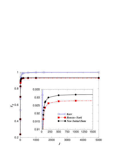
Figure 1: Rotation parameter $\epsilon_{J}$ as a function of the angular momentum $J$ for the new data, Kerr, and Bowen-York holes along the curve, keeping fixed the free parameter $m_{0}=2$. The curve for Kerr can be obtained analytically by equation (24).

In Fig. 1 we plot the curves of constant bare mass $m_{0}=2$ for initial data corresponding to rotating holes of Kerr, Bowen-York and the new ones introduced in this paper. Interestingly enough it was shown in Refs. Choptuik and Unruh (1986); Cook and York (1990) that the Bowen-York hole reach a maximum rotation parameter of $\epsilon_{J}\approx 0.928$ when $J$ goes to infinity. We have reproduced this curve as a function of $J$ reaching values of $J\approx 10,000$. For Kerr holes, along the curve $m_{0}=constant$ we have equation (24); the extreme Kerr $a/m_{K}=1$ correspond to the limit $J\rightarrow\infty$. We find for the data presented in this paper that the maximum lies near $\epsilon_{J}=0.932$, which is higher than the Bowen-York maximally rotating hole. This allows to study black hole evolutions from values closer to the maximally rotating Kerr ones.

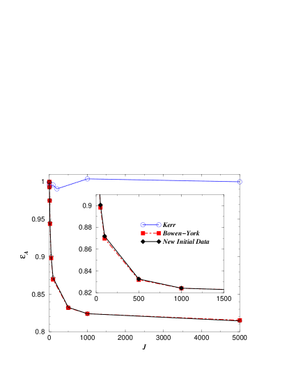
Figure 2: The horizon area parameter $\epsilon_{A}$ as a function of the angular momentum $J$ for the new data, Kerr, and Bowen-York holes along the curve, keeping fixed the free parameter $m_{0}=2$. For the Kerr initial data the exact value is $\epsilon_{A}=1$.

The code is able to evolve such data sets for time scales of roughly $t\leq 100m$, and study physics such as location and evolution of apparent horizons and gravitational wave emission. We have used typical grid sizes of 300 radial by 39 angular zones and extracted waves at the radial location $r_{obs}=15m$. The results are displayed in Fig. 3 and clearly show that the new data has less radiation content than the spinning Bowen-York holes. It produces roughly ten percent less the total radiated energy, $E$. Also this plot shows that inequality (4) is satisfied, the upper bound given by (4) is in this case $\approx 0.031$ while the maximum of the total energy radiated is $\approx 0.0015$.

For completeness we have plotted the evolution of Kerr initial data, for which the outgoing radiation should strictly vanish, as measure of the numerical error of our evolutions; and for comparison with future work we present the numerical parameters of our initial data family in Table 1.

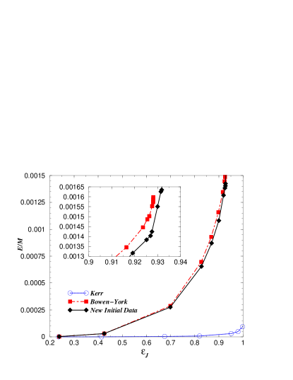
Figure 3: Radiation content of a single rotating black hole given by the new, Kerr and Bowen-York initial data. The upper bound given by (4) is in this case $\approx 0.031$.

Table 1: Initial spin $J$, ADM mass $m$, apparent horizon mass $m_{AH}=\sqrt{A/16\pi}$, and energy radiated of the new family of initial data

$J/(m_{0}/2)^{2}$	$m/(m_{0}/2)$	$m_{AH}/(m_{0}/2)$	$E/m$
1	2.0478	2.047	2.75e-6
2	2.1694	2.169	2.99e-5
5	2.674	2.668	0.00028
10	3.475	3.452	0.00066
20	4.743	4.686	0.00100
50	7.375	7.242	0.00131
100	10.386	10.165	0.00140
500	23.169	22.580	0.00162
1000	32.760	31.899	0.00163
5000	73.245	71.248	0.00191
10000	103.583	100.74	0.00187

IV Discussion

On the light of the two aspects studied in this paper we observe that the new data improves on the Bowen-York one leading to less spurious radiation and allowing a representation of higher rotating black holes while keeping the simplicity of the solutions, namely the explicit analytic form of the extrinsic curvature and conformal flatness of the three-geometry. This proves that even within the conformally flat ansatz one can look for astrophysically more realistic initial data. Also the new data satisfies inequalities (2), (3) and (4), supporting the validity of weak cosmic censorship.

We want to discuss now the generalization of these data for multiple black holes. In general, if the conformal metric $h_{ab}$ admits only one axial Killing vector $\eta^{a}$ the only freedom left is the choice of the origin in the $z=\cos\theta/r$ coordinate. By superposing different solutions of the momentum constraint of the form (11) such that they are singular at different points in the axis we will obtain a multiple black hole solution for a general axially symmetric metric. The spin of all of the black holes will point in the direction of the axis. However, when $h_{ab}$ is chosen to be the flat metric, then we have that a rotation about any axis is a Killing vector. Hence it is straightforward to generalize the data presented here to include multiple black holes in arbitrary location and with spin pointing in arbitrary direction. For completeness we will write explicitly the expression for the general solution of the momentum constraint, for flat metrics, with arbitrary origin and with spin pointing in arbitrary direction. The general Killing vector for the flat metric can be written as

$$\eta^{a}=\epsilon^{abc}\hat{z}_{b}(x_{c}-\bar{x}_{c}),\quad\eta=\rho^{2}-(\hat{z}_{c}(x^{c}-\bar{x}^{c}))^{2},$$ (32)

where $x_{c}$ are Cartesian coordinates, $\bar{x}^{c}$ and $\hat{z}^{a}$ are arbitrary constant vectors (we chose $\hat{z}^{a}$ to be a unit vector) and $\rho^{2}=(x^{c}-\bar{x}^{c})(x_{c}-\bar{x}_{c})$. The vector $\bar{x}^{c}$ represent the new origin and $\hat{z}^{a}$ the new axis. The new coordinate $\theta^{\prime}$ with respect to the axis $\hat{z}^{a}$ is given by

$$\cos\theta^{\prime}=\hat{z}_{c}(x^{c}-\bar{x}^{c}).$$ (33)

Fig. 4 displays explicitly those vectors.

Then, the desired expression for $K^{ab}$ is given again by Eqs. (11), (9) and (23) but we use in equations (11) and (9) the expression for $\eta^{a}$ and $\eta$ given by (32), and we replace in (23) $\theta$ by $\theta^{\prime}$ given by (33).

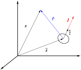
Figure 4: Geometry in the conformal (Cartesian) space of the location and orientation of a generic nth spinning black hole.