Illustrating Stability Properties of Numerical Relativity in Electrodynamics

Abstract

We show that a reformulation of the ADM equations in general relativity, which has dramatically improved the stability properties of numerical implementations, has a direct analogue in classical electrodynamics. We numerically integrate both the original and the revised versions of Maxwell’s equations, and show that their distinct numerical behavior reflects the properties found in linearized general relativity. Our results shed further light on the stability properties of general relativity, illustrate them in a very transparent context, and may provide a useful framework for further improvement of numerical schemes.

Motivated by the prospect of gravitational wave detections and the accompanying need for theoretical gravitational wave templates, much effort has recently gone into the development of numerical relativity algorithms that are capable of modeling the most promising sources of gravitational radiation, in particular the inspiral and coalescence of binary black holes and neutron stars. In the past, progress has been hampered by numerical instabilities that arise in straight-forward implementations of the traditional Arnowitt-Deser-Misner (ADM, adm62 ) $3+1$ decomposition of Einstein’s equations (e.g. bmss95 ; aetal98 ). These instabilities have been associated with the mathematical structure of the ADM equations, and as a cure a number of hyperbolic formulations have been suggested (e.g. bmss95 ; ay99 as well as r98 and references therein). Alternatively, Shibata and Nakamura sn95 and later Baumgarte and Shapiro bs99 suggested a reformulation of the ADM equations that has been demonstrated to dramatically improve the stability properties of numerical implementations (e.g. comparisons ). While the exact reason for this improvement is still somewhat mysterious (see aabss00 , hereafter AABSS, and math ), this new formulation, now often called the BSSN formulation, is quite widely used.

In this Brief Report we show that the BSSN reformulation of the ADM equations has a direct analogue in classical electrodynamics (E&M). We numerically implement both the original and the revised versions of Maxwell’s equations, and find that their distinct numerical properties reflect those found in general relativity (GR). As suggested by AABSS, these properties can be identified with the propagation of constraint violating modes. We present our findings in the hope that, in addition to being a very transparent illustration of the stability properties of GR, they may prove useful for the future development and improvement of numerical algorithms.

In a $3+1$ decomposition of GR, Einstein’s equations split into the two constraint equations

$$R-K_{ij}K^{ij}+K^{2}=2\rho$$ (1)

and

$$D_{j}K^{j}_{~{}i}-D_{i}K=S_{i}$$ (2)

and the two evolution equations

$$d_{t}\gamma_{ij}=-2\alpha K_{ij}$$ (3)

and

$$d_{t}K_{ij}=-D_{i}D_{j}\alpha+\alpha(R_{ij}-2K_{il}K^{l}_{~{}j}+KK_{ij}-M_{ij}).$$ (4)

Here $\gamma_{ij}$ is the spatial metric, $K_{ij}$ the extrinsic curvature, $K=\gamma^{ij}K_{ij}$ its trace, $\alpha$ and $\beta^{i}$ are the lapse function and the shift vector, and $\rho$, $S_{i}$ and $M_{ij}$ are matter source terms. The time derivative is defined as $d_{t}=\partial_{t}-{\mathcal{L}}_{\beta}$, and $R_{ij}$

$$R_{ij} = -\frac{1}{2}\gamma^{kl}\Big{(}\gamma_{ij,kl}+\gamma_{kl,ij}-\gamma_{kj,il}-\gamma_{il,kj}\Big{)}$$

$$+\gamma^{kl}\Big{(}\Gamma^{m}_{il}\Gamma_{mkj}-\Gamma^{m}_{ij}\Gamma_{mkl}\Big{)},$$

$D_{i}$ and $\Gamma^{i}_{jk}$ are the Ricci tensor, the covariant derivative, and the connection coefficients associated with $\gamma_{ij}$. Finally, $R$ is the scalar curvature $R=\gamma^{ij}R_{ij}$. Equations (1) through (4) are commonly refered to as the ADM equations adm62 .

The first term in the Ricci tensor (Illustrating Stability Properties of Numerical Relativity in Electrodynamics) is an elliptic operator acting on the components of the spatial metric $\gamma_{ij}$. If the Ricci tensor contained only this term, the two evolution equations (3) and (4) could be combined to form a wave equation for $\gamma_{ij}$. This property is spoiled by the appearance of the three other second derivative terms in (Illustrating Stability Properties of Numerical Relativity in Electrodynamics), suggesting that these terms may be responsible for the appearance of instabilities in many straight-forward, three-dimensional implementations of the ADM equations. This problem can be avoided by either using a hyperbolic formulation of GR (e.g. r98 ), or by eliminating the mixed second derivatives as in the BSSN formulation.

In this formulation, the conformally related metric $\bar{\gamma}_{ij}$ is defined as $\bar{\gamma}_{ij}=e^{-4\phi}\gamma_{ij},$ where the conformal factor $e^{\phi}$ is chosen so that the determinant of $\bar{\gamma}_{ij}$ is unity, $\bar{\gamma}=1$. The conformal exponent $\phi$ as well as the trace of the extrinsic curvature, $K$, are evolved as independent variables. Their evolution equations can be found from the traces of equations (3) and (4), while the trace-free parts of those equations form evolution equations for $\bar{\gamma}_{ij}$ and the trace-free part of the extrinsic curvature, $\bar{A}_{ij}$. The latter equation still contains the Ricci tensor $\bar{R}_{ij}$ associated with $\bar{\gamma}_{ij}$, which contains all the mixed second derivatives of (Illustrating Stability Properties of Numerical Relativity in Electrodynamics). The crucial step is to realize that these second derivatives can be absorbed in a first derivative of the “conformal connection functions”

$$\bar{\Gamma}^{i}\equiv\bar{\gamma}^{jk}\bar{\Gamma}^{i}_{jk}=-\bar{\gamma}^{ij}_{~{}~{},j},$$ (6)

where the last equality holds because $\bar{\gamma}=1$. Here and in the following all barred quantities are associated with $\bar{\gamma}_{ij}$. In terms of $\bar{\Gamma}^{i}$, the Ricci tensor can be written

$$\bar{R}_{ij} = -\frac{1}{2}\bar{\gamma}^{lm}\bar{\gamma}_{ij,lm}+\bar{\gamma}_{k(i}\partial_{j)}\bar{\Gamma}^{k}+\bar{\Gamma}^{k}\bar{\Gamma}_{(ij)k}+$$

$$\bar{\gamma}^{lm}\left(2\bar{\Gamma}^{k}_{l(i}\bar{\Gamma}_{j)km}+\bar{\Gamma}^{k}_{im}\bar{\Gamma}_{klj}\right)$$

(compare old_guys ). Evidently, the only remaining second derivative term is the elliptic operator $\bar{\gamma}^{lm}\bar{\gamma}_{ij,lm}$, if the $\bar{\Gamma}^{i}$ are considered as independent functions. For that purpose, an evolution equation is derived by permuting a time and space derivative in (6)

$$\partial_{t}\bar{\Gamma}^{i}=-\partial_{j}\Big{(}2\alpha\bar{A}^{ij}-2\bar{\gamma}^{m(j}\beta^{i)}_{~{},m}+\frac{2}{3}\bar{\gamma}^{ij}\beta^{l}_{~{},l}+\beta^{l}\bar{\gamma}^{ij}_{~{}~{},l}\Big{)}.$$ (8)

The divergence of the extrinsic curvature can now be eliminated with the help of the momentum constraint (2), which yields the evolution equation

$$\partial_{t}\bar{\Gamma}^{i}=-2\bar{A}^{ij}\partial_{j}\alpha$$ (9)

$$~{}~{}+2\alpha\Big{(}\bar{\Gamma}^{i}_{jk}\bar{A}^{kj}-\frac{2}{3}\bar{\gamma}^{ij}\partial_{j}K-\bar{\gamma}^{ij}S_{j}+6\bar{A}^{ij}\partial_{j}\phi\Big{)}$$

$$~{}~{}+\beta^{j}\bar{\partial}_{j}\Gamma^{i}-\bar{\Gamma}^{j}\partial_{j}\beta^{i}+\frac{2}{3}\bar{\Gamma}^{i}\partial_{j}\beta^{j}+\frac{1}{3}\bar{\gamma}^{li}\beta^{j}_{,jl}+\bar{\gamma}^{lj}\beta^{i}_{,lj}.$$

As in bs99 we will refer to the ADM equations (1) through (4) as System I, and to the new BSSN system of equations as System II. A complete listing and derivation of the latter can be found in bs99 .

Figure 1: The integrated constraint violation $\|\mathcal{C}\|\equiv(\int\mathcal{C}^{2}dV)^{1/2}$ for evolutions using Lorentz gauge with resolution $32^{3}$ and $64^{3}$ with outer boundaries at 4 (OB4) and 8 (OB8).

In an effort to better understand the improved numerical behavior of System II, AABSS linearized Systems I and II and identified their characteristic structure. They found that System I has constraint violating modes with a characteristic speed of zero. In System II, the characteristic speed of these modes changes to the speed of light. AABSS further demonstrated that in a non-linear model problem the existence of non-propagating, constraint violating modes may lead to numerical instabilities, as encountered in implementations of System I. Their analysis also demonstrated that the usage of the momentum constraint in the derivation of (9) is crucial for the characteristic speed for the constraint-violating mode to change to a non-zero value, and hence for the stability of the system. In the following we will show that very similar properties can be found in E&M.

In terms of a vector potential $A_{i}$, Maxwell’s equations can be written as the evolution equations

$$\partial_{t}A_{i} = -E_{i}-D_{i}\psi$$ (10)

$$\partial_{t}E_{i} = -D^{j}D_{j}A_{i}+D^{j}D_{i}A_{j}-4\pi j_{i},$$ (11)

and the constraint equation

$$D_{i}E^{i}=4\pi\rho_{e}.$$ (12)

Here $E^{i}$ is the electrical field, $\rho_{e}$ the charge density, $j_{i}$ the flux, and $\psi$ the scalar gauge potential. Identifying $A_{i}$ with $\gamma_{ij}$, $E_{i}$ with $K_{ij}$, and $\psi$ with $\beta^{i}$, we see that the structure of the evolution equations (10) and (11) is very similar to that of equations (3) and (4), and that the constraint equation (12) can be similarly identified with the momentum constraint (2). In analogy with GR, we refer to equations (10) through (12) as System I.

In further analogy, we will eliminate the mixed second derivative in (11) by introducing a new variable $\Gamma$

$$\Gamma\equiv D_{i}A^{i}$$ (13)

(compare (6)), in terms of which (11) becomes

$$\partial_{t}E_{i}=-D^{j}D_{j}A_{i}+D_{i}\Gamma-4\pi j_{i}.$$ (14)

As in (Illustrating Stability Properties of Numerical Relativity in Electrodynamics), the mixed second derivatives have been absorbed in a first derivative of the new variable. An evolution equation for $\Gamma$ can again be derived by permuting a time and space derivative in the definition of the new variable (13)

$$\partial_{t}\Gamma=D_{i}\partial_{t}A^{i}=-D_{i}E^{i}-D^{i}D_{i}\psi=-4\pi\rho_{e}-D^{i}D_{i}\psi.$$ (15)

Here we have used the constraint (12), which, as in GR, will turn out to be crucial (see (21) below). Equations (10), (14), (15) form the evolution equations of what we call System II. The definition (13) together with (12) form the constraint equations of System II.

For vanishing scalar potential $\psi=0$, an analytical vaccuum solution to Maxwell’s equations is given by the purely toriodal dipole field

$$A^{\hat{\phi}}={\mathcal{A}}\sin\theta\left(\frac{e^{-\lambda v^{2}}-e^{-\lambda u^{2}}}{r^{2}}-2\lambda\frac{ve^{-\lambda v^{2}}+ue^{-\lambda u^{2}}}{r}\right).$$ (16)

Here ${\mathcal{A}}$ is the amplitude, $\lambda$ parameterizes the size of the wavepackage, and $u$ and $v$ are the retarded and advanced time $u\equiv t+r$ and $v\equiv t-r$. According to (10), $E^{\hat{\phi}}$ can be found by taking a time derivative of (16). Since $\rho_{e}=0$ and $D_{i}A^{i}=0$ in this solution, $\psi=0$ is consistent with both the Coulomb gauge and the Lorentz gauge

$$\partial_{t}\psi=-D_{i}A^{i}-4\pi\rho_{e}=-\Gamma-4\pi\rho_{e}$$ (17)

(where the second equality applies for System II), if appropriate boundary and initial conditions are chosen. All results shown below were obtained with Lorentz gauge.

As initial data for our dynamical simulations we adopt the analytical solution (16) at $t=0$

$$A^{\hat{\phi}}=0,~{}~{}~{}E^{\hat{\phi}}=8{\mathcal{A}}r\sin\theta\lambda^{2}e^{-\lambda r^{2}}$$ (18)

with $\mathcal{A}=\lambda=1$ and transformed into cartesian coordinates.

We numerically implement System I and II following the algorithm of bs99 as closely as possible. In particular, we wrote the code in three spatial dimensions using cartesian coordinates. We use an iterative Crank-Nicholson scheme t00 to update the evolution equations, and impose outgoing wave boundary conditions on $E^{i}$, $A^{i}$ and $\Gamma$ as in bs99 . We verified that the numerical solution converges to the analytical solution to second order as long as the solution is not affected by the outer boundaries (which are first order accurate).

We compare the performance of System I and II by monitoring the constraint violation

$$\mathcal{C}\equiv D_{i}E^{i}-4\pi\rho_{e}.$$ (19)

In Fig. 1, we show integrated values $\|\mathcal{C}\|\equiv(\int\mathcal{C}^{2}dV)^{1/2}$ for Systems I and II for two different gridsizes ($32^{3}$ and $64^{3}$) and two different locations of the outer boundary (at 4 (OB4) and 8 (OB8)).

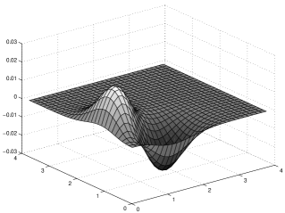
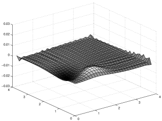
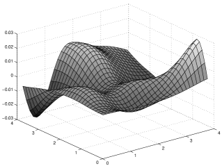
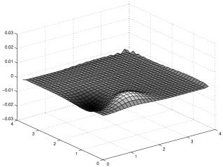
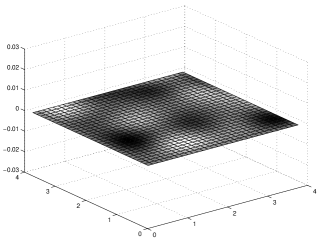
Figure 2: ${\mathcal{C}}$ in the z = .0625 plane (the first of our grid points) for System I (left column) and System II (right column) for a $32^{3}$ OB4 evolution in Lorentz gauge. We show results for $t=0$ (top row), $t=9.375$ (middle row) and $t=100$ (bottom row). ${\mathcal{C}}$ settles down to a constant profile in System I, but dissipates away in System II.

At early times, System I violates the constraint (12) to a lesser degree than System II. After about a light-crossing time, when the electro-magnetic wave has left the numerical grid, $\|\mathcal{C}\|$ settles down to a nearly constant value, which primarily depends on the grid-resolution. In System II, $\|\mathcal{C}\|$ is also largest after about a light-crossing time, but after that $\|\mathcal{C}\|$ decreases exponentially. As one might expect, the decay time of this exponential fall-off scales with the location of the outer boundary.

To further compare these Systems, we compare snapshots of the constraint violation ${\mathcal{C}}$ for the $32^{3}$ OB4 evolution in Fig. 2. With identical initial data, both Systems have identical values for ${\mathcal{C}}$ at $t=0$. At an intermediate time ${t=9.375}$, $\mathcal{C}$ is larger in System II than in System I, as one expects from Fig. 1. At a much later time (${t=200}$), however, System I has settled down to a constant shape, while $\mathcal{C}$ in System II has almost completely dissipated.

These numerical results demonstrate that, as in GR, the constraint violation ${\mathcal{C}}$ behaves very differently in the two systems. In E&M, this different behavior can be understood very easily from an analytic argument.

For System I, it is easy to show that a time derivative of the constraint violation (19) vanishes

$$\partial_{t}\mathcal{C}=D_{i}\partial_{t}E^{i}-4\pi\partial_{t}\rho_{e}=-4\pi(D_{i}j^{i}+\partial_{t}\rho_{e})=0,$$ (20)

where we have used the continuity equation $D_{i}j^{i}+\partial_{t}\rho_{e}=0$. This explains why at late times the profile of ${\mathcal{C}}$ remains unchanged in System I. This property is the analogue of AABSS’s finding that the linearized ADM equations have non-propagating, constraint violating modes.

For System II, on the other hand, it can be shown that ${\bf\mathcal{C}}$ satisfies a wave equation

$$\partial^{2}_{t}{\mathcal{C}} = \partial_{t}D^{i}\partial_{t}E_{i}-4\pi\partial^{2}_{t}\rho_{e}$$ (21)

$$= \partial_{t}D^{i}(-D_{j}D^{j}A_{i}+D_{i}\Gamma-4\pi j_{i})-4\pi\partial^{2}_{t}\rho_{e}$$

$$= -D^{i}(D_{j}D^{j}\partial_{t}A_{i}-D_{i}\partial_{t}\Gamma)-4\pi\partial_{t}(D^{i}j_{i}+\partial_{t}\rho_{e})$$

$$= D^{i}\Big{(}D_{j}D^{j}(E_{i}+D_{i}\psi)-D_{i}(4\pi\rho_{e}+D^{j}D_{j}\psi)\Big{)}$$

$$= D_{j}D^{j}(D^{i}E_{i}-4\pi\rho_{e})=D_{j}D^{j}{\mathcal{C}},$$

which explains why the constraint violations propagate away in System II. This is the analogue of AABSS’s finding that in the relativistic System II (the BSSN equations) the constraint violating modes propagate with the speed of light. Moreover, we now realize why the usage of the constraint (12) in (9) was crucial – without having made this substitution the terms on the last line of (21) would have cancelled, $\partial_{t}^{2}{\mathcal{C}}=0$, leading to a non-propagating constraint violation as in System I. The addition of constraint equations to the evolution equations has been found to be crucial in several other formulations of Einstein’s equations as well (e.g. ay99 ; constraint ).

To summarize, we see that the numerical stability properties of two formulations of GR are beautifully reflected in similar formulations of E&M. Maxwell’s equations therefore provide a very transparent framework for analyzing these properties, which may be useful for future algorithm development. For example, Fig. 2 shows that the outer boundaries produce much more noise in System I than in System II, which points to an inconsistency between the treatment of the interior equations and the boundary. Similar problems are likely to occur in GR, but might be easier to analyze in the simpler framework of E&M.

- (1) R. Arnowitt, S. Deser & C. W. Misner, in Gravitation: An Introduction to Current Research, edited by L. Witten (Wiley, New York, 1962).
- (2) C. Bona, J. Massó, E. Seidel & J. Stela, Phys. Rev. Lett. 75, 600 (1995).
- (3) A. M. Abrahams et. al., Phys. Rev. Lett. 80, 1812 (1998).
- (4) A. Anderson & J. W. York, Jr., Phys. Rev. Lett. 82, 4384 (1999).
- (5) O. Reula, Living Rev. Rel. 1, 3 (1998).
- (6) M. Shibata & T. Nakamura, Phys. Rev. D 52, 5428 (1995).
- (7) T. W. Baumgarte & S. L. Shapiro, Phys. Rev. D 59, 024007 (1999).
- (8) M. Alcubierre et. al., Phys. Rev. D 62, 044034 (2000); L. Lehner, M. Huq, & D. Garrison, Phys. Rev. D 62, 084016 (2000); M. Alcubierre & B. Brügmann, Phys. Rev. D 63, 104006 (2001).
- (9) M. Alcubierre, G. Allen, B. Brügmann, E. Seidel, & W.-M. Suen, Phys. Rev. D 62, 124011 (2000) (AABSS).
- (10) S. Frittelli & O. Reula, J. Math. Phys. 40, 5143 (1999); Miller, M., gr-qc/0008017 (2000).
- (11) T. De Donder, La gravifique einsteinienne (Gauthier-Villars, Paris, 1921); C. Lanczos, Phys. Z. 23, 537 (1922);
- (12) S. A. Teukolsky, Phys. Rev. D 61, 087501 (2000).
- (13) B. Kelly et. al., Phys. Rev. D 64, 084013 (2001); G. Yoneda & H. Shinkai, Phys. Rev. D 63 124019 (2001).