Post-Newtonian SPH calculations of binary neutron star coalescence. III. Irrotational systems and gravitational wave spectra

Abstract

Gravitational wave (GW) signals from coalescing binary neutron stars may soon become detectable by laser-interferometer detectors. Using our new post-Newtonian (PN) smoothed particle hydrodynamics (SPH) code, we have studied numerically the mergers of neutron star binaries with irrotational initial configurations. These are the most physically realistic initial conditions just prior to merger, since the neutron stars in these systems are expected to be spinning slowly at large separation, and the viscosity of neutron star matter is too small for tidal synchronization to be effective at small separation. However, the large shear that develops during the merger makes irrotational systems particularly difficult to study numerically in 3D. In addition, in PN gravity, accurate irrotational initial conditions are much more difficult to construct numerically than corotating initial conditions. Here we describe a new method for constructing numerically accurate initial conditions for irrotational binary systems with circular orbits in PN gravity. We then compute the 3D hydrodynamic evolution of these systems until the two stars have completely merged, and we determine the corresponding GW signals. We present results for systems with different binary mass ratios, and for neutron stars represented by polytropes with $\Gamma=2$ or $\Gamma=3$. Compared to mergers of corotating binaries, we find that irrotational binary mergers produce similar peak GW luminosities, but they shed almost no mass at all to large distances. The dependence of the GW signal on numerical resolution for calculations performed with $N\mathrel{\hbox{\hbox to0.0pt{\hbox{\lower 4.0pt\hbox{$\sim$}}\hss}\hbox{$>$}}}10^{5}$ SPH particles is extremely weak, and we find excellent agreement between runs utilizing $N=10^{5}$ and $N=10^{6}$ SPH particles (the largest SPH calculation ever performed to study such irrotational binary mergers). We also compute GW energy spectra based on all calculations reported here and in our previous works. We find that PN effects lead to clearly identifiable features in the GW energy spectrum of binary neutron star mergers, which may yield important information about the nuclear equation of state at extreme densities.

I Introduction and Motivation

Coalescing neutron star (NS) binaries are likely to be one of the most important sources of gravitational radiation for the ground-based laser-interferometer detectors in LIGO [1], VIRGO [2], GEO600 [3], and TAMA [4]. These interferometers are most sensitive to GW signals in the frequency range from about $10\,{\rm Hz}$ to $300\,{\rm Hz}$, which corresponds to the last several thousand orbits of the inspiral. During this period, the binary orbit is decaying very slowly, with the separation $r(t)$ and phase $\phi(t)$ following the standard theoretical treatment for the inspiral of two point masses (see, e.g., [5]). Theoretical templates for the corresponding quasi-periodic GW signals covering an appropriate range of values for the NS masses, as well as orbital phases and inclination angles, can be calculated to great precision (see, e.g., [6] and references therein), and template matching techniques can therefore be used to extract signals from noisy interferometer data. When the binary separation $r(t)$ has decreased all the way down to a few NS radii, the system becomes dynamically unstable [7] and the two stars merge hydrodynamically in $\sim 1\,$ms. The characteristic GW frequency of the final burst-like signal is $\mathrel{\hbox{\hbox to0.0pt{\hbox{\lower 4.0pt\hbox{$\sim$}}\hss}\hbox{$>$}}}1\,{\rm kHz}$, outside the range accessible by current broadband detectors. These GW signals may become detectable, however, by the use of signal recycling techniques, which provide increased sensitivity in a narrow frequency band [8]. These techniques are now being tested at GEO600, and will be used by the next generation of ground-based interferometers. Point-mass inspiral templates break down during the final few orbits. Instead, 3D numerical hydrodynamic calculations are required to describe the binary merger phase and predict theoretically the GW signals that will carry information about the NS equation of state (EOS).

The first hydrodynamic calculations of binary NS mergers in Newtonian gravity were performed by Nakamura, Oohara and collaborators using a grid-based, Eulerian finite-difference code [9]. Rasio and Shapiro ([10], hereafter RS) later used Lagrangian SPH calculations to study both the stability properties of close NS binaries and the evolution of dynamically unstable systems to complete coalescence. Since then, several groups have performed increasingly sophisticated calculations in Newtonian gravity, exploring the full parameter space of the problem with either SPH [11, 12, 13] or the Eulerian, grid-based piecewise parabolic method (PPM) [14, 15, 16], and focusing on topics as diverse as the GW energy spectrum [11], the production of r-process elements [13], and the neutrino emission as a possible trigger for gamma-ray bursts [16]. Some of these Newtonian calculations have included terms to model approximately the effects of the gravitational radiation reaction [16].

The first calculations to include the lowest-order (1PN) corrections to Newtonian gravity, as well as the lowest-order dissipative effects of the gravitational radiation reaction (2.5PN) were performed by Shibata, Oohara, and Nakamura, using an Eulerian grid-based method [17]. More recently, the authors ([18, 19], hereafter Paper 1 and Paper 2, respectively), as well as Ayal et al.[20], have performed PN SPH calculations, using the PN hydrodynamics formalism developed by Blanchet, Damour, and Schäfer ([21], hereafter BDS). These calculations have revealed that the addition of 1PN terms can have a significant effect on the results of hydrodynamic merger calculations, and on the theoretical predictions for GW signals. For example, Paper 1 showed a comparison between two calculations for initially corotating, equal-mass binary NS systems. In the first calculation, radiation reaction effects were included, but no 1PN terms were used, whereas a complete set of both 1PN and 2.5PN terms were included in the second calculation. It was found that the inclusion of 1PN terms affected the evolution of the system both prior to merger and during the merger itself. The final inspiral rate of the PN binary just prior to merger was much more rapid, indicating that the orbit became dynamically unstable at a greater separation. Additionally, the GW luminosity produced by the PN system showed a series of several peaks, absent from the Newtonian calculation.

Most previous hydrodynamic calculations of binary NS mergers have assumed corotating initial conditions, and many modeled the stars as initially spherical. However, real binary NS are unlikely to be described well by such initial conditions. Just prior to contact, tidal deformations can be quite large and the stars can have very nonspherical shapes [7]. Nevertheless, because of the very low viscosity of the NS fluid, the tidal synchronization timescale for coalescing NS binaries is expected to always be longer than the orbital decay timescale [22]. Therefore, a corotating state is unphysical. In addition, at large separation, the NS in these systems are expected to be spinning slowly (see, e.g., [23]; observed spin periods for radio pulsars in double NS systems are $\mathrel{\hbox{\hbox to0.0pt{\hbox{\lower 4.0pt\hbox{$\sim$}}\hss}\hbox{$>$}}}50\,$ms, much longer than their final orbital periods). Thus, the fluid in close NS binaries should remain nearly irrotational (in the inertial frame) and the stars in these systems can be described approximately by irrotational Riemann ellipsoids [7, 22, 24, 25]. In Paper 2, we showed that nonsynchronized initial conditions can lead to significant differences in the hydrodynamic evolution of coalescing binaries, especially in the amount of mass ejected as a result of the rotational instability that develops during the merger.

There are many difficulties associated with numerical calculations of binary mergers with irrotational initial conditions, especially in PN gravity. Foremost of these is the difficulty in preparing the initial, quasi-equilibrium state of the binary system. In synchronized binaries, the two stars are at rest in a reference frame which corotates with the system, and thus relaxation techniques can be used to construct accurately the hydrostatic equilibrium initial state in this corotating frame (see [10] and Paper 1). For irrotational systems, no such frame exists in which the entire fluid would appear to be in hydrostatic equilibrium. Instead, one must determine self-consistently the initial velocity field of the fluid in the inertial frame. Otherwise (e.g., when simple spherical models are used), spurious oscillations caused by initial deviations from equilibrium can lead to numerical errors. This is especially of concern in PN gravity, where the strength of the gravitational force at any point in the NS contains terms proportional to the gravitational potential and pressure at 1PN order.

Another serious problem for hydrodynamic calculations with irrotational initial conditions is the issue of spatial resolution and numerical convergence. As was first pointed out in RS2, in a frame corotating with the binary orbital motion, irrotational stars appear counterspinning so that, when they first make contact during the coalescence, a vortex sheet is formed along the interface. This tangential discontinuity is Kelvin-Helmholtz unstable at all wavelengths[26]. The sheet is expected to break into a turbulent boundary layer which propagates into the fluid and generates vorticity through dissipation on small scales. How well this can be handled by 3D numerical calculations with limited spatial resolution is unclear.

The outline of our paper is as follows. Section II presents a summary of our numerical methods, including a brief description of our PN SPH code, and an explanation of the method used to construct irrotational initial conditions in PN gravity. Additionally, we give the parameters and assumptions for all new calculations discussed in this paper. Section III presents our numerical results based on SPH calculations for several representative binary systems, all with irrotational initial configurations, but varying mass ratios and NS EOS. To test our numerical methods, we also study the effects of changing the initial binary separation and the numerical resolution. Section IV presents GW energy spectra calculated from the runs in this and previous papers, as well as a discussion of how the measurement of spectral features could constrain the NS EOS. A summary of our PN results and possible directions for further research, including the possibility of fully relativistic SPH calculations, are presented in Section V.

II Numerical Methods

A Conventions and Basic Parameters

All our calculations were performed using the post-Newtonian (PN) SPH code described in detail in Papers 1 and 2. It is a Lagrangian, particle-based code, with a treatment of relativistic hydrodynamics and self-gravity adapted from the PN formalism of BDS. As in our previous work, we use a hybrid 1PN/2.5PN formalism, in which radiation reaction effects are treated at full strength (i.e., corresponding to realistic NS parameters), but 1PN corrections are scaled down by a factor of about 3 to make them numerically tractable (see below). We did not perform any new Newtonian calculations for this paper. All the Poisson-type field equations of the BDS formalism are solved on grids of size $256^{3}$, including the space for zero-padding, which yields the proper boundary conditions. Shock heating, which is normally treated via an SPH artificial viscosity, was ignored, since it plays a negligible role in binary coalescence, especially for fluids with a very stiff EOS. All runs, except those used to study the effects of numerical resolution on our results, use $5\times 10^{4}$ SPH particles per NS (i.e., the total number of particles $N=10^{5}$), independent of the binary mass ratio $q$. The number of SPH particle neighbors is set to $N_{N}=100$ for all runs with $N=10^{5}$.

Unless indicated otherwise, we use units such that $G=M=R=1$, where $M$ and $R$ are the mass and radius of one NS. In calculations for unequal-mass binaries, we use the mass and radius of the primary. As in our previous papers, we compute the gravitational radiation reaction assuming that the speed of light $c_{2.5PN}=2.5$ in our units, which corresponds to a neutron star compactness $GM/Rc^{2}_{2.5PN}=0.16$. For a standard NS mass of $1.4\,M_{\odot}$ this also corresponds to a radius $R=13\,$km. The unit of frequency (used throughout Sec. IV) is then

$$f_{\rm dyn}\equiv\left(\frac{GM}{R^{3}}\right)^{1/2}=9.2\,{\rm kHz}\,\left(\frac{M}{1.4\,M_{\odot}}\right)^{1/2}\,\left(\frac{R}{13\,{\rm km}}\right)^{-3/2}$$ (1)

In order to keep all 1PN terms sufficiently small with respect to Newtonian quantities, we calculate them assuming a somewhat larger value of the speed of light, $c_{1PN}=4.47$, which would correspond to NS with $GM/Rc^{2}_{1PN}=0.05$.

As in our previous work, all calculations in this paper use a simple polytropic EOS, i.e., the pressure is given in terms of the mass-energy density by $P=k\rho_{*}^{\Gamma}$. We use $\Gamma=3$ to represent a typical stiff NS EOS, and $\Gamma=2$ to represent a somewhat softer EOS. The values of the polytropic constant $k$ for all our NS models (determined by the mass-radius relation) are the same as those used in Paper 2 (see Table 1 therein). Models for single NS are taken from Papers 1 and 2. It should be noted that models of NS with identical masses and polytropic constants but different numbers of SPH particles may have slightly different effective radii, due to numerical resolution effects near the stellar surface.

It is not easy to define a meaningful and accurate origin of time for merger calculations. The moment of first contact between the two stars is difficult to determine accurately, since it involves the smoothing lengths of particles located near the surface of each NS, where the method is least accurate. Therefore, following the convention in our earlier papers, we set the absolute timescale for each run by defining the moment of peak GW luminosity to be at $t=20$ in our units. Many runs therefore start at $t_{0}<0$, but this is merely a matter of convention.

B Constructing Irrotational Initial Configurations

To construct irrotational binary configurations in quasi-equilibrium, we start from our relaxed, equilibrium models for single NS (Paper 2, Sec. IIA). These models are transformed linearly into irrotational triaxial ellipsoids, with principal axes taken from the PN models of Lombardi, Rasio, and Shapiro for equilibrium NS binaries [24]. For example, for an equal-mass system containing two $\Gamma=3$ polytropes with an initial separation $r_{0}=4.0$, we find from their Table III that the principal axes are given by $a_{1}/R\simeq 1.02$, $a_{2}/a_{1}\simeq 0.96$, and $a_{3}/a_{1}\simeq 0.96$, where $a_{1}$, $a_{2}$, and $a_{3}$ are measured along the binary axis (x-direction), the orbital motion (y-direction), and the rotation axis (z-direction), respectively. For an initial separation $r_{0}=3.5$, we find $a_{1}/R\simeq 1.05$, $a_{2}/a_{1}\simeq 0.93$, and $a_{3}/a_{1}\simeq 0.93$. For the initial velocity field of the fluid we adopt the simple form assumed for the internal fluid motion in irrotational Riemann ellipsoids[7],

$$v_{x}=-\Omega y\left(1-\frac{2a_{1}^{2}}{a_{1}^{2}+a_{2}^{2}}\right)$$ (2)

$$v_{y}=\Omega x\left(1-\frac{2a_{2}^{2}}{a_{1}^{2}+a_{2}^{2}}\right),$$ (3)

where $\Omega$ is the orbital angular velocity. It is easy to verify that this initial velocity field has zero vorticity in the inertial frame.

Calculating self-consistently the correct value of $\Omega$ corresponding to a quasi-equilibrium circular orbit proves to be much more difficult in PN gravity than in Newtonian gravity, especially for irrotational configurations. In Newtonian gravity, the gravitational force between the two stars is independent of the magnitude of the tidal deformation of the bodies to lowest order. Thus, even if the initial configuration of matter in the binary is slightly out of equilibrium, the orbit calculated for the two stars will still be almost perfectly circular. In PN gravity, the situation is quite different. From Appendix A of Paper 1, we see that the gravitational acceleration,in our PN formalism, denoted there as $F_{grav}$, is calculated as

$$F_{grav}=(1+\frac{1}{c^{2}}\left[\frac{3\Gamma-2}{\Gamma-1}\frac{P}{r_{*}}-U_{*}+\frac{3w^{2}}{2}\right])\nabla U_{*}+\ldots,$$ (4)

where $w$ is the the 1PN-adjusted velocity, and $P$, $r_{*}$, and $U_{*}$ are the pressure, rest-mass density, and gravitational potential, respectively, as defined in the BDS formalism (note that $U_{*}$ as defined here is a positive quantity). The quantity in brackets is the 1PN correction to the gravitational force, and depends explicitly on the initial thermodynamic state of the NS. Small oscillations of each star about equilibrium result in errors when calculating the gravitational force felt by each component of the binary. In addition, the gravitational force is affected by the orbital velocity of the NS. Thus, when we try to calculate the orbital velocity from the centripetal accelerations of the respective NS, as in Eq. (1) of Paper 2,

$$\Omega=\sqrt{\frac{-\dot{v}^{(1)}_{x}+\dot{v}^{(2)}_{x}}{2r_{0}}},$$ (5)

where $v^{(1)}$ and $v^{(2)}$ are the center-of-mass velocities of the primary (located initially on the positive x-axis) and the secondary (located on the negative x-axis), respectively, we face the problem that the RHS of the equation is itself a function of $\Omega$.

For an initially synchronized system, we solve this problem by relaxing the matter in a frame corotating with the binary, and in the process find the equilibrium value of $\Omega$ self-consistently (See Paper 1, Appendix A). For an irrotational binary, this is not possible, since we cannot describe a priori the proper velocity field toward which the matter must relax. We solve the problem instead by a more direct method. Realizing that any simple approximation of the orbital velocity should be near the correct PN value, we alter the expression for $\Omega$ to include a correction factor which, we hope, will remove the effect of any small deviations away from equilibrium on the gravitational accelerations felt by each NS. Therefore, we introduce a parameter $\kappa$ such that

$$\Omega=\kappa\sqrt{\frac{-\dot{v}^{(1)}_{x}+\dot{v}^{(2)}_{x}}{2r_{0}}}.$$ (6)

For each value of $\kappa$, we iterate Eqs. 2, 3, and 6 over $\Omega$ to determine a self-consistent velocity field at $t=0$. We then perform trials for each value of $\kappa$, i.e., we perform purely dynamical integrations (with radiation reaction turned off) for about one full orbit, until we find one which produces a nearly circular orbit (such that $r(t)$ changes by no more than $1\%$). The results of one such set of calculations, for equal-mass NS with a $\Gamma=3$ EOS and an initial separation $r_{0}=4.0$, is shown in the top panel of Fig. 1. We see that for $\kappa=1.0$, which works extremely well for all runs performed in Newtonian gravity, the orbital angular velocity is too small, and the pericenter of the orbit lies within the dynamical stability limit, causing the system to merge (artificially) within the first orbital period. For $\kappa=1.2$, we see that the orbit is elliptical, with our initial state corresponding to pericenter. For a value of $\kappa=1.11$ we obtain a very nearly circular orbit. A residual small-amplitude oscillation is shown in greater detail in the middle panel of Fig. 1. We see that it occurs not on the orbital period timescale, but rather on the internal dynamical timescale of the stars. It is the direct result of small-amplitude pulsations of each NS about equilibrium. This is illustrated more clearly in the bottom panel of the figure, which shows the clear correlation between the radial acceleration of each NS (shown as a fraction of the total inward gravitational acceleration) and the central density of each NS. The numerical noise is an artifact of the small number of particles located near the very center of each star for the density curve, and of precision limits in the calculation for the acceleration curve. When averaged over time, we see nearly perfect correlation between the two quantities. Also shown in the middle panel of Fig. 1 is a thick solid line depicting the dynamical evolution of a run with $\kappa=1.11$ and radiation reaction included, to give a sense of the proper inspiral velocity in relation to the spurious radial velocities resulting from oscillations.

C Summary of calculations

We have performed several large-scale SPH calculations of NS binary coalescence, assuming an irrotational initial condition for the binary system. Table I summarizes the relevant parameters of all runs performed, listing the adiabatic exponent $\Gamma$, the mass ratio $q$, the initial separation $r_{0}$, and the number of SPH particles.

We continue to use the same nomenclature for our SPH runs introduced in Paper 2, although we present here a new run E1, using an improved initial configuration calculated by the method described in the previous section. Run E1 is for a system with a $\Gamma=3$ EOS, equal-mass NS, and an initial separation $r_{0}=4.0$, and is similar in all respects to run B1 of Paper 2 (called the PN run in Paper 1), except that the initial condition is irrotational. It was continued until a quasi-stationary remnant configuration was reached. Run E2 is for a system with the same $\Gamma=3$ EOS, but a mass ratio of $q=0.8$, and was started from a smaller initial separation $r_{0}=3.5$, since binaries with smaller masses take longer to coalesce. In runs F1 and F2, the EOS has $\Gamma=2$, but we use the same mass ratios and initial separations as runs E1 and E2, respectively.

Additionally, to assess the numerical accuracy and convergence of calculations for irrotational binaries, we performed three runs which were primarily designed to test the dependence of the physical results on numerical parameters. First, we performed one run, labeled T2, identical to E1 except for a smaller initial separation $r_{0}=3.5$. This run was used to study how accurately the irrotational flow is maintained during the early stages of inspiral, and the effects of a small amount of spurious tidal synchronization on the GW signal. We then repeated run T2 using $5000$ and $500,000$ SPH particles per NS (for a total of $N=10^{4}$ and $N=10^{6}$ particles, respectively), to study the effect of numerical resolution on calculations where we know small-scale instabilities will develop. The number of neighbors was adjusted in the two runs to be $N_{N}=50$ and $N_{N}=200$, respectively. This choice is dictated by the convergence and consistency properties of our basic SPH scheme: convergence toward a physically accurate solution is expected when both $N\rightarrow\infty$ and $N_{N}\rightarrow\infty$, but with $N_{N}/N\rightarrow 0$ [27]. The primary consideration behind the choice of the initial separation at $r_{0}=3.5$ (rather than $r_{0}=4.0$) was the high computational cost of a run with $N=10^{6}$.

III Numerical Results and Tests

A Overview

The coalescence process for binary NS systems is essentially the same qualitatively whether they are initially synchronized or irrotational. Prior to merger, both NS show tidal elongation as well as the development of a tidal lag angle $\theta_{lag}$, as noted in Papers 1 and 2, created as the NS continuously try to maintain equilibrium while the coalescence timescale gets shorter and shorter. The inner edge of each NS rotates forward relative to the binary axis, and the outer edge of each NS rotates backward. We define $\theta_{lag}$ to be the angle in the horizontal plane between the axis of the primary moment of inertia of each NS and the axis connecting the centers of mass of the respective NS. For equal-mass systems, the angle is the same for both NS. For binaries with $q<1$ we always find a larger lag angle for the secondary than the primary.

Mass shedding through the outer Lagrange points is suppressed in irrotational binaries, but the formation of a differentially rotating remnant is quite similar. That said, it is important to understand the different computational challenges presented by irrotational systems. To demonstrate this, in Fig. 2 we show the evolution of run E1, with a $\Gamma=3$ EOS, a mass ratio $q=1.0$, and an initial separation $r_{0}=4.0$. It is in all ways similar to run B1, except that the NS start from an irrotational configuration. Rather than plot SPH particle positions, we instead show the density contours of the matter in the orbital plane, overlaying the velocity of the material in the corotating frame, defined by taking a particle-averaged tangential velocity, such that

$$\Omega_{c}=\frac{\sum_{i}m_{i}[(xv_{y}-yv_{x})/r_{cyl}]_{i}}{\sum_{i}m_{i}(r_{cyl})_{i}},$$ (7)

where the cylindrical radius is defined as $r_{cyl}=\sqrt{x^{2}+y^{2}}$. In synchronized binaries, the material maintains only a small velocity in the corotating frame prior to first contact. In contrast, for irrotational binaries material on the inner edge of each NS is counterspinning in the corotating frame, and thus we see a large discontinuity in the tangential velocity when first contact is made. This surface layer, initially at low density, is Kelvin-Helmholtz unstable to the formation of turbulent vortices on all length scales. Meanwhile, material on the outer edge of each NS has less angular momentum in an irrotational binary configuration than in a synchronized one. Thus, there is less total angular momentum in the system, and mass shedding is greatly suppressed, as we will discuss further in Sec. III B. At late times, though, the remnant rotates differentially, with the same profile seen in the synchronized case, namely $\Omega(r)$ attaining its maximum value at the center of the remnant, and decreasing as a function of radius.

In Table II, we show some basic quantities pertaining our GW results, as well as the initial time for all runs, and the tidal lag angle $\theta_{lag}$ which existed at the moment of first contact. The negative values of $t_{0}$ merely reflect the fact that our runs require more than 20 dynamical times before reaching peak GW luminosity. Lag angles $\theta_{lag}$ are listed for the primary and secondary, respectively, in systems with $q\neq 1$. Each GW signal we compute typically shows an increasing GW luminosity as the stars approach contact, followed by a peak and then a decline as the NS merge together. Most runs then show a second GW luminosity peak of smaller amplitude. For all of our runs we list the maximum GW luminosity $L_{max}\equiv{\rm max}(L_{GW}(t)$ and maximum GW amplitude $h_{max}\equiv{\rm max}(\sqrt{h_{+}(t)^{2}+h_{\times}(t)^{2}})$, where $h_{+}$, $h_{\times}$, and $L_{GW}$ are defined by Eqs. (23)-(25) of Paper 1 (see also Eqs. 8 and 9 below). Quantities referring to the first and second luminosity peaks are denoted “1” and “2”, respectively. In addition, we show the time $t^{(2)}$ at which the second peak occurs.

We continued several of our runs to late times to study the full GW signal produced during the coalescence, as well as to study the properties of the merger remnants that may form in these situations. For each of these runs, we list several of the basic parameters of the merger remnant in Table III, using the values computed for the remnant at $t=65$. We identify the remnant mass $M_{r}$, defining the edge of the remnant by a density cut $r_{*}>0.005$, as well as the gravitational mass of the remnant in the PN runs, where the gravitational mass, which differs from the rest mass, is given by $M_{gr}\equiv\int r_{*}(1+\delta)d^{3}x$ (see Paper 1 for more details). Additionally, we list the Kerr parameter $a_{r}\equiv cJ_{r}/M_{gr}^{2}$, central and equatorial values of the angular velocity, $\Omega_{c}$ and $\Omega_{eq}$, the semi-major axis $a_{1}$ and ratios of the equatorial and vertical radii $a_{2}/a_{1}$ and $a_{3}/a_{1}$, and the ratio of the principal moments of inertia $I_{2}/I_{1}$.

B Dependence on EOS Stiffness

To study the effect of the EOS on the evolution of irrotational NS binaries, we calculated mergers of both $\Gamma=3$ and $\Gamma=2$ polytropes (runs E1 and F1, respectively). A comparison of the binary separations as a function of time, along with the dimensionless GW luminosities and amplitudes are shown in Fig. 3. Immediately apparent is a difference in the location of the dynamical stability limit found in the two calculations. The orbit of the binary system containing NS with a softer EOS (run F1) remains stable at separations where the binary system with the stiffer EOS has already begun to plunge inward dynamically. We see that, as in the synchronized case presented in Paper 2, the peak GW luminosity in dimensionless form is larger for the softer EOS, but after a secondary luminosity peak the remnant relaxes toward a spheroidal, non-radiating configuration (with essentially no emission whatsoever after $t\simeq 40$). We also note that the secondary peak occurs sooner after the primary peak, by a factor of $\simeq 30\%$.

Even though they are presumed to be unphysical, calculations started from a synchronized initial condition make up much of the body of work performed to date on the binary NS coalescence problem. Noting this, we compare our irrotational run E1, with parameters detailed above, to one similar in every respect but started with a synchronized initial condition, our run B1. In the top panel of Fig. 4, we see that the inspiral tracks do not align particularly well. Synchronized binaries contain more total energy, and are thus less dynamically stable than irrotational ones, leading to a more rapid inspiral, even before the stability limit is reached. Additionally, the binary separation “hangs up” earlier, at a separation $r\approx 2.0$, indicating the onset of mass shedding, as matter begins to expand radially outward from the system. The middle and bottom panels of the figure show the GW signals and luminosity, respectively, for the two runs. While the initial luminosity peaks are similar for both runs, both in amplitude and morphology, the secondary peaks are vastly different. The secondary peak for the synchronized system is of considerably greater magnitude than in the irrotational case, and delayed relative to it. We conclude that, while the adiabatic index seems to be the dominant factor in determining the GW signal during the merger itself, the initial velocity profiles of the NS play a key role in the evolution of the remnant, as well as affecting the orbital dynamics during inspiral.

To better understand the features found in the GW signals of these calculations, particle plots for runs E1, B1, and F1 are shown in Fig. 5. Comparing the leftmost panels, we see that at $t=20$, when the GW luminosity peaks, the mass configurations are qualitatively similar, although more low-density material is seen at the edges of the newly forming remnant in the run with the $\Gamma=2$ EOS, conforming to the general density profile expected for a softer EOS. More subtle is the greater extension of the matter found in the synchronized run. Since material on the outer edge of each NS has greater angular momentum when a synchronized initial condition is chosen, the calculation shows that such an initial condition allows for greater efficiency at channeling material outward during the final moments of inspiral. This difference is made abundantly clear by a comparison of the calculations at $t=30$, shown in the center panels. We see extensive mass shedding from the synchronized run, much less from the irrotational runs. There is significantly more mass shedding from the run with the softer EOS, but most of the material remains extremely close to the remnant. Finally, by $t=45$, we see that the softer EOS produces a nearly spherical remnant, whereas the calculations with a stiffer choice of EOS produce remnants which are clearly ellipsoidal, and will continue to radiate GWs for some time, albeit at a much lower amplitude than at the peak.

The strong influence of the choice of both EOS and initial velocity profile on the final state of the remnant is shown in Fig. 6 for the same three runs. In the top panel, we see the angular velocity profiles of the remnants at $t=65$. We see that the choice of EOS plays an important role near the center of the remnant, but at $r>1.0$, the velocity profiles are essentially identical. The pattern holds as well for the mass profiles, which are shown in the bottom panel. The softer EOS leads to a more centrally condensed remnant, as we would expect, but the remnants formed in both irrotational calculations contain virtually all the system mass within $r\approx 2.0$, with no more than $1\%$ escaping to larger radii. There is slightly more mass shedding past $r>2.0$ for the softer choice of EOS, since more of the low-density material originally found at the edges of the NS is shed through the outer Lagrange points of the system. By comparison, the synchronized run sheds almost $5\%$ of the total system mass past $r>2.0$, even though the angular velocity profile at small radii is nearly the same as for the irrotational run with the same choice of EOS.

C Unequal-mass Binaries

Even though all well-measured NS masses in relativistic binary pulsars appear roughly consistent with a single NS mass $M_{NS}\approx 1.4M_{\odot}$ [28], it is important to consider cases where the two NS have somewhat different masses. The roles played by the primary and secondary in unequal-mass binary mergers are remarkably different compared to the picture developed above for equal-mass systems. In Paper 2, we found that the primary NS in the system remains virtually undisturbed, simply settling at the center of the newly formed merger remnant. The secondary is tidally disrupted prior to merger, forming a single thick spiral arm. Most of the material originally located in the secondary eventually forms the outer region of the merger remnant, but a significant amount of material is shed to form a thick torus around the central core. In Fig. 7, we show particle plots for runs E2 and F2, with a $\Gamma=3$ and $\Gamma=2$ EOS, respectively, both with mass ratio $q=0.8$. In the leftmost panels, at $t=20$, we see that the secondary, located on the left, is tidally disrupted as it falls onto the primary. For the softer, $\Gamma=2$ EOS (run F2), we see a greater extension of the secondary immediately prior to merger, as well as early mass shedding from the surface of the primary, as material from the secondary essentially blows it off the surface of the newly forming remnant. This process continues, so that by $t=30$ (center panels), the secondary has begun to shed a considerable amount of mass in a single spiral arm which wraps around the system. Much like in the equal-mass case, the spiral arm is much broader for the softer EOS. Mass loss from the primary is greatly reduced in the system with the stiffer EOS, with only a scattering of particles originally located in the primary lifted off the surface. Finally, by $t=45$ (right panels), we see that the spiral arm has in both cases begun to dissipate, leaving a torus around the merger remnant containing approximately $3-4\%$ of the total system mass.

Although the merger process is significantly different for equal-mass and unequal-mass binaries, the details of the inspiral phase are reasonably similar. In particular, the evolution of the binary separation for runs with $q=0.8$, shown in the top panel of Fig. 8 is roughly similar to what was found in Fig. 3 for binaries with $q=1.0$. For both choices of the EOS, the dynamical stability limit is located at approximately the same separation for both $q=0.8$ and $q=1.0$ binaries, although prior to the onset of instability the more massive equal-mass binaries show a more rapid stable inspiral. As we found before, the dynamical stability limit occurs further inward for the softer choice of the NS EOS.

In Paper 2, we found that the scaling of the maximum GW amplitude and luminosity as a function of the system mass ratio followed a steeper power law in synchronized binaries than would be predicted by Newtonian point-mass estimates. Newtonian physics predicts that $h_{max}\propto q$ and $L_{max}\propto q^{2}(1+q)$ for merging binary systems. RS found the scaling in their numerical calculations to roughly follow empirical power law relationships given by $h_{max}\propto q^{2}$ and $L_{max}\propto q^{6}$. The discrepancy results from the unequal role played by the two components during the final moments before plunge. The primary, which remains relatively undisturbed, contributes rather little to the GW signal, especially during the final moments before coalescence. Thus, the GW power is reduced as the mass ratio is decreased. Similar results were found in Paper 2 for PN calculations of synchronized binaries, especially a steeper decrease in the GW luminosity as a function of the mass ratio for binaries with a soft EOS.

In the middle and bottom panels of Fig. 8 we show the GW signals and luminosity, respectively, for runs E2 and F2. We find the same strong decrease in the GW power, especially for the softer $\Gamma=2$ EOS. We expect that there should be a strong observational bias towards detecting mergers of equal-mass components, especially if the EOS is softer.

D Dependence on Initial Separation

All our results presented above for equal-mass binaries used an initial binary separation $r_{0}=4.0$, in part for the sake of comparison with previous calculations for synchronized binaries. This choice agrees with the standard approach of utilizing the largest possible separation for which the calculation can be performed using a reasonable amount of computational resources. This also has the advantage that any small deviations from equilibrium will generally be damped away before the NS actually make contact. It also allows for the best determination of the dynamical stability limit, However, a large initial separation can create problems in the case of irrotational binaries, since numerical shear viscosity inherently present in SPH codes can lead to some degree of tidal synchronization of the NS during the inspiral phase. Thus, by the time the merger takes place, the NS will no longer be completely irrotational. To study this effect, we calculated mergers for equal-mass NS with a $\Gamma=3$ EOS starting at initial separations of both $r_{0}=4.0$ (the aforementioned run E1) and $r_{0}=3.5$ (run T2). In the top panel of Fig. 9, we show the binary separation as a function of time for both runs, noting the good agreement throughout. At the very end, during the merger itself, we do see the beginning of a slight discrepancy, attributable in large part to greater mass shedding in the calculation started at greater separation. This is similar to what was seen in Sec. III B, where run B1, which had greater spin angular momentum, showed greater mass shedding, but the effect is greatly reduced in magnitude here since the NS in run T2 are nowhere near complete synchronization at the moment of first contact.

In the bottom panel of the figure, we plot the ratio of the net spin angular momentum of the NS about their own centers of mass to the total angular momentum of the binary system, as a function of time. We see that the NS do gradually acquire a rotation pattern which corresponds to the direction of corotation, although there is nowhere near enough time to synchronize the binary. The effect is greatly enhanced immediately prior to merger in both cases, as the NS develop tidal lag angles and become distorted. By the time the binary initially started from $r_{0}=4.0$ reaches a separation of $r=3.5$, the net angular momentum around each NS around its center of mass is equal to approximately $0.5\%$ the value we would expect should the binary be synchronized. This difference persists throughout the inspiral phase when the two calculations are compared.

In Fig. 10, we compare the GW signals and luminosities for the two runs. We find excellent agreement between the two waveforms, both in amplitude and in phase. Both runs show the modulated, damped GW luminosity which is characteristic of all runs we have computed using PN gravity. There is a slight difference in the amplitude of the signal during the second GW luminosity peak, but we expect such differences to be minor in light of such issues as the uncertainty in the equation of state and the larger problem of a proper relativistic treatment of gravitation.

To focus on the effect of varying $r_{0}$ on the final results, we show the final mass and angular velocity profiles of the remnants for the two calculations in Fig. 11. The results are in good agreement, although we see that the greater spin angular momentum of the run started at greater initial separation leads to approximately three times as much mass being deposited in a halo which surrounds the remnant while remaining gravitationally bound to it. In both cases, however, the total mass in the halo is less than $1\%$ of the total system mass. The inner region of the remnant in the run started from $r_{0}=4.0$ actually spins slightly slower than in the run started further inward, even though the NS have a greater spin angular momentum at the moment of first contact, but only because angular momentum transport outward was marginally more efficient in this case. We conclude that the choice of initial separation plays very little role in determining the results of our calculations, so long as we start from an initial separation $r_{0}\mathrel{\hbox{\hbox to0.0pt{\hbox{\lower 4.0pt\hbox{$\sim$}}\hss}\hbox{$>$}}}3.5$.

E Dependence on Numerical Resolution

As discussed in Sec. II C, 3D calculations with limited spatial resolution could lead to GW signals which are dependent upon the number of particles used. To test this, GW signals computed from NS merger calculations, we performed runs T1, T2, and T3, which all have equal-mass NS, start from the same initial separation $r_{0}=3.5$, and use a $\Gamma=3$ EOS, but vary by two orders of magnitude in the number of SPH particles used, from run T1 with $10^{4}$ to run T3 with $10^{6}$ SPH particles. Although we could have used $r_{0}=4.0$ as an initial separation, we felt that the smaller initial separation was justified given the large computational overhead required to do a calculation with a million SPH particles. To the best of our knowledge, Run T3 is the largest and highest resolution SPH calculation of irrotational binary NS coalescence to date.

A comparison of the GW signals in both polarizations, as well as the GW luminosities, is shown in Fig. 12. We see that the lowest resolution run T1 produces a GW signal clearly different than higher resolution runs T2 and T3. The difference is due in part to initial oscillations of the NS about quasi-equilibrium. Such oscillations are greatly reduced by increasing the number of SPH particles. Since all three calculations started with the same approximate ellipsoidal models (see Sec. II B), we conclude that the amplitudes of the initial fluctuations result primarily from numerical noise. The two runs with higher resolution show good agreement from beginning to end, producing nearly identical GW luminosities. Reassuringly, the GW signals also remain in phase throughout, indicating that calculations with $N\mathrel{\hbox{\hbox to0.0pt{\hbox{\lower 4.0pt\hbox{$\sim$}}\hss}\hbox{$>$}}}10^{5}$ can indeed model well these irrotational binary mergers. To estimate the precision which can be achieved for these numerical resolutions, we show in Table IV a comparison of GW quantities computed at various times for each of the three runs. At $t=10$, $t=20$, and $t=30$, we show the total GW strain $h(t)$, and the instantaneous frequency of the GWs $\Omega_{GW}(t)\equiv\dot{\theta}_{GW}(t)$, defined by the relations

$$h_{+}(t) \equiv h(t)\cos\theta_{GW}(t),$$ (8)

$$h_{\times}(t) \equiv h(t)\sin\theta_{GW}(t).$$ (9)

We see that for the two high resolution runs, no quantity shown varies by more than about $2\%$, whereas the difference is more than $10\%$ in the computed GW strains at late times between our highest and lowest resolution runs.

The vortices forming at the surface of contact are shown in detail in Figs. 13 and 14. Density contours in the orbital plane are overlaid with velocity vectors, which are plotted in the corotating frame of the binary, as defined by Eq. 7. The upper left panels show the evolution of run T1, with the bottom left and right panels representing runs T2 and T3, respectively. In Fig. 13, we show the state of the three runs at $t=20$. Immediately apparent is that vortices have formed to the largest extent in the lowest resolution run, whereas in the higher resolution run there is little sign of particles mixing, except at a large distance along the vortex sheet from the center of the newly forming remnant. By $t=25$, shown in Fig. 14, we see that there is a slight difference between the high resolution calculations with regard to the direction of the material flowing along the vortex sheet. In the highest resolution run, the streams of material flow nearly in a straight line from one vortex to the other, whereas in the middle and lowest resolution runs, there is a larger region of material which is accelerated toward the very center of the remnant. Overall, though, there is excellent agreement between the two highest resolution calculations. The agreement of the GW signals calculated from runs T2 and T3 lead us to believe that the small-scale differences seen in the matter near the vortex sheet does not carry over into the bulk of the mass, responsible for the GW emission. Essentially, the quadrupole moment at any given instant is most sensitively dependent upon the orientation of the densest regions at the cores of the respective NS, which are unaffected by the small-scale motion in the vortex sheet. The infall of the cores is driven by dynamical instability, leading them to plunge inward and merge, disrupting the vortex sheet and leading to the formation of the merger remnant.

IV Gravitational Radiation Spectra

Zhuge, Centrella, and McMillan first pointed out the importance of GW energy spectra for the interpretation of merger signals [11]. In particular, on the basis of Newtonian SPH calculations, they showed how the observation of particular features in the spectra could directly constrain the NS radii and EOS. Since the detection of NS merger events will likely be made in narrow-band interferometers, it is especially important to understand the frequency dependence of the GW signals, and not just their time behavior (as represented by waveforms).

Following the approach in [11], we calculate the GW energy spectrum from each of our calculations as follows. We first take the Fourier transforms of both polarizations of the GW signal,

$$\tilde{h}_{+}(f)=\int e^{2\pi ift}h_{+}(t)~{}dt,$$ (10)

$$\tilde{h}_{\times}(f)=\int e^{2\pi ift}h_{\times}(t)~{}dt,$$ (11)

and we insert them into the following expression giving the energy loss per unit frequency interval (see, e.g., [29]),

$$\frac{dE}{df}=\frac{c^{3}}{G}\frac{\pi}{2}(4\pi r^{2})f^{2}\left\langle|\tilde{h}_{+}(f)|^{2}+|\tilde{h}_{\times}(f)|^{2}\right\rangle,$$ (12)

where the averages are taken over time as well as solid angle. In terms of the components of the quadrupole tensor, we then find

$$\frac{dE}{df} = \frac{\pi^{2}G}{c^{5}}\left[\frac{8}{15}\left(|\tilde{Q}^{(2)}_{xx}-\tilde{Q}^{(2)}_{yy}|^{2}+|\tilde{Q}^{(2)}_{xx}-\tilde{Q}^{(2)}_{zz}|^{2}+|\tilde{Q}^{(2)}_{yy}-\tilde{Q}^{(2)}_{zz}|^{2}\right)+\right.$$ (14)

$$\;\;\;\;\;\;\;\;\;\left.\frac{48}{15}\left(|\tilde{Q}^{(2)}_{xx}|^{2}+|\tilde{Q}^{(2)}_{yy}|^{2}+|\tilde{Q}^{(2)}_{zz}|^{2}\right)\right],$$

where $\tilde{Q}^{(2)}_{ij}$ represents the Fourier transform of the second derivative of the traceless quadrupole tensor.

For point-mass inspiral, the energy spectrum takes the power-law form $dE/df\propto f^{-1/3}$ [29], the slow decrease with increasing frequency coming from the acceleration of the orbital decay: although more energy is emitted per cycle, fewer cycles are spent in any particular frequency interval as the frequency sweeps up. Near the final merger, large deviations from this simple power-law spectrum are expected. However, our initial binary configurations are still reasonably described by a point-mass model. Therefore, to construct the complete GW signal, we attach a point-mass inspiral waveform (hereafter referred to as the inspiral subcomponent) onto the beginning of the signal calculated numerically with SPH (referred to as the merger subcomponent). The quadrupole tensor for the inspiral subcomponent is assumed to have the form

$$Q_{xx}(t^{\prime})=-Q_{yy}(t^{\prime}) = A(t^{\prime})\cos(\phi(t^{\prime}))$$ (15)

$$Q_{xy}(t^{\prime}) = A(t^{\prime})\sin(\phi(t^{\prime}))$$ (16)

$$Q_{zz}(t^{\prime})=Q_{xz}(t^{\prime})=Q_{yz}(t^{\prime}) = 0,$$ (17)

where $t^{\prime}\equiv t-t_{0}$ is the time before our dynamical calculation starts, and the amplitude and phase given by

$$A(t^{\prime}) = (1+\epsilon)\frac{2M\mu}{[r_{0}(1-\frac{t^{\prime}}{t_{\rm mgr}})^{0.25}]}$$ (18)

$$\phi(t^{\prime}) = -\int_{t^{\prime}}^{0}\omega(t^{\prime})dt^{\prime}$$ (19)

$$\omega(t^{\prime}) = (1.0+\epsilon^{\prime})\sqrt{\frac{M}{[r_{0}(1-\frac{t^{\prime}}{t_{\rm mgr}})^{0.25}]^{3}}},$$ (20)

where $r_{0}$ is the initial binary separation and $M$ and $\mu$ are the total and reduced masses of the system, respectively. The time constant $t_{\rm mgr}$ is given by the familiar expression

$$t_{\rm mgr}=\frac{5}{256}\frac{c^{5}}{G^{3}}\frac{r_{0}^{4}}{\mu M^{2}}.$$ (21)

With $\epsilon=\epsilon^{\prime}=0$, these expressions correspond to the well-known quasi-Newtonian point-mass inspiral results[5]. Here the correction factor $\epsilon$ is used to account for both finite-size and PN effects and is determined by matching the amplitude of the point-mass signal to the initial amplitude calculated from our SPH initial condition. Typically, it is no larger than about $3\%$. The correction factor $\epsilon^{\prime}$ is used in a similar way to match the initial angular velocity of the system, and is of similar magnitude. With these corrections, Eqs. 15-17 describe well the inspiral subcomponent at late times, but not, of course, at earlier times where one should have $\epsilon\rightarrow 0$ and $\epsilon^{\prime}\rightarrow 0$ as $t\rightarrow-\infty$. The discrepancy, however, is no more than $5\%$, and affects only the nearly featureless low-frequency part of the spectrum.

In Figs. 15 and 16, we show a comparison between the energy spectra computed from a Newtonian calculation with radiation reaction and from a PN calculation. The Newtonian calculation is the N run from Paper 1 (referred to in Paper 2 as run A1), which was performed for equal-mass NS with $\Gamma=3$ EOS, started at a separation $r_{0}=3.1$ in a synchronized initial state. The PN calculation is the run E1 described in Sec. III D, with equal-mass NS, a $\Gamma=3$ EOS, and an irrotational initial condition with separation $r_{0}=4.0$. In both figures, the dashed and dotted lines represent the merger and inspiral subcomponents, respectively, with the heavy solid line representing the total combined spectrum.

We see immediately that there is a significant difference in the energy emitted between $f/f_{\rm dyn}\simeq 0.06-0.17$ ($550-1600\,{\rm Hz}$ for our adopted NS parameters; see Eq. 1). This is directly attributable to the earlier dynamical instability and faster inspiral rates found in PN calculations. Since the binary system spends less time in this frequency interval, the energy emitted is greatly suppressed by the addition of 1PN effects. The characteristic “cliff frequency,” at which the energy spectrum plunges below the point-mass power-law, is the best indicator of the start of dynamical instability. A measurement of this frequency, combined with theoretical calculations such as those presented here, would lead directly to the determination of the NS radii, since all frequencies scale with $(M/R^{3})^{0.5}$ and the destabilizing 1PN effects scale with $M/R$. For the system considered in Fig. 16 this “cliff frequency” is about $f=0.06f_{\rm dyn}$ ($550\,$Hz), almost within the reach of broad-band interferometers. Had the 1PN effects been taken into account at full strength, this frequency would likely have been even lower, suggesting that deviations from point-mass behavior may even become measurable within the frequency range of current theoretical point-mass inspiral templates.

Two prominent features appear in the PN spectra at much higher frequencies. In general, the characteristic frequency of GW emission during mergers sweeps upward monotonically throughout the evolution. The sharp peaks at $f=0.17f_{\rm dyn}$ and $f=0.23f_{\rm dyn}$ ($f\simeq 1600\,{\rm Hz}$ and $f\simeq 2200\,{\rm Hz}$) in Fig. 16 are then clearly seen to result from emission at the time of the GW luminosity peak and during the remnant oscillation (“ring down”) phase, respectively. In contrast to some previous Newtonian results [11], we find the amplitude of these peaks to be well below the point-mass power-law (by a factor of almost 3 and 5, respectively). No calculation we have performed with our PN formalism has ever produced energy above the point-mass power-law in any frequency range, confirming that the PN effects not only accelerate the dynamical instability of the system, but also cause a suppression of the total GW emission during the entire merger (as we first showed in Paper 1). Measurements of these peak frequencies would also provide independent constraints on the EOS, but this will certainly require advanced detectors operated in narrow-band mode in order to beat the very high laser shot noise above $\sim 1\,$kHz.

We now examine the dependence of these calculated GW energy spectra on initial binary separation and numerical resolution. In the top panel of Fig. 17, we compare the spectra computed from our $\Gamma=3$ EOS, equal-mass calculations started at initial separations of $r_{0}=3.5$ (run T2) and $r_{0}=4.0$ (run E1). We see excellent agreement above $f=0.1f_{\rm dyn}$ ($\simeq 900\,{\rm Hz}$), but a slight discrepancy near the cliff frequency. At separations in the range $r=3.5-4.0$, the binary does inspiral faster than a point-mass model would predict. Since our code has been extensively tested and shown to reproduce Newtonian results in this separation range (see Fig. 4 of Paper 1), we attribute the difference to the 1PN effects.

Assuming that a quasi-equilibrium description of the system is appropriate in this range of separations, the inspiral rate should be given by

$$\frac{dr}{dt}\simeq\dot{E}_{GW}\left(\frac{dE}{dr}\right)^{-1}_{equil}$$ (22)

where $\dot{E}_{GW}$ is the energy loss rate to gravitational radiation, and $(dE/dr)_{equil}$ is the rate of change of total energy as a function of separation along an equilibrium sequence of binary NS models [7]. Since the first factor is very insensitive to PN effects, we conclude that the slope of the equilibrium energy curve must be made smaller by the addition of 1PN corrections, in agreement with the results of PN equilibrium calculations [24]. While there must exist a minimum in the equilibrium energy curve at some critical separation, formally representing the innermost stable circular orbit (ISCO) of the system [7], this may be less relevant to the onset of dynamical coalescence, which will occur earlier, as soon as the inspiral timescale becomes comparable to the orbital period.

In the bottom panel of Fig. 17 we compare the energy spectra from runs T1 (with $N=10^{4}$ particles) and T2 ($N=10^{5}$), used to study the dependence of the GW signal on numerical resolution. We find that the spectra are nearly identical in the frequency range $0.15f_{\rm dyn}<f<0.27f_{\rm dyn}$ ($1400~{}{\rm Hz}<f<2500~{}{\rm Hz}$), characteristic of the peak emission and the following remnant oscillations, but disagree by a significant amount at lower frequencies. Recall from Fig. 12 that the lowest resolution run led to larger initial oscillations around equilibrium. While these (spurious) oscillations are at too high a frequency to appear in the energy spectrum, they do affect the initial inspiral rate significantly. The extra energy present in the system, combined with the tendency for the binary orbit to become slightly eccentric, leads to an artificially accelerated inspiral, and a further reduction of the energy above the cliff frequency.

Further comparisons are shown in Fig. 18. In the top panel, we show the energy spectra for two different values of $\Gamma$. These were computed from the two equal-mass runs started from $r_{0}=4.0$, run E1 with $\Gamma=3$, and run F1 with $\Gamma=2$. Note that these two different values of $\Gamma$ are compared here at constant $M$ and $R$, which is of course not realistic. The dominant dependence of the GW emission on the EOS is likely to be from the scaling of finite-size effects with $R$, and from the scaling of PN effects with $M/R$, which we cannot study realistically given the limitations of our PN formalism (Sec. II A). At low frequencies the two spectra are nearly identical. For the softer EOS, the peak in the energy spectrum corresponding to maximum GW emission is of slightly lower amplitude and frequency. The peak corresponding to remnant oscillations is greatly suppressed, since the soft EOS cannot support a stable triaxial configuration (see RS2). In the bottom panel of Fig. 18, we compare the energy spectra from synchronized binaries (run B1) and irrotational binaries (run E1). We find a sharper “cliff” from the synchronized system, leading to lower energy in the frequency range up to about $f=0.09f_{\rm dyn}$ ($800\,{\rm Hz}$). At higher frequencies, however, the two spectra are remarkably similar. In particular, the spectral peak frequencies appear to be affected much more strongly by the EOS than by the details of the initial velocity configuration.

In Fig. 19, we compare GW spectra for systems with different binary mass ratios. In the top panel, we compare runs T2 and E2, with mass ratios of $q=1.0$ and $q=0.8$, respectively (both with a $\Gamma=3$ EOS and both started from an initial separation $r_{0}=3.5$). We see a clear difference in the overall amplitude of the two spectra, but in general the low-frequency behavior of the spectra is not qualitatively different. In both cases, we see a smooth decline in the GW energy which indicates the onset of dynamical instability, and levels off as we reach the characteristic frequency of the maximum emission. A clear difference is the lack of a true peak in the spectrum for the $q=0.8$ binary, which reflects the suppression of GW emission in unequal-mass mergers, discussed in Sec. III C. There is a well defined peak in the energy spectrum characteristic of emission from the remnant, nearly equal in amplitude to the first peak, as was found for the equal-mass binary with the same EOS. The frequencies of both peaks in the $q=0.8$ spectrum are shifted lower relative to their location in the equal-mass case. In the bottom panel of Fig. 19, we show the same comparison for runs F1 and F2 with $\Gamma=2$. The results are similar except that now the first peak for the binary with $q=0.8$ is completely absent.

V Summary and Directions for Future Work

Using the PN Lagrangian SPH code described in our previous papers, which is complete to 1PN order and includes radiation reaction effects, we have investigated a wide parameter space of binary NS mergers started from an irrotational initial condition. This initial configuration represents the most realistic approximation for NS binaries at separations of $r_{0}\simeq 3.5-4.0\,R$, corresponding to the onset of dynamical coalescence.

Based on these calculations, as well as those from our previous papers, we have calculated the energy spectrum of the gravitational wave emission for a variety of systems. The key result is the existence of a “cliff frequency” in all of the energy spectra we have studied, i.e., a frequency above which the energy emitted dips dramatically beneath the point-mass approximation. We attribute this effect to the onset of dynamical instability in binary systems, which leads to a much more rapid inspiral than the point-mass formula predicts, an effect amplified when PN terms are taken into account. If the cliff frequencies of binary systems are even smaller than those found here (typically around $500\,{\rm Hz}$ for our standard NS parameters) when general relativity is treated consistently, they may lie within the frequency band accessible to broad-band laser interferometers. For example, proposals for LIGO II [30] place its upper frequency limit around $1000\,{\rm Hz}$ (where the sensitivity in terms of a characteristic GW strain has been degraded by a factor $\sim 10$ due to photon shot noise), meaning that cliff frequencies should be seen if the true physical NS radius is sufficiently large, $R\mathrel{\hbox{\hbox to0.0pt{\hbox{\lower 4.0pt\hbox{$\sim$}}\hss}\hbox{$>$}}}10\,{\rm km}$. Our results also suggest that the high frequency features in the GW energy spectrum, which result from emission during the merger itself ($f\simeq 1600\,{\rm Hz}$) and from late-time oscillations of the remnant (”ring down” $f\simeq 2200\,{\rm Hz}$), will be observable only by more advanced narrow-band detectors, but if observed, could place strong constraints on the NS EOS.

We also find from our calculations that initially irrotational binaries evolve in a qualitatively different way than do initially synchronized systems. Regardless of the choice of EOS, runs started from an irrotational configuration result in much less mass shedding than do synchronized runs, depositing no more than $1\%$ of the total system mass in an outer halo which remains bound to the merger remnant at the center of the system. Additionally, there is a significant difference in the inspiral rate of such systems immediately prior to merger, with synchronized systems merging much more rapidly. Thus, since real NS binaries should be essentially irrotational, it is important to exercise caution when interpreting the results drawn from calculations for initially synchronized systems, both before and after the merger occurs. The lack of mass shedding seen in our PN calculations of irrotational systems leads us to conclude that essentially no mass should be shed from realistic binary systems, since general relativistic effects further suppress the mass shedding instability [31, 32].

From a calculational standpoint, we find competing arguments for the ideal initial binary separation of an irrotational system. Runs started from larger separations (here $r_{0}=4.0R$) require greater computational resources, and show more spurious synchronization because of the numerical viscosity of the SPH method. Such calculations do provide a better treatment of the deviations from point-mass inspiral prior to merger which result from both Newtonian and PN finite-size effects. However, runs started from closer in ($r_{0}=3.5R$) are more reliable for drawing conclusions about the final state of the system, with regard to mass shedding as well as the rotational profile of the remnant. We find, reassuringly, that the phase and amplitude evolution of the GW signal during the primary luminosity peak is unaffected by the initial separation.

We believe that our results are unaffected by the limited numerical resolution of 3D calculations. Although merging binary NS systems develop small-scale instabilities, whose evolution we cannot follow exactly, we see little effect on the GW signals we compute, so long as we use a sufficiently large number of SPH particles. This is especially true for the phase of the GW signal. We conclude that numerical convergence for a given set of initial conditions and physical assumptions is possible without requiring excessive computational resources.

Based on these results, we believe that the fundamental limits of our method are not set by the numerical resolution or available computational resources, but rather by shortcomings in the PN formalism itself. All our PN calculations are limited by the magnitude of the 1PN terms that appear in the hydrodynamic equations. Since we cannot treat physically realistic NS models, we deal with the 1PN terms at reduced strength. This hybrid method does in some sense approximate the cancellations found in GR between 1PN and higher-order terms, but in the end cannot fully model the non-linear nature of relativistic gravity. To do so in a more complete manner, two different approaches have been employed. The first is to attempt to integrate the hydrodynamics equations in full GR, as done recently by Shibata and Uryu [32]. Starting from quasi-equilibrium irrotational binary systems at the moment of first contact, they calculate the fully relativistic evolution of the system. Such calculations represent a remarkable step forward, and can be considered the forefront of the current efforts to understand binary NS coalescence. They are limited only by the accuracy to which they can prepare their initial conditions and by the difficulty of extracting accurate GW signals from the boundary of 3D grids at a finite distance, usually well within the near zone of the source. As of yet no formalism has proven stable enough to handle a calculation which starts from the dynamically stable region and ends after the merger is complete.

A second approach is to use an approximation of full GR which is known to be numerically stable, known as the conformally flat (CF) approximation [31, 33, 34]. In this approximation to general relativity, assuming a specific form for the spatial part of the metric allows the equations of GR to be reduced to a set of linked non-linear elliptic equations. The drawback to the method is that the CF approximation is time-symmetric, and thus does not include the dissipative gravitational wave effects seen in full GR. Such terms can be added externally to the formalism, though, to give the proper dynamical behavior [31]. The CF approximation has been used successfully to compute quasi-equilibrium binary sequences to high accuracy for both synchronized [35, 36] and irrotational [35, 36, 37] binaries, showing good agreement with fully relativistic calculations of synchronized [38] and irrotational binaries [39], except for the case of extremely compact NS at small separations. Additionally, a PN variant of the CF approximation has been used to study rapidly rotating single-star configurations [40], giving excellent agreement with fully GR calculations [41]. In addition to equilibrium studies, dynamical SPH calculations have recently been performed using relaxed, initially synchronized binary configurations [31].

The authors are currently working on a code that will take as an initial condition fully relativistic irrotational, quasi-equilibrium models for binary NS systems, calculated using spectral methods [35]. The system will then be evolved in the CF approximation. As the formalism is known to work for both binary configurations and rapidly rotating single-star configurations, reflective of our merger remnants, the hope is that such a method will allow us to calculate the evolution of a physically realistic binary system from the dynamically stable regime through merger and formation of a merger remnant, in a way that is consistent with GR throughout. The comparison of such calculations with those performed in full GR will serve as an important check of the shortcomings and successes of either approach.

FIG. 1.: The binary separation as a function of time (top panel) for purely dynamical runs (without radiation reaction effects) and $\kappa=1.0$ (dot-dashed line), $kappa=1.1$ (short dashed line), $\kappa=1.11$ (thin solid line), $\kappa=1.12$ (dotted line), and $\kappa=1.2$ (long dashed line). The same runs, as well a run with $\kappa=1.11$ including radiation reaction (thick solid line) are shown in the middle panel, demonstrating the magnitude of the radiation reaction effects. We note a very small amplitude radial oscillation in the run with $\kappa=1.11$, resulting from pulsations of the NS about equilibrium. In the bottom panel, we show the radial acceleration divided by the gravitational acceleration for the binary system for the run with $\kappa=1.11$ (solid line) compared the maximum density in the system (dashed line) as a function of time, finding excellent correlation.

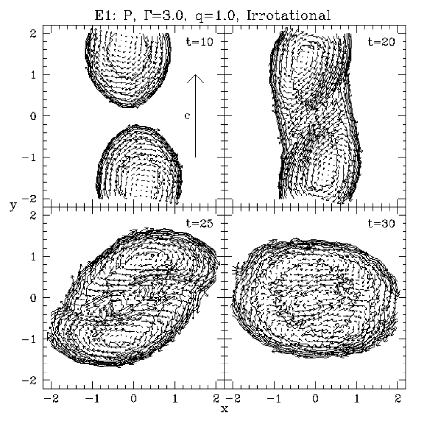
FIG. 2.: Density contours in the orbital plane and velocity field shown in the corotating frame for the evolution in run E1 ($\Gamma=3$, q=1). The physical speed of light, $c_{2.5PN}=2.5$, is shown to indicate the scale. Upon first contact of the NS, two counterstreaming layers form a turbulent vortex sheet. As the cores of the respective NS continue to inspiral, we see the formation of a merger remnant with the beginnings of a more coherent differential rotation pattern.

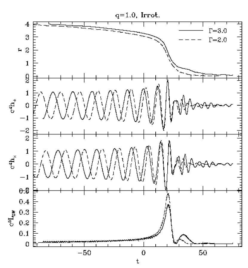
FIG. 3.: Binary separation (top panel), GW amplitudes in both polarizations (middle panels) and GW luminosity (bottom panel) as a function of time for runs E1 and F1. The solid lines correspond to run E1 ($\Gamma=3$), the dashed lines to run F2 ($\Gamma=2$). The dynamical stability limit for the softer EOS lies within that of the stiffer one. The softer EOS also results in a higher peak GW luminosity, but smaller amplitude post-merger GW emission.

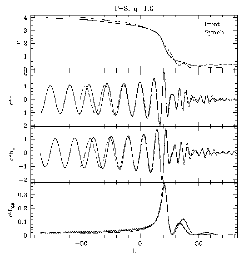
FIG. 4.: Binary separation (top panel), GW amplitudes (middle panels) and GW luminosity (bottom panel) as a function of time for runs E1 and B1, started from an irrotational (solid line) and a synchronized (dashed line) initial condition, respectively. The synchronized run contains more energy and is relatively more dynamically unstable. While the initial peaks in the GW luminosities are of similar amplitude, the secondary peaks are much more luminous for the synchronized binary.

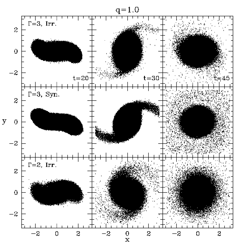
FIG. 5.: Particle plots for runs E1 ($\Gamma=3$; top panels), B1 (synchronized, $\Gamma=3$; middle panels), and F1 ($\Gamma=2$; bottom panels), described in Figs. 3 and 4. The orbital rotation is in the counter-clockwise direction. The plots show projections of all SPH particles at $t=20$ (left), $t=30$ (center), and $t=45$ (right). Mass shedding is more sensitively dependent on the initial velocity field, but the remnant equatorial ellipticity, and thus the post-merger GW emission, is dominated by the choice of EOS.

FIG. 6.: Angular velocity as a function of cylindrical radius (top panel) and enclosed mass as a function of radius for the remnants of runs B1, E1, and F1, described in Figs. 3 and 4. The profiles, all taken at $t=65$, correspond to irrotational run E1 ($\Gamma=3$; solid line), run F1 ($\Gamma=2$; dashed line), and run B1 (synchronized, $\Gamma=3$; dotted line).

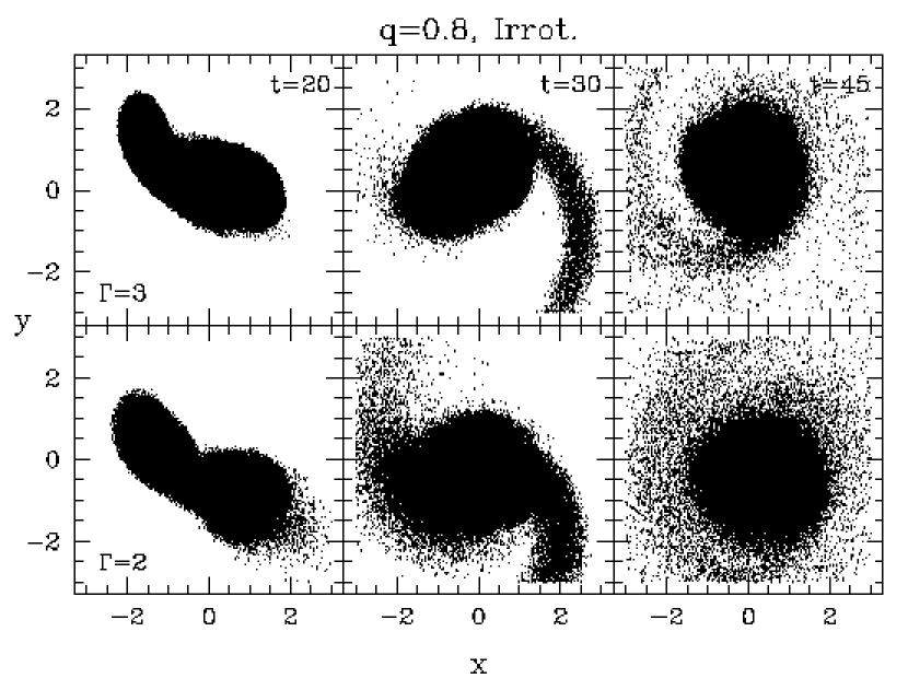
FIG. 7.: Particle plots for runs E2 ($q=0.8$, $\Gamma=3$; top panels) and F2 ($q=0.8$, $\Gamma=2$; bottom panels), respectively. From left to right, we see snapshots taken at $t=20$, $t=30$, and $t=45$, showing in both cases the tidal disruption of the secondary, the formation of a single spiral arm during mass shedding, and the eventual creation of a massive torus around the merger remnant.

FIG. 8.: Binary separation (top panel), GW amplitudes (middle panels) and GW luminosity (bottom panel) as a function of time for our irrotational runs E2 and F2, as shown in Fig. 7. The solid and dashed curves correspond to run E2 ($\Gamma=3$) and run F2 ($\Gamma=2$), respectively. We see that GW production is significantly suppressed for the softer $\Gamma=2$ EOS during the first peak.

FIG. 9.: Binary separation (top panel) and the ratio of each star’s spin angular momentum to its total angular momentum (bottom panel) as a function of time for runs E1 and T2 which started from an initial separation $r_{0}=4.0$ (solid line) and $r_{0}=3.5$ (dashed line), respectively. The binary with larger initial separation develops greater spin angular momentum throughout the calculation prior to merger.

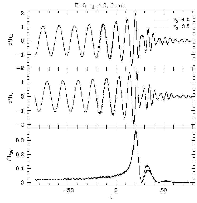
FIG. 10.: GW amplitudes in both polarizations (top and middle panel) and GW luminosities (bottom panel) for the two runs described in Fig. 9. The agreement is excellent throughout, except for a slight difference in the amplitude of the second GW peak.

FIG. 11.: Angular velocity as a function of cylindrical radius (top panel) and enclosed mass as a function of radius for the remnants of the runs shown in Fig. 9. The profiles are taken at $t=65$ for both runs. We see that mass shedding to larger radii is very slightly increased for the calculation started from $r_{0}=4.0$, but that in both cases virtually all the matter in the system ends up in the remnant itself. The inset shows the profile at the outer edge of the system, indicating that no more than $\simeq 0.5\%$ of the material is ejected to larger radii.

FIG. 12.: GW luminosities (top) and waveforms (middle and bottom) for calculations using increasing number of particles. The dotted lines correspond to run T1 ($N=10^{4}$), the solid lines to run T2 ($N=10^{5}$), and the dashed lines to run T3 ($N=10^{6}$). We see that the two highest resolution runs agree almost perfectly. The lowest resolution run is more susceptible to initial deviations from equilibrium, and shows some significant differences from the higher resolution runs, especially after the first GW luminosity peak.

FIG. 13.: Density contours in the orbital plane and velocity field in the corotating frame of the binary at $t=20$ for runs T1, T2, and T3, shown in Fig. 12. We see some discrepancies in the extent of vortex formation between the lowest resolution run and the two higher resolution runs, which agree well.

FIG. 14.: Density contours in the orbital plane and velocity field in the corotating frame of the binary at $t=25$ for the runs shown in Fig. 13, with the same conventions as in that figure. We see that matter between the large vortices is directed toward the center of the remnant in the two lower resolution runs, whereas the flow lines are straighter along the vortex sheet in the highest resolution run.

FIG. 15.: Energy spectrum in GW calculated using Eq. 14 from a typical Newtonian calculation (synchronized, $q=1$, $\Gamma=3$). We show the inspiral (dotted line) and merger (dashed line) subcomponents of the spectrum, as well as the total combined spectrum (heavy solid line).

FIG. 16.: Energy spectrum from a typical PN calculation, run E1 ($q=1.0$, $\Gamma=3$). Conventions are as in Fig. 15. We see that the energy emitted during the late stages of inspiral is greatly suppressed relative to the Newtonian case. The two prominent peaks at higher frequencies correspond to the maximum GW luminosity and final merger remnant oscillation.

FIG. 17.: Comparison of GW energy spectra calculated from runs which differ in initial separation (top panel) or numerical resolution (bottom panel). In the top panel, we show the spectra for runs E1 and T2, started from $r_{0}=4.0$ (thin solid line) and $r_{0}/R=3.5$ (thick solid line), respectively. In the bottom panel, we show the spectra from runs T1 and T2 with $N=10^{4}$ (thin solid line) and $N=10^{5}$ (thick solid line), respectively.

FIG. 18.: Comparison of GW energy spectra from runs which differ in the choice of EOS (top panel) and initial velocity profile (bottom panel) for equal mass NS. In the top panel, we show the spectra for runs E1 and F1, with a $\Gamma=3$ EOS (thin solid line) and a $\Gamma=2$ EOS (thick solid line), respectively. In the bottom panel we show the comparison between run E1 and run B1 (with a synchronized initial condition; thick solid line).

FIG. 19.: Comparison of GW energy spectra for binaries with different mass ratios and NS with a $\Gamma=3$ (top panel) or $\Gamma=2$ (bottom panel) EOS. Thin solid lines represent the spectra for equal-mass runs T2 and F1, thick solid lines for runs E2 and F2 with $q=0.8$. Binaries with $q<1$ not only have lower amplitude through the lower frequency portion of the spectrum, but also lack clear peaks at the characteristic frequency of maximum GW emission.

TABLE I.: Input parameters for the runs described in this paper: $\Gamma$ is the adiabatic exponent, $q$ the binary mass ratio, and $r_{0}$ the initial separation. All runs used $10^{5}$ SPH particles, except testing runs T1 and T3, with $10^{4}$ and $10^{6}$ SPH particles, respectively. Testing run T2 differs from run E1 only in the initial separation. All runs in this paper were started from an irrotational initial condition.

Run	$\Gamma$	$q$	$r_{0}$	$\log_{10}N$
E1	3.0	1.00	4.0	5
E2	3.0	0.80	3.5	5
F1	2.0	1.00	4.0	5
F2	2.0	0.80	3.5	5
T1	3.0	1.00	3.5	4
T2	3.0	1.00	3.5	5
T3	3.0	1.00	3.5	6

TABLE II.: Selected results from each run. Here, $t_{0}$ is the time at which the run was started, and $\theta_{\rm lag}$ is the lag angle at first contact, given for the primary and secondary, respectively, for systems with $q\neq 1.0$. Quantities involving the first and second GW luminosity peaks are labeled with superscripts $(1)$ and $(2)$.

Run	$t_{0}$	$\theta_{lag}(deg)$	$L_{\rm max}^{(1)}$	$h_{\rm max}^{(1)}$	$L_{\rm max}^{(2)}$	$h_{\rm max}^{(2)}$	$t^{(2)}$
E1	-86	7.5	0.374	2.023	0.093	0.807	33
E2	-39	6.5, 8.4	0.156	1.524	0.045	0.602	35
F1	-105	10.0	0.479	2.129	0.050	0.545	30
F2	-55	3.8, 12.1	0.098	1.364	0.056	0.564	35
T1	-21	7.8	0.358	2.009	0.125	0.932	32
T2	-3	12.0	0.337	1.972	0.087	0.746	30
T3	-16	5.8	0.356	1.989	0.111	0.907	32

TABLE III.: Properties of the merger remnants. Here $M_{r}$ is the rest mass of the remnant, $M_{gr}$ is its gravitational mass, $a_{r}$ is its Kerr parameter, $\Omega_{c}$ and $\Omega_{eq}$ are the angular rotation velocities at the center and at the equator, and the $a_{i}$’s and $I_{i}$’s are the radii of the principal axes and moments of inertia.

run	$M_{r}$	$M_{gr}$	$a_{r}$	$\Omega_{c}$	$\Omega_{eq}$	$a_{1}$	$a_{2}/a_{1}$	$a_{3}/a_{1}$	$I_{2}/I_{1}$
E1	1.95	1.88	0.73	0.668	0.435	1.81	0.94	0.55	1.07
F1	1.94	1.79	0.81	0.838	0.436	1.83	0.96	0.49	1.01
T1	1.97	1.91	0.74	0.711	0.433	1.81	0.94	0.54	1.10
T2	1.97	1.91	0.74	0.735	0.414	1.80	0.98	0.57	1.07

TABLE IV.: GW quantities computed for runs with different numbers of particles $N$ at representative times. Here, $h(t)$ is the GW strain, and $\Omega_{GW}(t)$ is the instantaneous angular frequency of the GWs. At $t=10$, the stars are about to make contact, $t=20$ is the moment of peak GW luminosity, and by $t=30$ a remnant has begun to form. In all cases, we see much better agreement between the two higher resolution runs, at a level of $\simeq 2\%$.

run	N	$h(t=10)$	$\Omega_{GW}(t=10)$	$h(t=20)$	$\Omega_{GW}(t=20)$	$h(t=30)$	$\Omega_{GW}(t=30)$
T1	$10^{4}$	1.49	0.556	1.71	1.053	0.74	1.192
T2	$10^{5}$	1.57	0.584	1.91	0.978	0.90	1.166
T3	$10^{6}$	1.58	0.581	1.87	0.996	0.89	1.154