On the spinning C-metric

Abstract

Physical interpretation of some stationary and non-stationary regions of the spinning C-metric is presented. They represent different spacetime regions of a uniformly accelerated Kerr black hole. Stability of geodesics corresponding to equilibrium points in a general stationary spacetime with an additional symmetry is also studied and results are then applied to the spinning C-metric.

I Introduction

The C-metric is a well known exact Petrov type D vacuum solution of Einstein’s field equations found in the second decade of the last centurylevi ; weyl . However, it was much later when its physical interpretation was foundKinnWalker ; BonnorN . Its most physical region represents a pair of Schwarzschild black holes connected by a conical singularity and uniformly accelerated in opposite directions along the axis of axial symmetry.

The C-metric is an example of boost-rotation symmetric spacetimesBicSchPRD ; JibiEhlers ; AVrev corresponding to gravitational field of uniformly accelerated “particles” of various kinds. Thus for the physical interpretation it is worthwhile to express the C-metric in coordinates adapted to the boost and rotation symmetriesBonnorN .

Several generalizations of the C-metric (e.g., for charged black holesKinnWalker ; Cornish-el , for an external field presenternst or recently for two or more black holes accelerated in both directions along the axis of symmetryDowker ) were found. Probably the most important of them is the spinning C-metric (the SC-metric) found by Plebański and DemiańskiPlebDem , which is also of the Petrov type D. In the present paper, we restrict ourselves to the case with non-vanishing mass, angular momentum, and acceleration and we set electric and magnetic charges, the NUT parameter, and the cosmological constant equal to zero. Then the SC-metric in coordinates adapted to its special algebraical structure reads

$${\rm d}s^{2}=\frac{1}{H^{\prime}}\Bigl{[}\frac{W^{\prime}}{P}{\rm d}p^{2}+\frac{P}{W^{\prime}}\left({\rm d}\sigma+q^{2}{\rm d}\tau^{\prime}\right)^{2}+\frac{W^{\prime}}{Q}{\rm d}q^{2}-\frac{Q}{W^{\prime}}\left({\rm d}\tau^{\prime}-p^{2}{\rm d}\sigma\right)^{2}\Bigr{]}\ ,$$ (1)

where

$$P = \ \ \gamma^{\prime}-{\varepsilon^{\prime}}\,{p}^{2}+2\,m^{\prime}{p}^{3}-\gamma^{\prime}{p}^{4}\ ,$$

$$Q = -\gamma^{\prime}+{\varepsilon^{\prime}}\,{q}^{2}+2\,m^{\prime}{q}^{3}+\gamma^{\prime}{q}^{4}\ ,$$

$$H^{\prime} = (p+q)^{2}\ ,$$

$$W^{\prime} = \ 1+(pq)^{2}\$$

with $\gamma^{\prime}$, $\varepsilon^{\prime}$, and $m^{\prime}$ being constant.

By performing certain limiting proceduresPlebDem that remove the acceleration or rotation parameters one obtains the Kerr solution or the C-metric, respectively.

Physical properties of the SC-metric were studied in FZ ; bivoj ; Letelier . Stationary regions of the SC-metric (1) and Killing horizons were identified in bivoj . Then the most physical stationary region was transformed into the Weyl-Papapetrou coordinates and finally to coordinates adapted to the boost and rotation symmetries. The SC-metric is the only example of boost-rotation symmetric spacetimes with spinning sourcesav-brs known today.

In the present paper, we start with the SC-metric in a better chosen parametrization than in (1) that makes the physical interpretation more transparent. As in bivoj , we first transform stationary regions of the SC-metric to the Weyl-Papapetrou form (Sec. III) and then to coordinates adapted to the boost and rotation symmetries (Sec. IV), where non-stationary radiative regions appear. It is shown that these non-stationary regions (inside and outside the null cone of the origin) are in fact already contained in the original form of the SC-metric. This also enables us to locate ${\cal J^{+}}$ and $I^{+}$.

It is shown in bivoj that the most physical stationary region $\cal{B}$ corresponds to a field of a uniformly accelerated Kerr black hole. Here, another stationary region is interpreted as a uniformly accelerated white hole with a ring singularity that in fact corresponds to the uniformly accelerated asymptotically flat “interior” of the Kerr solution.

In Sec. V, geodesics and their stability are studied at first generally for an arbitrary stationary metric with another symmetry and then results are applied to the stationary region ${\cal B}$ of the SC-metric.

II The spinning C-metric in the $\{\tau$, $x$, $y$, $\phi\}$ coordinates

Since the parameters $\gamma^{\prime}$ and $\varepsilon^{\prime}$ occurring in (1) do not have a straightforward connection with the angular momentum and acceleration of the black hole, we start with the SC-metric with rescaled parameters and coordinatesLetelier

$${\rm d}s^{2}=\frac{1}{H}\left[\frac{W}{F}{\rm d}y^{2}+\frac{W}{G}{\rm d}x^{2}+\frac{G}{W}({\rm d}\phi+aAy^{2}{\rm d}\tau)^{2}-\frac{F}{W}({\rm d}\tau-aAx^{2}{\rm d}\phi)^{2}\right]\ ,$$ (2)

where

$$F = -\delta-\varepsilon y^{2}-2mAy^{3}+(aA)^{2}\delta y^{4}\ ,$$

$$G = \delta+\varepsilon x^{2}-2mAx^{3}-(aA)^{2}\delta x^{4}\ ,$$

$$H = A^{2}(x+y)^{2}\ ,$$

$$W = 1+(aAxy)^{2}\$$

with $m$, $a$, $A$, $\delta$, and $\varepsilon$ being constant. The metrics (1) and (2) are related by the trivial transformation

$$p=\sqrt{aA}\ x\ ,\mbox{\quad}q=\sqrt{aA}\ y\ ,\mbox{\quad}\sigma=\sqrt{\frac{a}{A^{3}}}\ \phi\ ,\mbox{\quad}\tau^{\prime}=\sqrt{\frac{a}{A^{3}}}\ \tau\ ,$$

$$\gamma^{\prime}=A^{2}\delta\ ,\mbox{\quad}\varepsilon^{\prime}=-\frac{A\varepsilon}{a}\ ,\mbox{\quad}m^{\prime}=-m\sqrt{\frac{A^{3}}{a^{3}}}\ .\mbox{\quad}\mbox{\quad}\mbox{\quad}\mbox{\quad}$$

Notice that for

$$\delta=1\ ,\mbox{\quad}\varepsilon=-1\ ,$$ (3)

and $a=0$ we get the standard form of the non-spinning C-metric. In the following, we assign the foregoing values (3) to the kinematical parameters $\delta$ and $\varepsilon$.

In the present paper, we study only the case when the polynomial $F=-1+y^{2}-2mAy^{3}+(aA)^{2}y^{4}$ has four distinct real roots $y_{1}\ ,\dots,\ y_{4}$. This is satisfied if the conditions

$$m^{2}>\frac{8}{9}\ a^{2}\mbox{\quad}\mbox{and}\mbox{\quad}\alpha_{1}-\alpha_{2}<A^{2}<\alpha_{1}+\alpha_{2}\ ,$$ (4)

where

$$\alpha_{1}=\frac{1}{32a^{6}}\left(36\,{a}^{2}{m}^{2}-8\,{a}^{4}-27\,{m}^{4}\right)\ ,\mbox{\quad}\alpha_{2}=\frac{m}{32a^{6}}\left(9\,{m}^{2}-8\,{a}^{2}\right)^{3/2}\ ,$$

hold. Notice that ${\alpha_{1}}^{2}-{\alpha_{2}}^{2}=(a^{2}-m^{2})/(16a^{2})$. For $m^{2}>a^{2}$, $\alpha_{1}-\alpha_{2}$ is negative and then $A^{2}$ has to fulfil only the upper constraint. In the limit $a\rightarrow 0$, the upper constraint for $A^{2}$, $\alpha_{1}+\alpha_{2}$, turns out to be $1/(27m^{2})$, which is the same as for the non-spinning C-metric. If $y_{i}$ are the roots of $F$ then $-y_{i}$ are the roots of $G$ since $F(y)=-G(-y)$.

Similarly as in bivoj , it can be shown that the metric (2) has the signature $+2$ for $G>0$ and is then stationary for $F>0$. In the coordinates $\{\tau$, $x$, $y$, $\phi\}$, there are four stationary regions (see Fig. 1) ${\cal A}$, ${\cal B}$, ${\cal C}\cup{\cal C}^{\prime}$, and ${\cal D}\cup{\cal D}^{\prime}$ (as in bivoj , we identify $y=\infty$ and $y=-\infty$) and each of them can be transformed to the stationary Weyl-Papapetrou form (see Sec. III).

Curvature invariants

$$R^{\alpha\beta\gamma\delta}R_{\alpha\beta\gamma\delta} = 48m^{2}\frac{H^{3}}{W^{6}}(W-2)(W^{2}-16W+16)\ ,$$ (5)

$${{\scriptstyle{\frac{1}{2}}}}\epsilon^{\alpha\beta\sigma\rho}{R_{\sigma\rho}}^{\mu\nu}R_{\alpha\beta\mu\nu} = 96aAm^{2}xy\frac{H^{3}}{W^{6}}(3W-4)(W-4)\$$ (6)

suggest that there are curvature singularities at points $(x=0$, $y=\pm\infty)$ and $(x=\pm\infty$, $y=0)$. The second curvature invariant also indicates that the constant $a$ is proportional to the angular momentum of the source Ciuf . Both invariants vanish for $x+y=0$. Later it will be shown that ${\cal J}^{+}$, $I^{+}$, and $I^{0}$ are located there (see Fig. 4).

Killing horizons, which are located at $y=y_{i}$, correspond to the black hole or acceleration horizons bivoj (see Fig. 1).

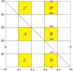
Figure 1: The structure of the SC-metric (2) in the coordinates $\{\tau$, $x$, $y$, $\phi\}$: The metric has the signature $+2$ for $G>0$, i.e., in the second and fourth columns from the left, and is stationary for $F>0$ in the shaded squares. Curvature singularities at points $(x=0$, $y=\pm\infty)$ and $(x=\pm\infty$, $y=0)$ are denoted by crosses. The black hole horizons and the acceleration horizons are labeled by BH and AH, respectively. The line $x+y=0$, where curvature invariants (5) and (6) vanish, is also indicated.

III Transformation to the Weyl-Papapetrou coordinates

As was mentioned earlier, each of the four stationary regions ${\cal A}$, ${\cal B}$, ${\cal C}\cup{\cal C}^{\prime}$, and ${\cal D}\cup{\cal D}^{\prime}$ can be transformed to the stationary Weyl-Papapetrou coordinates $\{{\bar{t}}$, ${\bar{\rho}}$, ${\bar{z}}$, ${\bar{\varphi}}\}$

$${\rm d}s^{2}={\rm e}^{-2U}[{\rm e}^{2\nu}({\rm d}{\bar{\rho}}^{2}+{\rm d}{\bar{z}}^{2})+{\bar{\rho}}^{2}{\rm d}{\bar{\varphi}}^{2}]-{\rm e}^{2U}({\rm d}{\bar{t}}+{\bar{\omega}}{\rm d}{\bar{\varphi}})^{2}\ ,$$ (7)

where the metric functions $U$, $\nu$, and ${\bar{\omega}}$ are functions of ${\bar{\rho}}$ and ${\bar{z}}$. The transformation

$$\bar{\rho}^{2} = {\cal K}^{2}FGH^{-2}\ ,$$ (8)

$$\bar{z} = {\cal K}[1+mAxy(x-y)+xy-a^{2}A^{2}x^{2}y^{2}]H^{-1}\ ,$$ (9)

$$\tau = \kappa_{1}\bar{t}+\kappa_{2}\bar{\varphi}\ ,$$ (10)

$$\phi = \kappa_{3}\bar{t}+\kappa_{4}\bar{\varphi}\ ,$$ (11)

$${\cal K} = \kappa_{2}\kappa_{3}-\kappa_{1}\kappa_{4}\ ,$$ (12)

where $\kappa_{1}\dots\kappa_{4}$ are constant, can be found similarly as in bivoj . It turns out that it is convenient to choose

$${\cal K}=A$$ (13)

since then the SC-metric in the Weyl-Papapetrou coordinates with appropriately chosen constants $\kappa_{1}\dots\kappa_{4}$ yields the Kerr solution in the limit $A\rightarrow 0$. In the following, we assume that (13) holds.

In the present paper, $\tau$, $x$, $y$, $\phi$, ${\bar{\varphi}}$, $\kappa_{2}$, and $\kappa_{4}$ are dimensionless and ${\bar{t}}$, ${\bar{\rho}}$, ${\bar{z}}$, $m$, $a$, $1/A$, $1/\kappa_{1}$, and $1/\kappa_{3}$ have the dimension of length.

In order to express the SC-metric in the Weyl-Papapetrou form (7) we have to find the inverse transformation to (8), (9). Let us first define $R_{i}$

$$R_{i}\equiv\sqrt{\bar{\rho}^{2}+(\bar{z}-\bar{z}_{i})^{2}}\ ,\mbox{\quad}i=1\dots 3\ ,$$ (14)

where ${\bar{z}}_{i}$ are the roots of the cubic equation

$$2A{\bar{z}}_{i}^{3}-{\bar{z}}_{i}^{2}+2Aa^{2}{\bar{z}}_{i}+m^{2}-a^{2}=0\ .$$ (15)

It can be shown that

$${R_{i}}^{2}=\frac{\left(\frac{A_{i}}{A\bar{z}_{i}}+\frac{A^{2}m\bar{z}_{i}}{A_{i}}(x-y)-A_{i}xy\right)^{2}}{A^{2}(x+y)^{2}}\ ,$$

where

$$A_{i}^{2}=A^{2}(2Aa^{2}\bar{z}_{i}+m^{2}-a^{2})\ .$$

Then

$$R_{i}=\epsilon_{i}\frac{\left(\frac{A_{i}}{A\bar{z}_{i}}+\frac{A^{2}m\bar{z}_{i}}{A_{i}}(x-y)-A_{i}xy\right)}{A(x+y)}\ ,$$ (16)

where $\epsilon_{i}=\pm 1$. Each of the stationary regions is characterized by a different combination of $\epsilon_{i}$:

${\cal A}:\mbox{\quad}$	$\epsilon_{1}=-1\ ,$	$\epsilon_{2}=-1\ ,$	$\epsilon_{3}=+1\ ,$
${\cal B}:\mbox{\quad}$	$\epsilon_{1}=-1\ ,$	$\epsilon_{2}=+1\ ,$	$\epsilon_{3}=-1\ ,$
${\cal C}\cup{\cal C}^{\prime}:\mbox{\quad}$	$\epsilon_{1}=+1\ ,$	$\epsilon_{2}=+1\ ,$	$\epsilon_{3}=+1\ ,$
${\cal D}\cup{\cal D}^{\prime}:\mbox{\quad}$	$\epsilon_{1}=+1\ ,$	$\epsilon_{2}=-1\ ,$	$\epsilon_{3}=-1\ .$

Now solving Eqs. (16) for $x$ and $y$, the inverse transformation can be found

$$x=\frac{F_{0}+F_{1}}{F_{2}}\ ,\quad y=\frac{F_{0}-F_{1}}{F_{2}}\ ,$$ (17)

where

$$F_{0} = \epsilon_{1}\epsilon_{2}\epsilon_{3}(m^{2}-a^{2})A^{2}({\bar{z}}_{1}-{\bar{z}}_{2})({\bar{z}}_{2}-{\bar{z}}_{3})({\bar{z}}_{3}-{\bar{z}}_{1})\ ,$$

$$F_{1} = {\bar{z}}_{1}A_{2}A_{3}\epsilon_{3}\epsilon_{2}({\bar{z}}_{3}-{\bar{z}}_{2})R_{1}+A_{1}{\bar{z}}_{2}A_{3}\epsilon_{1}\epsilon_{3}({\bar{z}}_{1}-{\bar{z}}_{3})R_{2}+A_{1}A_{2}{\bar{z}}_{3}\epsilon_{2}\epsilon_{1}({\bar{z}}_{2}-{\bar{z}}_{1})R_{3}\ ,$$

$$F_{2} = (m^{2}-a^{2})A\left[\epsilon_{2}\epsilon_{3}({\bar{z}}_{2}-{\bar{z}}_{3})A_{1}R_{1}+\epsilon_{3}\epsilon_{1}({\bar{z}}_{3}-{\bar{z}}_{1})A_{2}R_{2}+\epsilon_{1}\epsilon_{2}({\bar{z}}_{1}-{\bar{z}}_{2})A_{3}R_{3}\right]\ .$$

From the transformation (8)–(12) follows

$$g_{{\bar{\rho}}{\bar{\rho}}} = \frac{W}{HF({{\bar{\rho}},_{y}}^{2}+{{\bar{z}},_{y}}^{2})}\ ,$$

$$g_{\bar{t}\bar{t}} = \frac{-\left({\it\kappa_{1}}-a{x}^{2}{\it\kappa_{3}}\,A\right)^{2}F+\left({\it\kappa_{3}}+a{y}^{2}{\it\kappa_{1}}\,A\right)^{2}G}{HW}\ ,$$

$$g_{\bar{\varphi}\bar{\varphi}} = \frac{\left({\it\kappa_{2}}-a{x}^{2}{\it\kappa_{4}}\,A\right)^{2}F-\left({\it\kappa_{4}}+a{y}^{2}{\it\kappa_{2}}\,A\right)^{2}G}{HW}\ ,$$ (18)

$$g_{\bar{t}\bar{\varphi}} = \frac{-\left({\it\kappa_{2}}-a{x}^{2}{\it\kappa_{4}}\,A\right)\left({\it\kappa_{1}}-a{x}^{2}{\it\kappa_{3}}\,A\right)F+\left({\it\kappa_{4}}+a{y}^{2}{\it\kappa_{2}}\,A\right)\left({\it\kappa_{3}}+a{y}^{2}{\it\kappa_{1}}\,A\right)G}{HW}$$

with $x$ and $y$ given by (17). The Weyl-Papapetrou metric functions are now

$${\rm e}^{2U}=-g_{\bar{t}\bar{t}}\ ,\mbox{\quad}{\rm e}^{2\nu}=-g_{{\bar{\rho}}{\bar{\rho}}}g_{\bar{t}\bar{t}}\ ,\mbox{\quad}{\bar{\omega}}=g_{\bar{t}\bar{\varphi}}/g_{\bar{t}\bar{t}}\ .$$ (19)

Substituting Eqs. (17) and (18) into (19) we obtain the SC-metric in the Weyl-Papapetrou coordinates. Unfortunately, these expressions are very complicated and can be handled only by computer manipulations. In the non-spinning case, our approach gives again long formulas, whereas GodfreyGodfrey and BonnorBonnorN , after performing very long calculations, arrived at considerably simpler equivalent results. A similar simplification may be probably also possible in the spinning case. The spinning soliton generalizationLetelsolit of the non-spinning C-metric might be helpful in this task.

The regularity condition on the axis reads

$${\lim_{{\bar{\rho}}_{0}\rightarrow 0}\frac{1}{2\pi}\frac{\int_{0}^{2\pi}\sqrt{g_{{\bar{\varphi}}{\bar{\varphi}}}({\bar{\rho}}_{0},{\bar{z}})}{\rm d}{\bar{\varphi}}}{\int_{0}^{{\bar{\rho}}_{0}}\sqrt{g_{{\bar{\rho}}{\bar{\rho}}}({\bar{\rho}},{\bar{z}})}{\rm d}{\bar{\rho}}}=1}\ ,$$

from which follows

$$\nu = 0\ ,$$ (20)

$${\bar{\omega}} = 0\$$ (21)

on the axis. When both conditions (20) and (21) are satisfied then the axis is regular. If only (21) holds then there is a conical singularity (a string or a strut); if none of these conditions is satisfied a spinning string (conical and torsionletolstring ; bonnor singularity) is present and, in its vicinity, a region with closed timelike curves occurs. Vacuum Einstein’s equations allow us to multiply ${\rm e}^{2\nu}$ by a constant $\kappa_{5}$. Later we will adjust this constant to regularize some parts of the axis.

Let us now restrict ourselves to the most physically interesting stationary region ${\cal B}$ of the SC-metric (2), which was studied in the non-spinning and spinning cases in papers BonnorN ; cornish ; AVrev ; Letelier and bivoj ; Letelier , respectively.

In the Weyl-Papapetrou form, the black hole horizon is located on the axis between ${\bar{z}}_{1}$ and ${\bar{z}}_{2}$, the acceleration horizon extends from ${\bar{z}}_{3}$ to $\infty$, and there may occur conical singularities or spinning strings on the rest of the axis depending on the values of the constants $\kappa_{1}\dots\kappa_{5}$ (see Fig. 2 a).

Let us now fix the appropriate values of the constants $\kappa_{1}\dots\kappa_{5}$:

Requiring $g_{\bar{t}\bar{\varphi}}=0$ and $g_{\bar{\varphi}\bar{\varphi}}\not=0$ on the acceleration horizon (where $y=y_{2}$, $F=0$) leads to the condition

$$\kappa_{3}+ay_{2}^{2}A\kappa_{1}=0\ .$$ (22)

Demanding further that there be no torsion singularity on the axis for ${\bar{z}}<\bar{z}_{1}$ (where $G=0$, $x=x_{3}=-y_{2}$), i.e., ${\bar{\omega}}$ and thus also $g_{\bar{t}\bar{\varphi}}$ vanish there (21), we arrive at

$$\kappa_{2}-ay_{2}^{2}A\kappa_{4}=0\ .$$ (23)

Equivalent conditions were obtained in bivoj requiring the appropriate asymptotical behaviour of the metric in the coordinates adapted to the boost and rotation symmetries discussed in Sec. IV.

From Eqs. (13), (22), and (23) we obtain

$$\kappa_{4}=-\frac{A}{\kappa_{1}(1+a^{2}A^{2}{y_{2}}^{4})}\ .$$ (24)

Further requirement on the axis – to be regular for ${\bar{z}}<\bar{z}_{1}$ (20) – leads to

$$\kappa_{5}=-\frac{A^{2}(-1+4y_{2}(mA-a^{2}A^{2}y_{2})+(a^{2}-m^{2})A^{2}{y_{2}}^{4})}{{\kappa_{1}}^{2}(1+a^{2}A^{2}{y_{2}}^{4})^{2}}\ .$$ (25)

By Eqs. (22)–(25) together with Eq. (30) the constants $\kappa_{1}\dots\kappa_{5}$ are uniquely determined.

The “angular velocity” of the black hole horizon $y=y_{3}$ turns out to be

$$\Omega_{H}\equiv-\frac{g_{{\bar{t}}{\bar{t}}}}{g_{{\bar{t}}{\bar{\varphi}}}}_{|y=y_{3}}=\frac{aA^{2}({y_{3}}^{2}-{y_{2}}^{2})}{1+(aAy_{2}y_{3})^{2}}\ ,$$ (26)

where Eqs. (18), (22)–(24), and (30) were employed. Notice that the expression (26) differs from $\Omega_{H}$ of Letelier and Oliveira Letelier since we use a different coordinate system that does not rotate asymptotically.

For $a<m$ and the acceleration $A\rightarrow 0$, Eq. (26) reduces to

$$\lim_{A\rightarrow 0}\Omega_{H}=\frac{a}{2m(m+\sqrt{m^{2}-a^{2}})}\$$

that is equal to $\Omega_{H}$ for the outer horizon of the Kerr metric.

For $a<m$ and $A<<1$, the roots of (15) are

$${\bar{z}_{1}} = -\sqrt{m^{2}-a^{2}}+m^{2}A+{\cal O}(A^{2})\ ,$$

$${\bar{z}_{2}} = \sqrt{m^{2}-a^{2}}+m^{2}A+{\cal O}(A^{2})\ ,$$

$${\bar{z}_{3}} = \frac{1}{2A}-2m^{2}A+{\cal O}(A^{2})\ .$$

In the limit $A\rightarrow 0$, there remains only the black hole horizon on the axis between $-\sqrt{m^{2}-a^{2}}$ and $+\sqrt{m^{2}-a^{2}}$ since ${\bar{z}_{3}}\rightarrow\infty$. This indicates that in this limit the SC-metric in the Weyl-Papapetrou coordinates with the appropriate choice of $\kappa_{1}\dots\kappa_{5}$ approaches the Kerr solution. Indeed, the metric functions ${\rm e}^{2U}$, ${\rm e}^{2\nu}$, and ${\bar{\omega}}$ with $\kappa_{1}\dots\kappa_{5}$ given by (22)–(25) and (30) go to the corresponding metric functions of the Kerr metric in the Weyl-Papapetrou coordinates as given, e.g., in kramer .

In this section, we have transformed the region ${\cal B}$ of the SC-metric into the Weyl-Papapetrou coordinates. It is similarly possible to transform the region ${\cal D}\cup{\cal D}^{\prime}$ there, however, another choice of the constants $\kappa_{1}\dots\kappa_{5}$ would be appropriate in Eqs. (8)–(12). The white hole horizon appears on the axis between ${\bar{z}}_{1}$ and ${\bar{z}}_{2}$ and the acceleration horizon for ${\bar{z}}>{\bar{z}}_{3}$. Moreover there is a ring singularity at ${\bar{z}}=0$ and ${\bar{\rho}}=a$ (corresponding to $x=0$ and $y=\pm\infty$), where curvature invariants go to infinity. For the limit $A\rightarrow 0$ we obtain the region $r\in(-\infty,\ r_{-})$ of the Kerr spacetime, where $r$ is the Boyer-Lindquist coordinate. The region ${\cal D}\cup{\cal D}^{\prime}$ thus corresponds to the spacetime of a uniformly accelerated white hole with a ring singularity.

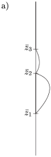
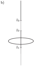
Figure 2: a) The ${\cal B}$ region of the SC-metric in the Weyl-Papapetrou coordinates: The black hole and acceleration horizons are located on the axis ${\bar{\rho}}=0$ at ${\bar{z}}\in$ $({\bar{z}}_{1},\ {\bar{z}}_{2})$ and at ${\bar{z}}\in$ $({\bar{z}}_{3},\ \infty)$, respectively. There is an ergoregion in the vicinity of the black hole horizon and a region with closed timelike curves in the neighbourhood of the spinning string between ${\bar{z}}_{2}$ and ${\bar{z}}_{3}$.
b) The ${\cal D}\cup{\cal D}^{\prime}$ region of the SC-metric in the Weyl-Papapetrou coordinates: The white hole and acceleration horizons are located on the axis at ${\bar{z}}\in$ $({\bar{z}}_{1},\ {\bar{z}}_{2})$ and ${\bar{z}}\in$ $({\bar{z}}_{3},\ \infty)$, respectively. The ring singularity with the radius ${\bar{\rho}}=a$ appears at ${\bar{z}}=0$.

IV The spinning C-metric in the coordinates adapted to the boost and rotation symmetries

Now let us transform the region ${\cal B}$ into the coordinates adapted to the boost and rotation symmetries $\{t$, $\rho$, $z$, $\varphi\}$. The transformation BS ; BonnorN

$${\bar{\rho}}^{2} = A^{2}\rho^{2}(z^{2}-t^{2})\ ,$$

$${\bar{\varphi}} = \varphi\ ,$$ (27)

$${\bar{z}}-{\bar{z}}_{3} = {{\scriptstyle{\frac{1}{2}}}}A(\rho^{2}+t^{2}-z^{2})\ ,$$

$${\bar{t}} = \frac{1}{A}{\rm arctanh}\left(\frac{t}{z}\right)\$$

leads to the metric of boost-rotation symmetric spacetimes with spinning sourcesbivoj ; av-brs

$${\rm d}s^{2} = {\rm e}^{\lambda}{\rm d}\rho^{2}+\rho^{2}{\rm e}^{-\mu}{\rm d}\varphi^{2}-2\omega{\rm e}^{\mu}(z{\rm d}t-t{\rm d}z){\rm d}\varphi-\omega^{2}{\rm e}^{\mu}(z^{2}-t^{2}){\rm d}\varphi^{2}\$$ (28)

$$+ \frac{1}{z^{2}-t^{2}}[({\rm e}^{\lambda}z^{2}-{\rm e}^{\mu}t^{2}){\rm d}z^{2}-2zt({\rm e}^{\lambda}-{\rm e}^{\mu}){\rm d}z\ {\rm d}t-({\rm e}^{\mu}z^{2}-{\rm e}^{\lambda}t^{2}){\rm d}t^{2}],$$

where $\mu$, $\lambda$, and $\omega$ – functions of $\rho^{2}$ and $z^{2}-t^{2}$ – are given by

$${\rm e}^{\mu} = \frac{{\rm e}^{2U}}{A^{2}(z^{2}-t^{2})}\ ,$$

$${\rm e}^{\lambda} = \kappa_{5}\frac{A^{2}{\rm e}^{2\nu}}{{\rm e}^{2U}}(\rho^{2}+z^{2}-t^{2})\ ,$$ (29)

$$\omega = A{\bar{\omega}}\ .$$

As a consequence of the transformation (27) a second black hole accelerated along the symmetry axis in the opposite direction appears (see Fig. 3).

The spacetime described by the metric (28) contains stationary and non-stationary regions separated by a so-called “roof” given by $z^{2}-t^{2}=0$ (the acceleration horizon); the spacetime is stationary “bellow the roof” ($z^{2}-t^{2}>0$) and radiative “above the roof” ($z^{2}-t^{2}<0$), see Fig. 3. The regularity condition of the roofbivoj ; av-brs

$$\lambda(\rho^{2},0)=\mu(\rho^{2},0)\$$

yields the condition for $\kappa_{1}$

$$\kappa_{1}=\frac{A}{\sqrt{1+a^{2}A^{2}{y_{2}}^{4}}}\ .$$ (30)

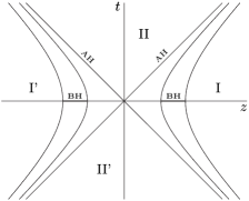
Figure 3: The stationary region ${\cal B}$ of the SC-metric transformed to the coordinates adapted to the boost and rotation symmetries corresponds to the region I under the roof, $z^{2}-t^{2}>0$, where the roof is the acceleration horizon, denoted by AH. Under the roof, there is also another identical stationary region I’ that corresponds to a second black hole accelerated along the symmetry axis in the opposite direction. The non-stationary, radiative regions II, II’ appear above the roof, $z^{2}-t^{2}<0$. This figure covers only the outer part of the spacetime of a uniformly accelerated Kerr black hole outside the exterior black hole horizon (BH). A similar picture, connected with ${\cal D}\cup{\cal D}^{\prime}$, would describe the inner part of the spacetime of a uniformly accelerated Kerr black hole inside the interior black hole horizon.

The axis regularity conditionbivoj ; av-brs

$$\omega(0,z^{2}-t^{2})=0\ ,\mbox{\quad}\lambda(0,z^{2}-t^{2})+\mu(0,z^{2}-t^{2})=0\$$

is satisfied on the outer parts of the axis thanks to Eqs. (23) and (25).

The metric functions (29) are in fact very complicated since we have to use Eqs. (14), (17)–(19), and (27) in order to express them in coordinates $\{t$, $\rho$, $z$, $\varphi\}$. As the Weyl-Papapetrou metric is stationary, via the transformation (27), we get the metric functions in the stationary region bellow the roof. However, using the same expressions for the metric functions $\mu$, $\lambda$, and $\omega$ above the roof, we obtain an analytical continuation of the metric (28) across the roof. It turns out that one has to change the sign of $\epsilon_{3}$ in order to find an analytical continuation of the metric across the null cone of the origin

$$\rho^{2}+z^{2}-t^{2}=R_{3}=0\ .$$ (31)

The non-stationary region above the roof was not included in the Weyl-Papapetrou form, however, it was contained in the original metric (2) in the $\{\tau$, $x$, $y$, $\phi\}$ coordinates.

The region above the roof inside the null cone of the origin ($F<0$ and $\epsilon_{3}>0$ in (16), i.e., the region $\beta_{2}$ in Fig. 4) can be transformed into the cylindrically symmetric metric (see BicSchPRD for the case with hypersurface orthogonal Killing vectors)

$${\rm d}s^{2}={\rm e}^{-2{\tilde{U}}}[{\rm e}^{2{\tilde{\nu}}}(-{\rm d}{\tilde{t}}^{2}+{\rm d}{\tilde{\rho}}^{2})+{\tilde{\rho}}^{2}{\rm d}{\tilde{\varphi}}^{2}]+{\rm e}^{2{\tilde{U}}}({\rm d}{\tilde{z}}+{\tilde{\omega}}{\rm d}{\tilde{\varphi}})^{2}\ ,$$ (32)

where ${\tilde{U}}$, ${\tilde{\nu}}$, and ${\tilde{\omega}}$ are functions of ${\tilde{\rho}}$ and ${\tilde{t}}$, by the transformation

$${\tilde{\rho}}^{2} = {{\cal K}}^{2}\frac{-FG}{A^{4}(x+y)^{4}}\ ,$$

$$\tilde{t} = {{\cal K}}\frac{1+mAxy(x-y)+xy-a^{2}A^{2}x^{2}y^{2}}{A^{2}(x+y)^{2}}\ ,$$

$$\tau = \kappa_{1}{\tilde{z}}+\kappa_{2}{\tilde{\varphi}}\ ,$$

$$\phi = \kappa_{3}{\tilde{z}}+\kappa_{4}{\tilde{\varphi}}\ ,$$

$${\cal K} = \kappa_{2}\kappa_{3}-\kappa_{1}\kappa_{4}\ .$$

Then it can be transformed into the boost-rotation symmetric metric (28) by

$${\tilde{\rho}}^{2} = A^{2}\rho^{2}(t^{2}-z^{2})\ ,$$

$${\tilde{\varphi}} = \varphi\ ,$$

$${\tilde{t}}-{\bar{z}}_{3} = {{\scriptstyle{\frac{1}{2}}}}A(\rho^{2}+t^{2}-z^{2})\ ,$$

$${\tilde{z}} = \frac{1}{A}{\rm arctanh}\left(\frac{t}{z}\right)\ .$$

Similarly by the transformation

$${\hat{t}}^{2} = {\cal K}^{2}\frac{-FG}{A^{4}(x+y)^{4}}\ ,$$

$$\hat{\rho} = {\cal K}\frac{1+mAxy(x-y)+xy-a^{2}A^{2}x^{2}y^{2}}{A^{2}(x+y)^{2}}\ ,$$

$$\tau = \kappa_{1}{\hat{z}}+\kappa_{2}{\hat{\varphi}}\ ,$$

$$\phi = \kappa_{3}{\hat{z}}+\kappa_{4}{\hat{\varphi}}\ ,$$

$${\cal K} = \kappa_{2}\kappa_{3}-\kappa_{1}\kappa_{4}\ ,$$

the region above the roof outside the null cone of the origin ($F<0$ and $\epsilon_{3}<0$ in (16), i.e., the region $\beta_{1}$ in Fig. 4) can be transformed into another cylindrically symmetric metric

$${\rm d}s^{2}={\rm e}^{-2{\hat{U}}}[{\rm e}^{2{\hat{\nu}}}(-{\rm d}{\hat{t}}^{2}+{\rm d}{\hat{\rho}}^{2})+{\hat{t}}^{2}{\rm d}{\hat{\varphi}}^{2}]+{\rm e}^{2{\hat{U}}}({\rm d}{\hat{z}}+{\hat{\omega}}{\rm d}{\hat{\varphi}})^{2}\ ,$$ (33)

where the metric functions ${\hat{U}}$, ${\hat{\nu}}$, and ${\hat{\omega}}$ depend on ${\hat{\rho}}$ and ${\hat{t}}$. Again, it can be transformed into the form (28) by

$${\hat{t}}^{2} = A^{2}\rho^{2}(t^{2}-z^{2})\ ,$$

$${\hat{\varphi}} = \varphi\ ,$$

$${\hat{\rho}}-{\bar{z}}_{3} = {{\scriptstyle{\frac{1}{2}}}}A(\rho^{2}+t^{2}-z^{2})\ ,$$

$${\hat{z}} = \frac{1}{A}{\rm arctanh}\left(\frac{t}{z}\right)\ .$$

Using inverse transformations from the coordinates $\{t$, $\rho$, $z$, $\varphi\}$ into $\{\tau$, $x$, $y$, $\phi\}$, we can find localization of $I^{0}$, $I^{+}$, and ${\cal J}^{+}$ as given in Fig. 4.

One can also determine the ${\cal J}^{+}$ location similarly as was done in haw for the non-spinning C-metric. The SC-metric can be compactified by the conformal factor $\Omega=A(x+y)$. The future null infinity ${\cal J}^{+}$ is then at $\Omega=0$, i.e., $x+y=0$, with the induced metric

$${{\rm d}}{\tilde{s}}_{\cal J}^{2}=G(x)({\rm d}\tau^{2}+{\rm d}\phi^{2})\$$

and the normal vector to ${\cal J}^{+}$

$${\bar{n}}={\tilde{\nabla}}^{\alpha}\Omega\ \partial_{x^{\alpha}}=\frac{AG(x)}{1+(aAx^{2})^{2}}(\partial_{x}-\partial_{y})\ .$$

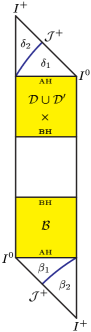
Figure 4: This figure represents the fourth column of Fig. 1, where points $y=\pm\infty$ are identified. The diagram is cut along the line $x+y=0$ where ${\cal J}^{+}$, $I^{+}$, and $I^{0}$ are located. The stationary ${\cal B}$ and non-stationary $\beta_{1}\cup\beta_{2}$ regions correspond to the regions I and II in Fig. 3, respectively. The curves in both triangles represent the null cones of the origin (31) that divide them into the regions $\beta_{1}$ and $\delta_{1}$ outside the null cone and $\beta_{2}$ and $\delta_{2}$ inside the null cone. The stationary region ${\cal D}\cup{\cal D}^{\prime}$ with the curvature singularity denoted by a cross and the triangle above it represent the inner part of the spacetime of a uniformly accelerated Kerr black hole, i.e., a uniformly accelerated white hole with a ring singularity.

V Geodesics in the spinning C-metric

In this section, geodesics in the stationary region $\cal B$ of the SC-metric, especially their stability, are examined. As far as we know, the stability of circular orbits in stationary axisymmetric spacetimes was only studied in the case with an equatorial plane of symmetrybardeen ; olda . The SC-metric (and also other exact solutions, e.g., a superposition of two Schwarzschild or Kerr black holes with different parameters) does not have an equatorial plane of symmetry (see Fig. 2 a). In the following, basic theorems on the stability of solutions of ordinary non-linear differential equationsWalter are employed.

Let us investigate the stability of geodesics in a general stationary spacetime with two Killing vectors, $\partial/\partial t$ and $\partial/\partial\phi$. Later we will apply the results obtained here to the SC-metric (2). We assume the metric in coordinates $\{x^{0},\ x^{1},\ x^{2},\ x^{3}\}$$=\{t,\ X,\ Y,\ \phi\}$ to be of the form

$${\rm d}s^{2}=g_{XX}{\rm d}X^{2}+g_{YY}{\rm d}Y^{2}+g_{tt}{\rm d}t^{2}+2g_{t\phi}{\rm d}t{\rm d}\phi+g_{\phi\phi}{\rm d}\phi^{2}\ ,$$ (34)

where all metric functions depend only on $X$ and $Y$ and $g_{XX}$ and $g_{YY}$ are positive. Let us define ${\cal T}\equiv-g_{tt}$, ${\cal F}\equiv g_{\phi\phi}$, and ${\cal W}\equiv g_{t\phi}$.

Since the metric (34) has two Killing vectors, each freely falling particle carries two conserved quantities

$$U_{\phi} = L=g_{\phi\phi}U^{\phi}+g_{t\phi}U^{t}={\cal F}U^{\phi}+{\cal W}U^{t}\ ,$$

$$U_{t} = -E=g_{t\phi}U^{\phi}+g_{tt}U^{t}={\cal W}U^{\phi}-{\cal T}U^{t}\ ,$$

which imply

$$\dot{\phi} \equiv \frac{{\rm d}\phi}{{\rm d}\tau}=U^{\phi}=\frac{L{\cal T}-E{\cal W}}{{\cal F}{\cal T}+{\cal W}^{2}}\ ,$$

$$\dot{t} \equiv \frac{{\rm d}t}{{\rm d}\tau}=U^{t}=\frac{L{\cal W}+E{\cal F}}{{\cal F}{\cal T}+{\cal W}^{2}}\ .$$ (35)

The norm of the four-velocity $U^{\alpha}=\dot{x}^{\alpha}$ then reads

$$-1=g_{\alpha\beta}U^{\alpha}U^{\beta}=g_{XX}\dot{X}^{2}+g_{YY}\dot{Y}^{2}-{\cal R}-1\$$ (36)

with

$${\cal R}\equiv-1-\frac{1}{{\cal F}{\cal T}+{\cal W}^{2}}(L^{2}{\cal T}-E^{2}{\cal F}-2EL{\cal W})\ .$$ (37)

Thanks to (35), two geodesic equations are satisfied identically while the other two read

$$\ddot{X}+{\cal F}_{1}=0\ ,\mbox{\quad}\ddot{Y}+{\cal F}_{2}=0\ ,$$ (38)

where

$${\cal F}_{1} = {{\scriptstyle{\frac{1}{2}}}}g^{XX}(\ \ g_{XX},_{X}\dot{X}^{2}+2g_{XX},_{Y}\dot{X}\dot{Y}-g_{YY},_{X}\dot{Y}^{2}-{\cal R},_{X})\ ,$$ (39)

$${\cal F}_{2} = {{\scriptstyle{\frac{1}{2}}}}g^{YY}(-g_{XX},_{Y}\dot{X}^{2}+2g_{YY},_{X}\dot{X}\dot{Y}+g_{YY},_{Y}\dot{Y}^{2}-{\cal R},_{Y})\ .$$ (40)

The system of two second-order differential equations (38) can be converted to four first-order differential equations

$$\dot{z}^{\alpha}={\cal F}^{\alpha}\ (z^{\beta})\ ,\mbox{\quad}{\cal F}^{\alpha}=(z^{2},\ -{\cal F}_{1},\ z^{4},\ -{\cal F}_{2})$$ (41)

introducing new variables $z^{\alpha}$

$$z^{1}\equiv X\ ,\mbox{\quad}z^{2}\equiv\dot{X}\ ,\mbox{\quad}z^{3}\equiv Y\ ,\mbox{\quad}z^{4}\equiv\dot{Y}\ .$$ (42)

Stationary (equilibrium) points of the system (41), $z^{\alpha}_{0}$, are given by ${\cal F}^{\alpha}(z^{\beta}_{0})=0$, i.e.,

$$z^{2} = \dot{X}=0\ ,\mbox{\quad}z^{4}=\dot{Y}=0\ ,\mbox{\quad}\mbox{i.e.,}\mbox{\quad}{\cal R}(z_{0}^{\alpha})=0\ ,$$ (43)

$${\cal F}_{1} = -{{\scriptstyle{\frac{1}{2}}}}g^{XX}{\cal R},_{X}(z_{0}^{\alpha})=0\ ,$$ (44)

$${\cal F}_{2} = -{{\scriptstyle{\frac{1}{2}}}}g^{YY}{\cal R},_{Y}(z_{0}^{\alpha})=0\ .$$ (45)

One can eliminate $E$ and $L$ from Eqs. (44), (45) and derive the equation for the stationary points $X_{0}$, $Y_{0}$

$$({\cal F},_{[X}{\cal T},_{Y]})^{2}-4({\cal T},_{[X}{\cal W},_{Y]})({\cal F},_{[X}{\cal W},_{Y]})=0\$$ (46)

and, using also Eq. (43), express $E$ and $L$ in terms of $X_{0}$ and $Y_{0}$.

Since the system (41) is autonomous, its linearization may help to determine the stability of its stationary pointsWalter . The linearized form of (41) in the neighbourhood of a stationary point $z_{0}^{\alpha}$ is

$$\dot{z}^{\alpha}=A^{\alpha}_{\beta}(z^{\beta}-z_{0}^{\beta})\ ,$$

where

$$A^{\alpha}_{\beta}\equiv\frac{\partial{\cal F}^{\alpha}}{\partial{z^{\beta}}}(z_{0}^{\gamma})=\pmatrix{0&1&0&0\cr-{\cal F}^{(0)}_{1},_{X}&0&-{\cal F}^{(0)}_{1},_{Y}&0\cr 0&0&0&1\cr-{\cal F}^{(0)}_{2},_{X}&0&-{\cal F}^{(0)}_{2},_{Y}&0}$$

is a constant matrix with eigenvalues

$$\lambda_{\alpha}=\pm\sqrt{{{\scriptstyle{\frac{1}{2}}}}}\sqrt{-{\cal F}^{(0)}_{1},_{X}-{\cal F}^{(0)}_{2},_{Y}\pm\sqrt{({\cal F}^{(0)}_{1},_{X}-{\cal F}^{(0)}_{2},_{Y})^{2}+4{\cal F}^{(0)}_{1},_{Y}{\cal F}^{(0)}_{2},_{X}}}\ ,$$ (47)

with ${\cal F}^{(0)}_{1},_{X}\equiv{\cal F}_{1},_{X}(z_{0}^{\gamma})$, etc. If all Re$\lambda_{\alpha}$ were negative the equilibrium point of (41) would be asymptotically stable and if at least one Re$\lambda_{\alpha}$ were positive the equilibrium point of (41) would be unstable. If max$\{$Re$\lambda_{\alpha}\}$ were zero the studied point could be stable, however, further examinations would be necessary. Since $\lambda_{1}+\lambda_{2}=\lambda_{3}+\lambda_{4}=0$, the stationary point $z_{0}^{\alpha}$ is unstable if Re$\lambda_{\alpha}\not=0$ for any $\alpha$ and could be stable only if Re$\lambda_{\alpha}=0$ for all $\alpha$, i.e., for

$${\cal F}^{(0)}_{1},_{X}{\cal F}^{(0)}_{2},_{Y}>{\cal F}^{(0)}_{1},_{Y}{\cal F}^{(0)}_{2},_{X}\ ,\mbox{\quad}\mbox{i.e.,}\mbox{\quad}{\cal R}^{(0)},_{XX}{\cal R}^{(0)},_{YY}>{\cal R}^{(0)},_{XY}\ ^{2}\ ,$$

$${\cal F}^{(0)}_{1},_{X}>0\ ,\mbox{\quad}{\cal F}^{(0)}_{2},_{Y}>0\ ,\mbox{\quad}\mbox{\quad}\mbox{\quad}\ \mbox{i.e.,}\mbox{\quad}{\cal R}^{(0)},_{XX}<0\ ,\mbox{\quad}{\cal R}^{(0)},_{YY}<0\ ,$$ (48)

i.e., if the function ${\cal R}$ has a local maximum in the equilibrium point or if

$${\cal F}^{(0)}_{1},_{X}={\cal F}^{(0)}_{2},_{Y}={\cal F}^{(0)}_{1},_{Y}{\cal F}^{(0)}_{2},_{X}=0\ ,\mbox{\quad}$$

i.e., $${\cal R}^{(0)},_{XX}={\cal R}^{(0)},_{YY}={\cal R}^{(0)},_{XY}=0\ .$$ (49)

In order to determine whether the stationary points given by (46) and satisfying (48) or (49) are indeed stable, we employ the Lyapunov method. The Lyapunov function for (41) is a function $V$ of four independent variables $z^{\alpha}$ satisfying in an open neighbourhood of an equilibrium point $z_{0}^{\alpha}$ the conditions

$$V(z^{\alpha})>0\mbox{\quad}\mbox{for}\mbox{\quad}z^{\alpha}\not=z_{0}^{\alpha}\ ,\mbox{\quad}V(z_{0}^{\alpha})=0\ ,$$ (50)

$$V^{\prime}\equiv V,_{z^{\alpha}}{\cal F}^{\alpha}\leq 0\ .$$ (51)

Notice that $V^{\prime}$ is the directional derivative of $V$ in the direction of ${\cal F}^{\alpha}$, $V^{\prime}=\lim_{t\rightarrow 0}[V(z^{\alpha}+t{\cal F}^{\alpha})-V(z^{\alpha})]/t$. If such a function exists then the equilibrium point $z_{0}^{\alpha}$ is stable, however, there is not a general method how to find it.

It can be shown that

$$V=g_{XX}{z_{2}}^{2}+g_{YY}{z_{4}}^{2}-{\cal R}\ ,$$ (52)

which satisfies $V^{\prime}=0$ identically, is the Lyapunov function for the system (41) if ${\cal R}$ is negative in the neighbourhood of the equilibrium point $z_{0}^{\alpha}$, i.e., if ${\cal R}$ has a local maximum in $z_{0}^{\alpha}$ since ${\cal R}(z_{0}^{\alpha})=0$. Thus, equilibrium points satisfying (48) are indeed stable.

In the special case ${\cal W}=0$ with hypersurface orthogonal Killing vectors, ${\cal R}\sim(E^{2}-V_{\mbox{ef}}^{2})/E^{2}$, where $V_{\mbox{ef}}$ is the effective potential. A local maximum of ${\cal R}$ then corresponds to a local minimum of $V_{\mbox{ef}}$.

To summarize: The stationary points $X=X_{0}$ and $Y=Y_{0}$ given by (46) are stable if ${\cal R}$ (37) has a local maximum there.

Let us apply the foregoing general considerations to the SC-metric (2). The corresponding computations are rather complicated and thus we present only the main results here.

The condition (46) for stationary points is a polynomial of the order 12 in $x$ and $y$ and for $a=0$ it reduces to Eq. (10) in av-geod . The stationary points $x_{0}$, $y_{0}$ in the ${\cal B}$ region are plotted in Fig. 5. As in the non-spinning caseav-geod , the stationary points $x_{0}=0$ correspond to null geodesics, stationary points with $x_{0}>0$ and $x_{0}<0$ to timelike and spacelike geodesics, respectively.

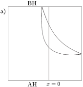
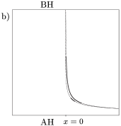
Figure 5: Stationary points in the ${\cal B}$ region of the SC-metric for a) $m=1$, $a=1/2$, $A=1/10$; b) $m=1/5$, $a=1/6$, $A=1/100$ – stable equilibrium points are highlighted, the upper and lower curves correspond to retrograde and prograde orbits, respectively.

In contrast to the non-spinning case, there now appear two curves in Fig. 5 – the upper and the lower one corresponding to retrograde ($L<0$) and prograde ($L>0$) orbits, respectively.

Using Eq. (48), one can show that for $A$ small, there exist both retrograde and prograde stable orbits (Fig. 5 b). As was shown in av-geod , these geodesics correspond to co-accelerated test particles orbiting the uniformly accelerated black hole. If the parameters $E$ and $L$ are perturbed sufficiently the test particle falls under the black hole or acceleration horizon.

VI Conclusion

If conditions (4) are satisfied there are four stationary regions in the SC-metric. Each of them can be transformed into a different Weyl-Papapetrou metric by (8)–(12). The most physically important region ${\cal B}$ in the Weyl-Papapetrou coordinates represents the gravitational field of a “spinning rod” (the black hole horizon) and a semi-infinite line mass that are held in equilibrium by a spinning string. There is an ergoregion in the vicinity of the black hole horizon and a region with closed timelike curves in the neighbourhood of the spinning string (see Fig. 2 a). In the limit the acceleration $A$ $\rightarrow 0$, there remains just the “spinning rod”, which corresponds to the “exterior” of the Kerr metric. Through a further transformation to the coordinates adapted to the boost and rotation symmetries new non-stationary radiative regions appear. It turns out that these regions are already contained in the original form (2) of the SC-metric (see Fig. 4).

Another stationary region ${\cal D}\cup{\cal D}^{\prime}$ corresponds to a uniformly accelerated superposition of a spinning white hole and a ring singularity, which represents a uniformly accelerated “interior” of the Kerr solution, i.e., the region bellow the inner horizon up to $r\rightarrow-\infty$. A timelike curve in the Kerr metric can start in the external, asymptotically flat region, cross two horizons, pass through the ring singularity, and emerge in another asymptotically flat white hole region, where gravity is repulsive. Similarly, in the SC-metric, a timelike curve starting in the region ${\cal B}$ can cross two horizons and debouch in the region ${\cal D}\cup{\cal D}^{\prime}$. Then, if it is not co-accelerated it crosses the null cone of the origin and reaches $I^{+}$ (see Fig. 4).

In Sec. V, the stability of geodesics corresponding to equilibrium points in a general stationary spacetime with two symmetries was studied. Using the Lyapunov method it can be shown that an equilibrium point is stable if the function ${\cal R}$ of two variables (37) has a local maximum there. It turns out that for the SC-metric there exist stable prograde and retrograde orbits corresponding to co-accelerated particles orbiting the uniformly accelerated spinning black hole.

References

(1)
T. Levi-Civita, d einsteiniani in campi newtoniani,
Rend. Acc. Lincei
27, 343 (1918).
(2)
H. Weyl, Bemerkung über die axisymmetrischen lösungen der
Einsteinschen Gravitationsgleinchungen, Ann. d. Phys 59, 185 (1919).
(3)
W. Kinnersley and M. Walker, Uniformly Accelerating
Charged Mass in General Relativity,
Phys. Rev. D 2, 1359 (1970).
(4)
W. B. Bonnor, The sources of the vacuum C-metric,
Gen. Rel. Grav. 15, 535 (1983).
(5)
J. Bičák and B. G. Schmidt, Asymptotically flat radiative
space-times with boost-rotation
symmetry: The general structure, Phys. Rev. D 40, 1827 (1989).
(6)
J. Bičák, Selected solutions of Einstein’s field equations:
their role in general relativity
and astrophysics, in Einstein’s Field Equations and Their
Physical Meaning (Ed. B. G. Schmidt),
Springer Verlag, Berlin – New York (2000).
(7)
V. Pravda and A. Pravdová, Boost-rotation symmetric spacetimes –
review,
Czech. J. Phys. 50, 333 (2000); see also gr-qc/0003067.
(8)
F. H. J. Cornish and W. J. Uttley, The interpretation of the C metric. The charged case when
, Gen. Rel. Grav. 27, 735 (1995).
(9)
F. J. Ernst, Generalized C-metric, J. Math. Phys. 19, 1986 (1978).
(10)
H. F. Dowker and S. N. Thambyahpillai, Many Accelerating Black Holes,
gr-qc/0105044 (2001).
(11)
J. F. Plebański and M. Demiański,
Rotating, charged and uniformly accelerating
mass in general relativity, Ann. Phys. (USA) 98, 98 (1976).
(12)
H. Farhoosh and R. L. Zimmerman, Surfaces of infinite
red-shift around a uniformly accelerating
and rotating particle, Phys. Rev. D 21, 2064 (1980).
(13)
J. Bičák and V. Pravda, Spinning C metric: Radiative spacetime with accelerating,
rotating black holes, Phys. Rev. D 60, 044004 (1999).
(14)
P. S. Letelier and S. R. Oliveira, Uniformly accelerated black holes,
Phys. Rev. D 64, 064005 (2001).
(15)
A. Pravdová and V. Pravda, Boost-rotation symmetric
vacuum spacetimes with spinning sources, to appear in J. Math. Phys.;
see also gr-qc/0107068 (2001).
(16)
I. Ciufolini, Gravitomagnetism and status of the LAGEOS III experiment,
Class. Quantum Grav. 11, A73 (1994).
(17)
B. B. Godfrey, Horizons in Weyl metrics exhibiting extra symmetries,
Gen. Rel. Grav. 3, 3 (1972).
(18)
P. S. Letelier, Static and stationary multiple soliton solutions to the Einstein
equations, J. Math. Phys. 26, 467 (1985).
(19)
P. S. Letelier and S. R. Oliveira, Double Kerr-NUT spacetimes:
spinning strings and spinning rods, Phys. Lett. A 238, 101 (1998).
(20)
W. B. Bonnor, The interactions between two classical spinning particles,
Class. Quantum Grav. 18, 1382
(2001).
(21)
F. H. J. Cornish and W. J. Uttley, The Interpretation of the C Metric.
The Vacuum Case, Gen. Rel. Grav. 27, 439 (1995).
(22)
D. Kramer, H. Stephani, E. Herlt, and M. A. H. MacCallum,
Exact solutions of Einstein’s field equations (Ed. E. Schmutzer),
Cambridge Univ. Press, Cambridge (1980).
(23)
W. B. Bonnor and N. S. Swaminarayan, An Exact Solution for
Uniformly Accelerated Particles in General Relativity,
Z. Phys. 177, 240 (1964).
(24)
S. W. Hawking and S. F. Ross, Loss of quantum coherence
through scattering off virtual black holes, Phys. Rev. D 56,
6403 (1997).
(25)
J. M. Bardeen, Stability of circular orbits in stationary, axisymmetric spacetimes,
ApJ 161, 103 (1970).
(26)
O. Semerák, M. Žáček, and T. Zellerin, Test-particle motion in
superposed Weyl field, Mon. Not. R. Astron. Soc. 308, 705 (1999).
(27)
W. Walter, Ordinary Differential Equations,
Springer-Verlag, New York (1998).
(28)
V. Pravda and A. Pravdová, Co-accelerated particles
in the C-metric, Class. Quantum Grav. 18, 1205
(2001).