Post-Newtonian gravitational radiation and equations of motion via direct integration of the relaxed Einstein equations.
II. Two-body equations of motion to second post-Newtonian order, and radiation-reaction to 3.5 post-Newtonian order

Abstract

We derive the equations of motion for binary systems of compact bodies in the post-Newtonian (PN) approximation to general relativity. Results are given through 2PN order (order $(v/c)^{4}$ beyond Newtonian theory), and for gravitational radiation reaction effects at 2.5PN and 3.5PN orders. The method is based on a framework for direct integration of the relaxed Einstein equations (DIRE) developed earlier, in which the equations of motion through 3.5PN order can be expressed in terms of Poisson-like potentials that are generalizations of the instantaneous Newtonian gravitational potential, and in terms of multipole moments of the system and their time derivatives. All potentials are well defined and free of divergences associated with integrating quantities over all space. Using a model of the bodies as spherical, non-rotating fluid balls whose characteristic size $s$ is small compared to the bodies’ separation $r$, we develop a method for carefully extracting only terms that are independent of the parameter $s$, thereby ignoring tidal interactions, spin effects, and internal self-gravity effects. Through 2.5PN order, the resulting equations agree completely with those obtained by other methods; the new 3.5PN back-reaction results are shown to be consistent with the loss of energy and angular momentum via radiation to infinity.

I Introduction and Summary

This is the second in a series of papers which will treat motion and gravitational radiation in the post-Newtonian approximation to general relativity. While this is a problem that dates back to the beginnings of general relativity, it has recently taken on added observational importance because of the need for extremely accurate theoretical gravitational waveform templates for analysis of data taken by laser interferometric gravitational-wave detectors [1]. Specifically, for waves from inspiralling binary systems of compact objects (neutron stars or black holes), equations of motion and gravitational waveforms accurate to at least third post-Newtonian order (order $(v/c)^{6}$) beyond the initial Newtonian or quadrupole approximation are needed.

In paper I [2], we laid out the foundations of our method of Direct Integration of the Relaxed Einstein Equations (DIRE). We rewrote the Einstein equations as a flat spacetime wave equation together with a harmonic gauge condition (the “relaxed” Einstein equations), and solved them formally in terms of a retarded integral over the past null cone of the field point. Because the “source” contains both the material stress-energy tensor and the stress-energy contributions of the gravitational fields themselves, it was necessary to iterate the integrals repeatedly to obtain successively higher-order approximations to a solution in powers of $\epsilon\sim(v/c)^{2}\sim(Gm/rc^{2})$. Each power of $\epsilon$ represents one “post-Newtonian” (PN) order in the series ($\epsilon^{1/2}$ represents one half, or 0.5PN orders). Despite the fact that the field contributions to the integrals extend over all spacetime, we demonstrated that no infinite or ill-defined integrals occurred, even in slow-motion, multipole expansions, and found a simple prescription for evaluating the finite contributions of all integrals. This was true for calculations of the metric both in the near zone and in the far zone.

To complete the solution of Einstein’s equations, one needs equations of motion for the system. For this, one needs the spacetime metric evaluated for field points within the near zone, corresponding to a sphere of radius $\cal R\sim$ one gravitational wavelength. In Paper I, we expressed this near-zone metric explicitly through order $\epsilon^{7/2}$ beyond the Newtonian approximation, corresponding to 3.5 post-Newtonian (PN) order, in terms of instantaneous, Poisson-like integrals and their generalizations, of the form, for example,

$$P(f)\equiv{1\over{4\pi}}\int_{\cal M}{{f(t,{\bf x}^{\prime})}\over{|{\bf x}-{\bf x}^{\prime}|}}d^{3}x^{\prime}\,,$$ (1)

where the integration is confined to the near zone $\cal M$, and only that part of the integral that is independent of $\cal R$ is kept.

It is the purpose of this paper to evaluate these integrals explicitly for a binary system of non-spinning, spherically symmetric bodies whose size is much smaller than their separation. We will carry this evaluation through 2PN order, and will also evaluate the leading radiation-reaction contributions at 2.5PN order, together with the first post-Newtonian corrections to radiation reaction, at 3.5PN order. The extremely lengthy derivation of the non-radiative 3PN contributions will be reserved for future publications. The resulting equations have the form

$${{d^{2}{\bf x}}\over{dt^{2}}} = -{m\over r^{2}}{\bf n}+{m\over r^{2}}\bigl{[}\,{\bf n}(A_{PN}+A_{2PN}+A_{3PN})+{\dot{r}}{\bf v}(B_{PN}+B_{2PN}+B_{3PN})\bigr{]}$$ (3)

$$+{8\over 5}\eta{m\over r^{2}}{m\over r}\bigl{[}\dot{r}{\bf n}(A_{2.5PN}+A_{3.5PN})-{\bf v}(B_{2.5PN}+B_{3.5PN})\bigr{]}\,,$$

where ${\bf x}\equiv{\bf x}_{1}-{\bf x}_{2}$, $r\equiv|{\bf x}|$, ${\bf n}\equiv{\bf x}/r$, $m\equiv m_{1}+m_{2}$, $\eta\equiv m_{1}m_{2}/m^{2}$, ${\bf v}\equiv{\bf v}_{1}-{\bf v}_{2}$, and $\dot{r}=dr/dt$. We use units in which $G=c=1$. The leading term is Newtonian gravity. The other terms on the first line are the “conservative” or non-dissipative terms, of even PN order, while those on the second line are dissipative radiation-reaction terms, of odd-half PN order. The coefficients $A$ and $B$ are given explicitly by

$$A_{PN} = -(1+3\eta)v^{2}+{3\over 2}\eta{\dot{r}}^{2}+2(2+\eta)m/r\,,$$ (5)

$$B_{PN} = 2(2-\eta)\,,$$ (6)

$$A_{2PN} = -\eta(3-4\eta)v^{4}+{1\over 2}\eta(13-4\eta)v^{2}m/r+{3\over 2}\eta(3-4\eta)v^{2}{\dot{r}}^{2}$$ (8)

$$+(2+25\eta+2\eta^{2}){\dot{r}}^{2}m/r-{15\over 8}\eta(1-3\eta){\dot{r}}^{4}-{3\over 4}(12+29\eta)(m/r)^{2}\,,$$

$$B_{2PN} = {1\over 2}\eta(15+4\eta)v^{2}-{3\over 2}\eta(3+2\eta){\dot{r}}^{2}-{1\over 2}(4+41\eta+8\eta^{2})m/r\,,$$ (9)

$$A_{2.5PN} = 3v^{2}+{17\over 3}m/r\,,$$ (10)

$$B_{2.5PN} = v^{2}+3m/r\,,$$ (11)

$$A_{3.5PN} = -{3\over 28}(61+70\eta)v^{4}-{1\over 42}(519-1267\eta)v^{2}m/r+{15\over 4}(19+2\eta)v^{2}\dot{r}^{2}$$ (13)

$$-{1\over 4}(147+188\eta)\dot{r}^{2}m/r-70\dot{r}^{4}-{23\over 14}(43+14\eta)(m/r)^{2}\,,$$

$$B_{3.5PN} = -{1\over 28}(313+42\eta)v^{4}+{1\over 42}(205+777\eta)v^{2}m/r+{3\over 4}(113+2\eta)v^{2}\dot{r}^{2}$$ (15)

$$-{1\over 12}(205+424\eta)\dot{r}^{2}m/r-75\dot{r}^{4}-{1\over 42}(1325+546\eta)(m/r)^{2}\,.$$

The 1PN coefficients are standard; the 2PN and 2.5PN terms agree completely with results derived by Damour and Deruelle [3, 4], Kopeiken and Grishchuk [5, 6], Blanchet et al. [7], and Itoh et al. [8]. However, the 2.5PN terms differ from those derived, for example from a Burke-Thorne type radiation-reaction potential given by $\Phi_{RR}=-(1/5)x^{i}x^{j}d^{5}{\cal I}^{<ij>}/dt^{5}$, where ${\cal I}^{<ij>}$ is the system’s trace-free quadrupole moment (see, e.g. §36.11 of [9]). Iyer and Will [10, 11] showed that there is a two-parameter “gauge” freedom in the radiation reaction equations at 2.5PN order (and a six-parameter freedom at 3.5 PN order), within which the different equations of motion yield identical results for the net energy and angular momentum radiated. The 2.5PN terms shown are thus observationally equivalent to the Burke-Thorne radiation reaction equations. The 3.5PN terms are new; it can be shown that they correspond to a specific choice of the six Iyer-Will gauge parameters, and thus automatically generate the proper post-Newtonian corrections to energy and angular momentum loss. Schäfer and Jaranowski [12, 13, 14] also derived 2PN, 2.5PN and 3.5PN contributions to the equations of motion in a Hamiltonian formulation. The 3PN contributions to the equations of motion have also been reported by several groups [15, 16, 17, 18, 19].

The remainder of this paper is devoted to the details supporting these results. In Sec. II we review the basic equations needed to find equations of motion to the order needed. Section III specializes to binary systems of spherical “pointlike” bodies, and derives the equations of motion for each body correct to 2PN order. Section IV repeats the process for the 2.5PN and 3.5PN terms. In Sec. V we transform to an effective one-body relative equation of motion. Concluding remarks are made in Sec. VI. Detailed points are reserved for a series of Appendices.

Our conventions and notation generally follow those of [9, 20]. Greek indices run over four spacetime values 0, 1, 2, 3, while Latin indices run over three spatial values 1, 2, 3; commas denote partial derivatives with respect to a chosen coordinate system, while semicolons denote covariant derivatives; repeated indices are summed over; $\eta^{\mu\nu}=\eta_{\mu\nu}={\rm diag}(-1,1,1,1)$; $g\equiv\det(g_{\mu\nu})$; $a^{(ij)}\equiv(a^{ij}+a^{ji})/2$; $a^{[ij]}\equiv(a^{ij}-a^{ji})/2$; $\epsilon^{ijk}$ is the totally antisymmetric Levi-Civita symbol $(\epsilon^{123}=+1)$. We use a multi-index notation for products of vector components and partial derivatives, and for multiple spatial indices: $x^{ij\dots k}\equiv x^{i}x^{j}\dots x^{k}$, $\nabla^{ij\dots k}\equiv\nabla^{i}\nabla^{j}\dots\nabla^{k}$, with a capital letter superscript denoting an abstract product of that dimensionality: $x^{Q}\equiv x^{i_{1}}x^{i_{2}}...x^{i_{q}}$ and $\nabla^{Q}\equiv\nabla^{i_{1}}\nabla^{i_{2}}...\nabla^{i_{q}}$. Also, for a tensor of rank $Q$, $f^{Q}\equiv f^{i_{1}i_{2}\dots i_{q}}$. The notation $f^{Q}g^{Q}$ denotes a complete contraction over the $q$ indices. Spatial indices are freely raised and lowered with $\delta^{ij}$ and $\delta_{ij}$.

II Equations of motion of compact binary systems: basic equations

A Structure of the near-zone metric to 3.5PN order

We begin by reviewing key results from Paper I. We defined the “field” $h^{\alpha\beta}$ by

$$h^{\alpha\beta}\equiv\eta^{\alpha\beta}-(-g)^{1/2}g^{\alpha\beta}\;,$$ (16)

where $g^{\alpha\beta}$ is the space time metric. In deDonder or harmonic coordinates defined by the gauge condition $h^{\alpha\beta},_{\beta}=0$, the Einstein equations take the form

$$\Box h^{\alpha\beta}=-16\pi{\tau}^{\alpha\beta}\;,$$ (17)

where $\Box$ is the flat-spacetime wave operator, and ${\tau}^{\alpha\beta}$ is made up of the material stress-energy tensor $T^{\alpha\beta}$ and the contribution of all the non-linear terms in Einstein’s equations. We defined a notation for specific components of the field $h^{\alpha\beta}$:

$$N \equiv h^{00}\sim O(\epsilon)\,,$$ (18)

$$K^{i} \equiv h^{0i}\sim O(\epsilon^{3/2})\,,$$ (19)

$$B^{ij} \equiv h^{ij}\sim O(\epsilon^{2})\,,$$ (20)

$$B \equiv \sum_{i}h^{ii}\sim O(\epsilon^{2})\,,$$ (21)

where we show the leading-order dependence on $\epsilon$ in the near zone. To the necessary orders for calculating the equations of motion to 3.5PN order, the components of the physical metric are given in terms of $N$, $K^{i}$, $B^{ij}$ and $B$ by

$$g_{00} = -(1-{1\over 2}N+{3\over 8}N^{2}-{5\over 16}N^{3}+{35\over 128}N^{4})+{1\over 2}B(1-{1\over 2}N+{3\over 8}N^{2})$$ (23)

$$+{1\over 4}(B^{ij}B^{ij}-{1\over 2}B^{2})+{1\over 2}K^{j}K^{j}-{3\over 4}NK^{j}K^{j}+O(\epsilon^{5})\,,$$

$$g_{0i} = -K^{i}(1-{1\over 2}N-{1\over 2}B+{3\over 8}N^{2})-K^{j}B^{ij}+O(\epsilon^{9/2})\,,$$ (24)

$$g_{ij} = \delta^{ij}(1+{1\over 2}N-{1\over 8}N^{2}+{1\over 16}N^{3}-{1\over 4}NB+{1\over 2}K^{k}K^{k})$$ (26)

$$+B^{ij}-{1\over 2}B\delta^{ij}-K^{i}K^{j}+{1\over 2}NB^{ij}+O(\epsilon^{4})\,,$$

$$(-g) = 1+N-B-NB+K^{i}K^{i}+O(\epsilon^{4})\,.$$ (27)

The potentials $N$, $K^{i}$, $B^{ij}$ and $B$ must also be expanded to an appropriate order:

$$N = \epsilon(4U_{\sigma}+\epsilon N_{1}+\epsilon^{3/2}N_{1.5}+\epsilon^{2}N_{2}+\epsilon^{5/2}N_{2.5}+\epsilon^{3}N_{3}+\epsilon^{7/2}N_{3.5})+O(\epsilon^{5})\,,$$ (28)

$$K^{i} = \epsilon^{3/2}(4V_{\sigma}^{i}+\epsilon K_{2}^{i}+\epsilon^{3/2}K_{2.5}^{i}+\epsilon^{2}K_{3}^{i}+\epsilon^{5/2}K_{3.5}^{i})+O(\epsilon^{9/2})\,,$$ (29)

$$B = \epsilon^{2}(B_{1}+\epsilon^{1/2}B_{1.5}+\epsilon B_{2}+\epsilon^{3/2}B_{2.5}+\epsilon^{2}B_{3}+\epsilon^{5/2}B_{3.5})+O(\epsilon^{5})\,,$$ (30)

$$B^{ij} = \epsilon^{2}(B_{2}^{ij}+\epsilon^{1/2}B_{2.5}^{ij}+\epsilon B_{3}^{ij}+\epsilon^{3/2}B_{3.5}^{ij})+O(\epsilon^{4})\,,$$ (31)

where the subscript on each term indicates the level (1PN, 2PN, 2.5PN, etc.) of its leading contribution to the equations of motion. Notice that our separate treatment of $B$ and $B^{ij}$ leads to the slightly awkward notational circumstance that, for example, $B_{2}^{ii}=B_{1}$. In Paper I, we obtained explicit near-zone expressions for each of the terms in Eq. (31) in terms of Poisson-like potentials

$$P(f) \equiv {1\over{4\pi}}\int_{\cal M}{{f(t,{\bf x}^{\prime})}\over{|{\bf x}-{\bf x}^{\prime}|}}d^{3}x^{\prime}\,,\quad\nabla^{2}P(f)=-f\,,$$ (32)

$$\Sigma(f) \equiv \int_{\cal M}{{\sigma(t,{\bf x}^{\prime})f(t,{\bf x}^{\prime})}\over{|{\bf x}-{\bf x}^{\prime}|}}d^{3}x^{\prime}=P(4\pi\sigma f)\,,$$ (33)

and various generalizations [for definitions, see Paper I, Eqs. (4.10) – (4.16)], and in terms of source multipole moments, such as ${\cal I}^{ij}\equiv\int_{\cal M}\tau^{00}x^{ij}d^{3}x$ [for definitions, see Paper I, Eqs. (2.14) and (4.5) – (4.7)]. The integrations are over a constant time hypersurface $\cal M$ that extends to a radius ${\cal R}\sim$ one gravitational wavelength from the source. In Paper I, we showed that, even for Poisson potentials where the function $f$ does not have compact support, all contributions to the field $h^{\mu\nu}$ from the integration over $\cal M$ that depend on $\cal R$ cancel corresponding contributions from that part of the field point’s past null cone that is outside $\cal R$, and thus that any $\cal R$-dependent terms that appear in a given integral can simply be discarded.

The potentials given in Paper I were expressed in terms of specific source densities given by

$$\sigma \equiv T^{00}+T^{ii}\,,$$ (34)

$$\sigma^{i} \equiv T^{0i}\,,$$ (35)

$$\sigma^{ij} \equiv T^{ij}\,.$$ (36)

For example, in Eq. (31),

$$U_{\sigma} \equiv \int_{\cal M}{{\sigma(t,{\bf x}^{\prime})}\over{|{\bf x}-{\bf x}^{\prime}|}}d^{3}x^{\prime}=P(4\pi\sigma)=\Sigma(1)\,,$$ (37)

$$V_{\sigma}^{i} \equiv \int_{\cal M}{{\sigma^{i}(t,{\bf x}^{\prime})}\over{|{\bf x}-{\bf x}^{\prime}|}}d^{3}x^{\prime}=P(4\pi\sigma^{i})=\Sigma^{i}(1)\,.$$ (38)

Explicit expressions for the remaining terms in Eq. (31) can be found in Paper I, Eqs. (5.2), (5.4), (5.8), (5.10), (6.2), and (6.4).

B Model of the material sources

We model the material sources in the binary system as perfect fluid, having stress-energy tensor

$$T^{\alpha\beta}\equiv(\rho+p)u^{\alpha}u^{\beta}+pg^{\alpha\beta}\;,$$ (39)

where $\rho$ and $p$ are the locally measured energy density and pressure, respectively, and $u^{\alpha}$ is the four-velocity of an element of fluid. We will assume the bodies to be non-rotating (the effects of spin will be treated in future publications), spherically symmetric in their comoving rest frames, and small compared to their separation, so that tidal distortions can be ignored.

Our goal is to determine all contributions to the equations of motion that are independent of the internal structure, size, and shape of the bodies. We are less interested in formal rigor than in having a robust method that captures all the effects without missing any. One approach to this has been to assume a “delta-function” or distributional form for the stress-energy tensor. This has been criticized because such a source is fundamentally incompatible with general relativity, and because it leads to divergences related to the infinite self-field of a point mass. A number of methods have been developed in order to extract the finite part of such divergent expressions, including the Hadamard partie finie technique (for a recent review, see [21]. Another approach is related to that of Einstein, Infeld and Hoffman (EIH) [22]: expand the vacuum Einstein equations in a post-Newtonian expansion and match the solutions to fields representing the near-zone, Schwarzschild-like field of a static, spherical body. The consistency conditions imposed by the matching lead to constraints on the motion of the bodies that yield the equations of motion. This has been carried out to 2.5PN order by Itoh et al. [23, 8], exploiting a “strong-field point particle” scaling method of Futamase [24].

A third approach is to treat the bodies realistically as fluid balls with internal energy, supported against their self gravity by pressure governed by an equation of state. In this case, the mass of each body is composed of rest mass, internal energy and self-gravitational binding energy, and the center of mass is defined accordingly. However, at Newtonian and 1PN order, when finite-size effects such as tidal interactions are ignored, it turns out that all vestiges of the internal structure are “effaced”, in the language of Damour [4], and the final 1PN equations of motion depend on one and only one mass as defined above. This procedure can be seen in detail, for example, in [25], §6.2, where the calculation is actually carried out in the parametrized post-Newtonian (PPN) framework, which encompasses a class of metric theories of gravity. In many alternative theories, such as scalar-tensor gravity, the effacement is violated, and the equations of motion depend on various masses, such as inertial mass $m$, active gravitational mass $m_{A}$, and passive gravitational mass $m_{P}$, which may differ by amounts depending on the bodies’ gravitational binding energy. In GR, the PPN parameters are such that all three masses are identical.

In fact, the 1PN equations of motion derived from this method are identical to those obtained from a “delta” function method in which one systematically throws away all terms that are singular when evaluated on each body’s world line. At 1PN order, the results are in keeping with the idea that general relativity satisfies the Strong Equivalence Principle (see §3.3 of [25]), part of which implies that the motion of bound bodies is independent of their internal structure, provided that tidal effects can be ignored. Kopeikin [5] extended this to 2PN order, with results consistent with the Strong Equivalence Principle.

Our approach will be intermediate between the “delta-function” model and the full equilibrium fluid ball method. We will neglect pressure $p$ and internal energy density, and treat the bodies as balls of baryons characterized by the “conserved” baryon mass density $\rho^{*}$, given by

$$\rho^{*}\equiv mn\sqrt{-g}u^{0}\,,$$ (40)

where $m$ is the rest mass per baryon, $n$ is the baryon number density, and $g\equiv\det(g_{\mu\nu})$. From the conservation of baryon number, expressed in covariant terms by $(nu^{\alpha})_{;\alpha}=0=(\sqrt{-g}nu^{\alpha})_{,\alpha}$, we see that $\rho^{*}$ obeys the non-covariant, but exact, continuity equation

$$\partial\rho^{*}/\partial t+\nabla\cdot(\rho^{*}{\bf v})=0\,,$$ (41)

where $v^{i}=u^{i}/u^{0}$, and spatial gradients and dot products use a Cartesian metric. In terms of $\rho^{*}$, the stress-energy tensor takes the form

$$T^{\alpha\beta}=\rho^{*}(-g)^{-1/2}u^{0}v^{\alpha}v^{\beta}\,,$$ (42)

where $v^{\alpha}=(1,v^{i})$. We define the baryon rest mass, center of baryonic mass, velocity and acceleration of each body by the formulae

$$m_{A} \equiv \int_{A}\rho^{*}d^{3}x\,,$$ (43)

$${\bf x}_{A} \equiv (1/m_{A})\int_{A}\rho^{*}{\bf x}^{i}d^{3}x\,,$$ (44)

$${\bf v}_{A} \equiv d{\bf x}_{A}/dt=(1/m_{A})\int_{A}\rho^{*}{\bf v}^{i}d^{3}x\,,$$ (45)

$${\bf a}_{A} \equiv d{\bf v}_{A}/dt=(1/m_{A})\int_{A}\rho^{*}{\bf a}^{i}d^{3}x\,,$$ (46)

where we have used the general fact, implied by the equation of continuity for $\rho^{*}$, that

$${\partial\over{\partial t}}\int\rho^{*}(t,{\bf x}^{\prime})f(t,{\bf x},{\bf x}^{\prime})d^{3}x^{\prime}=\int\rho^{*}(t,{\bf x}^{\prime})\left({\partial\over{\partial t}}+{\bf v}^{\prime}\cdot\nabla^{\prime}\right)f(t,{\bf x},{\bf x}^{\prime})d^{3}x^{\prime}\,.$$ (47)

C Structure of the equations of motion to 3.5 PN order

The definition of the stress-energy tensor in terms of $\rho^{*}$, Eq. (42), together with the equation of continuity, Eq. (41), and the fundamental equations of motion, ${T^{\alpha\beta}}_{;\beta}=0$ can be shown to be equivalent to the geodesic equation $u^{\beta}u^{\alpha}_{;\beta}=0$ for each fluid element. In terms of ordinary velocity $v^{i}=dx^{i}/dt$ and harmonic coordinate time $t$, the geodesic equation takes the form

$$a^{i}\equiv dv^{i}/dt=-\Gamma^{i}_{\alpha\beta}v^{\alpha}v^{\beta}+\Gamma^{0}_{\alpha\beta}v^{\alpha}v^{\beta}v^{i}\,,$$ (48)

where $\Gamma^{\gamma}_{\alpha\beta}$ are Christoffel symbols computed from the metric. According to our definitions of the baryonic center of mass, velocity and acceleration of each body, we can write the coordinate acceleration of the $A$-th body in the form

$$a^{i}_{A}=(1/m_{A})\int_{A}\rho^{*}(-\Gamma^{i}_{\alpha\beta}v^{\alpha}v^{\beta}+\Gamma^{0}_{\alpha\beta}v^{\alpha}v^{\beta}v^{i})d^{3}x\,.$$ (49)

Our task therefore, is to determine the Christoffel symbols through a PN order sufficient for equations of motion valid through 3.5PN order using the 3.5PN accurate expressions of the metric in Paper I (different components of $\Gamma^{\gamma}_{\alpha\beta}$ are need to different accuracy, depending on the number of factors of velocity which multiply them); re-express the Poisson potentials contained in the metric in terms of $\rho^{*}$, rather than in terms of the “densities” $\sigma$, $\sigma^{i}$ and $\sigma^{ij}$, substitute into Eq. (49), and integrate over the $A$-th body, keeping only terms that do not depend on the bodies’ finite size.

D Christoffel Symbols to 3.5PN order

The fundamental definition

$$\Gamma^{\alpha}_{\mu\nu}\equiv{1\over 2}g^{\alpha\beta}(g_{\beta\mu,\nu}+g_{\beta\nu,\mu}-g_{\mu\nu,\beta})\,,$$ (50)

together with the form of the metric Eq. (27) and the expansions of Eq. (31) give the Christoffel symbols expanded to the required order:

$$\Gamma^{0}_{00} = -\epsilon\dot{U}_{\sigma}-\epsilon^{2}\left({1\over 4}({\dot{N}}_{1}+{\dot{B}}_{1})-4U_{\sigma}\dot{U}_{\sigma}-4V_{\sigma}^{i}U_{\sigma}^{,i}\right)-\epsilon^{5/2}{\dot{N}}_{1.5}-\epsilon^{3}\biggl{(}{1\over 4}({\dot{N}}_{2}+{\dot{B}}_{2})-N_{1}\dot{U}_{\sigma}$$ (54)

$$-U_{\sigma}\dot{N}_{1}-V_{\sigma}^{i}(N_{1}^{,i}+B_{1}^{,i})-K_{2}^{i}U_{\sigma}^{,i}-8V_{\sigma}^{i}\dot{V}_{\sigma}^{i}+16U_{\sigma}^{2}\dot{U}_{\sigma}+32U_{\sigma}V_{\sigma}^{i}U_{\sigma}^{,i}\biggr{)}$$

$$-\epsilon^{7/2}\left({1\over 4}(\dot{N}_{2.5}+\dot{B}_{2.5})-N_{1.5}\dot{U}_{\sigma}-U_{\sigma}\dot{N}_{1.5}-K_{2.5}^{i}U_{\sigma}^{,i}\right)+O(\epsilon^{4})\,,$$

$$\Gamma^{0}_{0i} = -\epsilon U_{\sigma}^{,i}-\epsilon^{2}\left({1\over 4}(N_{1}^{,i}+B_{1}^{,i})-4U_{\sigma}U_{\sigma}^{,i}\right)-\epsilon^{3}\biggl{(}{1\over 4}(N_{2}^{,i}+B_{2}^{,i})-N_{1}U_{\sigma}^{,i}-U_{\sigma}N_{1}^{,i}$$ (56)

$$+4V_{\sigma}^{i}\dot{U}_{\sigma}+8V_{\sigma}^{j}V_{\sigma}^{i,j}+16U_{\sigma}^{2}U_{\sigma}^{,i}\biggr{)}-\epsilon^{7/2}\left({1\over 4}(N_{2.5}^{,i}+B_{2.5}^{,i})-N_{1.5}U_{\sigma}^{,i}\right)+O(\epsilon^{4})\,,$$

$$\Gamma^{0}_{ij} = \epsilon^{2}(4V_{\sigma}^{(i,j)}+\dot{U}_{\sigma}\delta^{ij})+\epsilon^{3}\left({1\over 4}(\dot{N}_{1}-\dot{B}_{1})\delta^{ij}+{1\over 2}\dot{B}_{2}^{ij}+K_{2}^{(i,j)}-16V_{\sigma}^{(i}U_{\sigma}^{,j)}+4V_{\sigma}^{k}U_{\sigma}^{,k}\delta^{ij}\right)$$ (58)

$$+\epsilon^{7/2}\left({1\over 2}\dot{B}_{2.5}^{ij}+K_{2.5}^{(i,j)}-{1\over 2}\dot{N}_{1.5}\delta^{ij}\right)+O(\epsilon^{4})\,,$$

$$\Gamma^{i}_{00} = -U_{\sigma}^{,i}-\epsilon\left({1\over 4}(N_{1}^{,i}+B_{1}^{,i})+4\dot{V}_{\sigma}^{i}-8U_{\sigma}U_{\sigma}^{,i}\right)-\epsilon^{2}\biggl{(}{1\over 4}(N_{2}^{,i}+B_{2}^{,i})+\dot{K}_{2}^{i}-2N_{1}U_{\sigma}^{,i}$$ (68)

$$-2U_{\sigma}N_{1}^{,i}-U_{\sigma}B_{1}^{,i}-B_{2}^{ij}U_{\sigma}^{,j}-4V_{\sigma}^{i}\dot{U}_{\sigma}-16U_{\sigma}\dot{V}_{\sigma}^{i}+8V_{\sigma}^{j}V_{\sigma}^{j,i}+48U_{\sigma}^{2}U_{\sigma}^{,i}\biggr{)}$$

$$-\epsilon^{5/2}\left({1\over 4}(N_{2.5}^{,i}+B_{2.5}^{,i})+\dot{K}_{2.5}^{i}-2N_{1.5}U_{\sigma}^{,i}-B_{2.5}^{ij}U_{\sigma}^{,j}\right)$$

$$-\epsilon^{3}\biggl{(}{1\over 4}(N_{3}^{,i}+B_{3}^{,i})+\dot{K}_{3}^{i}-2N_{2}U_{\sigma}^{,i}-U_{\sigma}(2N_{2}^{,i}+B_{2}^{,i})-4U_{\sigma}\dot{K}_{2}^{i}-K_{2}^{i}\dot{U}_{\sigma}$$

$$-{1\over 2}N_{1}N_{1}^{,i}-{1\over 4}N_{1}B_{1}^{,i}-V_{\sigma}^{i}(\dot{N}_{1}+\dot{B}_{1})-4N_{1}\dot{V}_{\sigma}^{i}+2K_{2}^{j}V_{\sigma}^{j,i}+2V_{\sigma}^{j}K_{2}^{j,i}+4V_{\sigma}^{j}\dot{B}_{2}^{ij}$$

$$+{1\over 4}B_{2}^{jk}B_{2}^{jk,i}-B_{3}^{ij}U_{\sigma}^{,j}-{1\over 4}B_{2}^{ij}(B_{1}^{,j}+N_{1}^{,j})+12U_{\sigma}^{2}N_{1}^{,i}+4U_{\sigma}^{2}B_{1}^{,i}+24U_{\sigma}N_{1}U_{\sigma}^{,i}$$

$$+8U_{\sigma}U_{\sigma}^{,j}B_{2}^{ij}+64U_{\sigma}^{2}\dot{V}_{\sigma}^{i}+32U_{\sigma}\dot{U}_{\sigma}V_{\sigma}^{i}-64U_{\sigma}V_{\sigma}^{j}V_{\sigma}^{j,i}-32V_{\sigma}^{j}V_{\sigma}^{j}U_{\sigma}^{,i}-256U_{\sigma}^{3}U_{\sigma}^{,i}\biggr{)}$$

$$-\epsilon^{7/2}\biggl{(}{1\over 4}(N_{3.5}^{,i}+B_{3.5}^{,i})+\dot{K}_{3.5}^{i}-{1\over 4}N_{1.5}B_{1}^{,i}-{1\over 2}N_{1.5}N_{1}^{,i}-2U_{\sigma}N_{2.5}^{,i}-U_{\sigma}B_{2.5}^{,i}-2N_{2.5}U_{\sigma}^{,i}$$

$$+2V_{\sigma}^{j}K_{2.5}^{j,i}+2K_{2.5}^{j}V_{\sigma}^{j,i}-4U_{\sigma}\dot{K}_{2.5}^{i}-K_{2.5}^{i}\dot{U}_{\sigma}-4V_{\sigma}^{i}\dot{N}_{1.5}-4N_{1.5}\dot{V}_{\sigma}^{i}-U_{\sigma}^{,j}B_{3.5}^{ij}+4V_{\sigma}^{j}\dot{B}_{2.5}^{ij}$$

$$-{1\over 4}B_{2.5}^{ij}(N_{1}^{,j}+B_{1}^{,j})+{1\over 4}B_{2.5}^{jk}B_{2}^{jk,i}+24U_{\sigma}N_{1.5}U_{\sigma}^{,i}+8U_{\sigma}U_{\sigma}^{,j}B_{2.5}^{ij}\biggr{)}+O(\epsilon^{4})\,,$$

$$\Gamma^{i}_{0j} = \epsilon(\dot{U}_{\sigma}\delta^{ij}-4V_{\sigma}^{[i,j]})+\epsilon^{2}\biggl{(}{1\over 4}(\dot{N}_{1}-\dot{B}_{1})\delta^{ij}-K_{2}^{[i,j]}+{1\over 2}\dot{B}_{2}^{ij}-4U_{\sigma}\dot{U}_{\sigma}\delta^{ij}$$ (75)

$$-4V_{\sigma}^{j}U_{\sigma}^{,i}+16U_{\sigma}V_{\sigma}^{[i,j]}\biggr{)}-\epsilon^{5/2}\left({1\over 2}\dot{N}_{1.5}\delta^{ij}+K_{2.5}^{[i,j]}-{1\over 2}\dot{B}_{2.5}^{ij}\right)$$

$$+\epsilon^{3}\biggl{(}{1\over 4}(\dot{N}_{2}-\dot{B}_{2})\delta^{ij}-K_{3}^{[i,j]}+{1\over 2}\dot{B}_{3}^{ij}-(N_{1}\dot{U}_{\sigma}+U_{\sigma}\dot{N}_{1})\delta^{ij}-K_{2}^{j}U_{\sigma}^{,i}+4U_{\sigma}K_{2}^{[i,j]}$$

$$-16V_{\sigma}^{(i}\dot{V}_{\sigma}^{j)}+8V_{\sigma}^{k}\dot{V}_{\sigma}^{k}\delta^{ij}-V_{\sigma}^{j}(N_{1}^{,i}+B_{1}^{,i})+4N_{1}V_{\sigma}^{[i,j]}+4B_{2}^{ik}V_{\sigma}^{[k,j]}$$

$$+4V_{\sigma}^{k,[i}B_{2}^{j]k}-4V_{\sigma}^{k}B_{2}^{k[i,j]}+16U_{\sigma}^{2}\dot{U}_{\sigma}\delta^{ij}+32U_{\sigma}U_{\sigma}^{,i}V_{\sigma}^{j}-64U_{\sigma}^{2}V_{\sigma}^{[i,j]}\biggr{)}$$

$$+\epsilon^{7/2}\biggl{(}{1\over 4}(\dot{N}_{2.5}-\dot{B}_{2.5})\delta^{ij}-K_{3.5}^{[i,j]}+{1\over 2}\dot{B}_{3.5}^{ij}-(N_{1.5}\dot{U}_{\sigma}+U_{\sigma}\dot{N}_{1.5})\delta^{ij}$$

$$-K_{2.5}^{j}U_{\sigma}^{,i}+4U_{\sigma}K_{2.5}^{[i,j]}+4N_{1.5}V_{\sigma}^{[i,j]}+4B_{2.5}^{ik}V_{\sigma}^{[k,j]}+4V_{\sigma}^{k,[i}B_{2.5}^{j]k}\biggr{)}+O(\epsilon^{4})\,,$$

$$\Gamma^{i}_{jk} = \epsilon\,{{}^{0}}\Gamma^{i}_{jk}(U_{\sigma})+\epsilon^{2}\left({1\over 4}\,{{}^{0}}\Gamma^{i}_{jk}(N_{1}-B_{1})-4U_{\sigma}\,{{}^{0}}\Gamma^{i}_{jk}(U_{\sigma})+{1\over 2}(B_{2}^{ij,k}+B_{2}^{ik,j}-B_{2}^{jk,i})\right)$$ (80)

$$+\epsilon^{3}\biggl{(}{1\over 4}\,{{}^{0}}\Gamma^{i}_{jk}(N_{2}-B_{2})+{1\over 2}(B_{3}^{ij,k}+B_{3}^{ik,j}-B_{3}^{jk,i})-N_{1}\,{{}^{0}}\Gamma^{i}_{jk}(U_{\sigma})+B_{2}^{il}U_{\sigma}^{,l}\delta^{jk}-B_{2}^{jk}U_{\sigma}^{,i}$$

$$-U_{\sigma}\,{{}^{0}}\Gamma^{i}_{jk}(N_{1})+16U_{\sigma}^{2}\,{{}^{0}}\Gamma^{i}_{jk}(U_{\sigma})+4V_{\sigma}^{i}\dot{U}_{\sigma}\delta^{jk}+4\,{{}^{0}}\Gamma^{i}_{jk}(V_{\sigma}^{l}V_{\sigma}^{l})-16V_{\sigma}^{j}V_{\sigma}^{[i,k]}-16V_{\sigma}^{k}V_{\sigma}^{[i,j]}\biggr{)}$$

$$+\epsilon^{7/2}\biggl{(}{1\over 4}\,{{}^{0}}\Gamma^{i}_{jk}(N_{2.5}-B_{2.5})+{1\over 2}(B_{3.5}^{ij,k}+B_{3.5}^{ik,j}-B_{3.5}^{jk,i})$$

$$-N_{1.5}\,{{}^{0}}\Gamma^{i}_{jk}(U_{\sigma})+B_{2.5}^{il}U_{\sigma}^{,l}\delta^{jk}-B_{2.5}^{jk}U_{\sigma}^{,i}\biggr{)}+O(\epsilon^{4})\,,$$

where we define

$${{}^{0}}\Gamma^{i}_{jk}(f)\equiv f^{,k}\delta^{ij}+f^{,j}\delta^{ik}-f^{,i}\delta^{jk}\,.$$ (81)

E Conversion to the baryon density $\rho^{*}$

We must now convert all potentials from integrals over $\sigma$, $\sigma^{i}$ and $\sigma^{ij}$ to integrals over the conserved baryon density $\rho^{*}$, defined by Eq. (40). From Eqs. (36) and (42), we find

$$\sigma = \rho^{*}u^{0}(1+v^{2})/\sqrt{-g}\,,$$ (82)

$$\sigma^{i} = \rho^{*}u^{0}v^{i}/\sqrt{-g}\,,$$ (83)

$$\sigma^{ij} = \rho^{*}u^{0}v^{i}v^{j}/\sqrt{-g}\,,$$ (84)

where $u^{0}=(-g_{00}-2g_{0i}v^{i}-g_{ij}v^{i}v^{j})^{-1/2}$. Substituting the expansions for the metric, Eq. (27), and for the metric potentials Eq. (31), we obtain, to the order required for 3.5PN equations of motion,

$$\sigma = \rho^{*}\biggl{[}1+\epsilon\left({3\over 2}v^{2}-U_{\sigma}\right)+\epsilon^{2}\left({7\over 8}v^{4}+{1\over 2}v^{2}U_{\sigma}-4v^{j}V_{\sigma}^{j}-{1\over 4}N_{1}+{3\over 4}B_{1}+{5\over 2}U_{\sigma}^{2}\right)$$ (89)

$$+2\epsilon^{5/2}N_{1.5}+\epsilon^{3}\left({11\over 16}v^{6}+{33\over 8}v^{4}U_{\sigma}-10v^{2}V_{\sigma}^{j}v^{j}+{7\over 4}v^{2}U_{\sigma}^{2}+{1\over 8}v^{2}N_{1}+{9\over 8}v^{2}B_{1}+{1\over 2}B_{2}^{ij}v^{i}v^{j}\right.$$

$$\left.+4U_{\sigma}V_{\sigma}^{j}v^{j}-K_{2}^{j}v^{j}-{1\over 4}N_{2}+{3\over 4}B_{2}-4V_{\sigma}^{i}V_{\sigma}^{i}+{5\over 4}U_{\sigma}N_{1}-{3\over 4}U_{\sigma}B_{1}-{15\over 2}U_{\sigma}^{3}\right)$$

$$+\epsilon^{7/2}\left({7\over 2}v^{2}N_{1.5}+{1\over 2}B_{2.5}^{ij}v^{i}v^{j}-K_{2.5}^{j}v^{j}-{1\over 4}N_{2.5}+{3\over 4}B_{2.5}-U_{\sigma}N_{1.5}\right)+O(\epsilon^{4})\biggr{]}\,,$$

$$\sigma^{i} = \rho^{*}v^{i}\biggl{[}1+\epsilon\left({1\over 2}v^{2}-U_{\sigma}\right)+\epsilon^{2}\left({3\over 8}v^{4}+{3\over 2}v^{2}U_{\sigma}-4V_{\sigma}^{j}v^{j}+{3\over 4}B_{1}-{1\over 4}N_{1}+{5\over 2}U_{\sigma}^{2}\right)$$ (91)

$$+2\epsilon^{5/2}N_{1.5}+O(\epsilon^{3})\biggr{]}\,,$$

$$\sigma^{ij} = \rho^{*}v^{i}v^{j}\biggl{[}1+\epsilon\left({1\over 2}v^{2}-U_{\sigma}\right)+O(\epsilon^{2})\biggr{]}\,,$$ (92)

$$\sigma^{ii} = \rho^{*}v^{2}\biggl{[}1+\epsilon\left({1\over 2}v^{2}-U_{\sigma}\right)+\epsilon^{2}\left({3\over 8}v^{4}+{3\over 2}v^{2}U_{\sigma}-4V_{\sigma}^{j}v^{j}+{3\over 4}B_{1}-{1\over 4}N_{1}+{5\over 2}U_{\sigma}^{2}\right)$$ (94)

$$+2\epsilon^{5/2}N_{1.5}+O(\epsilon^{3})\biggr{]}\,.$$

Substituting these formulae into the definitions for $U_{\sigma}$ and the other potentials defined in Paper I, Eqs. (4.10) – (4.16), and iterating successively, we convert all such potentials into new potentials defined using $\rho^{*}$, plus PN corrections. For example, we find that

$$U_{\sigma} = U+\epsilon\left({3\over 2}\Phi_{1}-\Phi_{2}\right)$$ (97)

$$+\epsilon^{2}\left({7\over 8}\Sigma(v^{4})+{1\over 2}\Sigma(v^{2}U)-4\Sigma(v^{j}V^{j})+{5\over 2}\Sigma(\Phi_{1})-\Sigma(\Phi_{2})\right.$$

$$\left.+{3\over 2}\Sigma(U^{2})-{1\over 2}\Sigma(\ddot{X})\right)-\epsilon^{5/2}\left({4\over 3}U\stackrel{{\scriptstyle(3)}}{{{\cal I}^{jj}}}(t)\right)+O(\epsilon^{3})\,,$$

where henceforth, $U$, $V^{j}$, $\Phi_{1}$, $\Phi_{2}$, $\Sigma$, and so on, are defined in terms of $\rho^{*}$ (see Appendix A).

F Final continuum equations of motion

Combining Eqs. (II D) and (48), substituting the explicit forms of the potentials $N_{1}$, $K_{2}^{i}$, $B_{2}^{ij}$, etc. from Paper I, Eqs. (5.2), (5.4), (5.8), (5.10), (6.2), and (6.4), and inserting the iterated forms of all potentials, we obtain the equation of motion through 3.5PN order.

$$dv^{i}/dt=U^{,i}+a_{PN}^{i}+a_{2PN}^{i}+a_{2.5PN}^{i}+a_{3PN}^{i}+a_{3.5PN}^{i}\,,$$ (98)

where

$$a_{PN}^{i} = v^{2}U^{,i}-4v^{i}v^{j}U^{,j}-3v^{i}\dot{U}-4UU^{,i}+8v^{j}V^{[i,j]}+4\dot{V}^{i}+{1\over 2}\ddot{X}^{,i}+{3\over 2}\Phi_{1}^{,i}-\Phi_{2}^{,i}\,,$$ (100)

$$a_{2PN}^{i} = 4v^{i}v^{j}v^{k}V^{j,k}+v^{2}v^{i}\dot{U}+v^{i}v^{j}(4\Phi_{2}^{,j}-2\Phi_{1}^{,j}-2\ddot{X}^{,j})-{1\over 2}v^{2}(2\Phi_{2}^{,i}+\Phi_{1}^{,i}-\ddot{X}^{,i})$$ (107)

$$+v^{j}v^{k}(2\Phi_{1}^{jk,i}-4\Phi_{1}^{ij,k}+2P_{2}^{jk,i}-4P_{2}^{ij,k})+v^{i}(3\dot{\Phi}_{2}-{1\over 2}\dot{\Phi}_{1}-{3\over 2}\stackrel{{\scriptstyle(3)}}{{X}}+4V^{k}U^{,k})$$

$$+v^{j}(8V_{2}^{[i,j]}-16\Phi_{2}^{[i,j]}+4\ddot{X}^{[i,j]}+32G_{7}^{[i,j]}-16UV^{[i,j]}-4\Sigma^{,[i}(v^{j]}v^{2})+8V^{i}U^{,j}$$

$$-4\dot{\Phi}_{1}^{ij}-4\dot{P}_{2}^{ij})+{7\over 8}\Sigma^{,i}(v^{4})+{9\over 2}\Sigma^{,i}(v^{2}U)-4\Sigma^{,i}(v^{j}V^{j})-{3\over 2}\Sigma^{,i}(\Phi_{1})-6U\Phi_{1}^{,i}-2\Phi_{1}U^{,i}$$

$$-4\Phi_{1}^{ij}U^{,j}+8V^{j}V^{j,i}+4V^{i}\dot{U}+2\dot{\Sigma}(v^{i}v^{2})+4U\Phi_{2}^{,i}+4\Phi_{2}U^{,i}+8U^{2}U^{,i}-\Sigma^{,i}(\Phi_{2})$$

$$+{3\over 2}\Sigma^{,i}(U^{2})-2U\ddot{X}^{,i}-2\ddot{X}U^{,i}-8U\dot{V}^{i}-{1\over 2}\Sigma^{,i}(\ddot{X})+{3\over 4}\ddot{X}_{1}^{,i}-{1\over 2}\ddot{X}_{2}^{,i}+2\stackrel{{\scriptstyle(3)}}{{X^{i}}}+{1\over 24}\stackrel{{\scriptstyle(4)}}{{Y^{,i}}}$$

$$+4\dot{V}_{2}^{i}-8\dot{\Phi}_{2}^{i}-6G_{1}^{,i}-4G_{2}^{,i}+8G_{3}^{,i}+8G_{4}^{,i}-4G_{6}^{,i}+16\dot{G}_{7}^{i}-4P_{2}^{ij}U^{,j}-4H^{,i}\,,$$

$$a_{2.5PN}^{i} = {3\over 5}x^{j}(\stackrel{{\scriptstyle(5)}}{{{\cal I}^{ij}}}-{1\over 3}\delta^{ij}\stackrel{{\scriptstyle(5)}}{{{\cal I}^{kk}}})+2v^{j}\stackrel{{\scriptstyle(4)}}{{{\cal I}^{ij}}}+2U^{,j}\stackrel{{\scriptstyle(3)}}{{{\cal I}^{ij}}}+{4\over 3}U^{,i}\stackrel{{\scriptstyle(3)}}{{{\cal I}^{kk}}}-X^{,ijk}\stackrel{{\scriptstyle(3)}}{{{\cal I}^{jk}}}$$ (109)

$$-{2\over 15}\stackrel{{\scriptstyle(5)}}{{{\cal I}^{ijj}}}+{2\over 3}\epsilon^{qij}\stackrel{{\scriptstyle(4)}}{{J^{qj}}}\,,$$

$$a_{3.5PN}^{i} = {1\over 210}(13r^{2}x^{k}\delta^{ij}-4r^{2}x^{i}\delta^{jk}-x^{i}x^{j}x^{k})\stackrel{{\scriptstyle(7)}}{{{\cal I}^{jk}}}$$ (135)

$$+{1\over 30}(10r^{2}v^{k}\delta^{ij}+4(v\cdot x)x^{k}\delta^{ij}-r^{2}v^{i}\delta^{jk}-4x^{i}x^{j}v^{k}+3x^{j}x^{k}v^{i})\stackrel{{\scriptstyle(6)}}{{{\cal I}^{jk}}}$$

$$+{1\over 15}(10(v\cdot x)v^{k}\delta^{ij}-x^{k}v^{2}\delta^{ij}+2(v\cdot x)v^{i}\delta^{jk}+2x^{i}v^{2}\delta^{jk}-5x^{i}v^{j}v^{k}+4x^{j}v^{i}v^{k})\stackrel{{\scriptstyle(5)}}{{{\cal I}^{jk}}}$$

$$+{1\over 15}(5r^{2}U^{,j}-35x^{j}U+59X^{,j})\stackrel{{\scriptstyle(5)}}{{{\cal I}^{ij}}}+{1\over 30}(5r^{2}U^{,i}+30x^{i}U-34X^{,i}-6x^{j}X^{,ij})\stackrel{{\scriptstyle(5)}}{{{\cal I}^{kk}}}$$

$$+{1\over 90}(15x^{j}x^{k}U^{,i}-6x^{j}X^{,ik}-30x^{i}X^{,jk}-15r^{2}X^{,ijk}-4Y^{,ijk}+5x^{l}Y^{,ijkl})\stackrel{{\scriptstyle(5)}}{{{\cal I}^{jk}}}$$

$$+{1\over 3}v^{i}(v^{2}\delta^{jk}-v^{j}v^{k})\stackrel{{\scriptstyle(4)}}{{{\cal I}^{jk}}}-{1\over 3}(2x^{j}{\dot{U}}+22V^{j}-14{\dot{X}}^{,j}-12v^{k}X^{,jk})\stackrel{{\scriptstyle(4)}}{{{\cal I}^{ij}}}$$

$$+{1\over 18}(24x^{j}v^{k}U^{,i}+12v^{i}x^{j}U^{,k}+12x^{j}V^{k,i}+54v^{i}X^{,jk}-72v^{j}X^{,ik}$$

$$+12x^{j}{\dot{X}}^{,ik}+60X^{j,ki}-72X^{i,jk}-5{\dot{Y}}^{,ijk})\stackrel{{\scriptstyle(4)}}{{{\cal I}^{jk}}}-{1\over 3}(6v^{i}U-8V^{i}-2{\dot{X}}^{,i})\stackrel{{\scriptstyle(4)}}{{{\cal I}^{kk}}}$$

$$+(2v^{2}U^{,j}-8UU^{,j}-8v^{k}V^{k,j}+3\Phi_{1}^{,j}-2\Phi_{2}^{,j}+{\ddot{X}}^{,j})\stackrel{{\scriptstyle(3)}}{{{\cal I}^{ij}}}$$

$$+{1\over 3}(2v^{2}U^{,i}-8v^{i}v^{j}U^{,j}-24UU^{,i}-6v^{i}{\dot{U}}+8{\dot{V}}^{i}+16v^{j}V^{[i,j]}+3\Phi_{1}^{,i}-6\Phi_{2}^{,i}+{\ddot{X}}^{,i})\stackrel{{\scriptstyle(3)}}{{{\cal I}^{kk}}}$$

$$+{1\over 6}(48v^{j}V^{k,i}-12v^{j}v^{k}U^{,i}-6v^{2}X^{,ijk}+24v^{i}v^{l}X^{,jkl}-24{\dot{X}}^{i,jk}-9X_{1}^{,ijk}+6X_{2}^{,ijk}$$

$$+18v^{i}{\dot{X}}^{,jk}-48v^{l}X^{[i,l]jk}+24UX^{,ijk}+24U^{,i}X^{,jk}-18\Phi_{1}^{jk,i}+6\Sigma^{,i}(X^{,jk})-{\ddot{Y}}^{ijk})\stackrel{{\scriptstyle(3)}}{{{\cal I}^{jk}}}$$

$$+{1\over 630}(10x^{i}x^{j}\delta^{kl}-25x^{k}x^{l}\delta^{ij}-9r^{2}\delta^{ij}\delta^{kl})\stackrel{{\scriptstyle(7)}}{{{\cal I}^{jkl}}}$$

$$+{1\over 45}(4x^{[i}v^{j]}\delta^{kl}-2(v\cdot x)\delta^{ij}\delta^{kl}-10x^{k}v^{l}\delta^{ij})\stackrel{{\scriptstyle(6)}}{{{\cal I}^{jkl}}}$$

$$-{1\over 45}(v^{2}\delta^{ij}\delta^{kl}+6v^{i}v^{j}\delta^{kl}+5v^{k}v^{l}\delta^{ij})\stackrel{{\scriptstyle(5)}}{{{\cal I}^{jkl}}}+{1\over 9}(4U\delta^{jk}-2x^{j}U^{,k}+X^{,jk})\stackrel{{\scriptstyle(5)}}{{{\cal I}^{ijk}}}$$

$$+{1\over 45}(4X^{,ij}-10x^{j}U^{,i})\stackrel{{\scriptstyle(5)}}{{{\cal I}^{jkk}}}+{1\over 54}(6x^{j}X^{,ikl}-Y^{,ijkl})\stackrel{{\scriptstyle(5)}}{{{\cal I}^{jkl}}}$$

$$+{2\over 9}({\dot{U}}\delta^{ij}-v^{i}U^{,j}-2v^{j}U^{,i}-V^{j,i}-{\dot{X}}^{,ij})\stackrel{{\scriptstyle(4)}}{{{\cal I}^{jkk}}}$$

$$+{1\over 45}(3r^{2}\epsilon^{qik}+2x^{i}x^{j}\epsilon^{qjk}+4x^{j}x^{k}\epsilon^{qij})\stackrel{{\scriptstyle(6)}}{{{\cal J}^{qk}}}-{16\over 45}x^{j}v^{k}\epsilon^{qjk}\stackrel{{\scriptstyle(5)}}{{{\cal J}^{qi}}}$$

$$+{2\over 45}(2(v\cdot x)\epsilon^{qik}-2x^{i}v^{j}\epsilon^{qjk}+5x^{j}v^{i}\epsilon^{qjk}+12x^{j}v^{k}\epsilon^{qij}+4x^{k}v^{j}\epsilon^{qij})\stackrel{{\scriptstyle(5)}}{{{\cal J}^{qk}}}$$

$$-{2\over 9}(13U\epsilon^{qik}+x^{j}U^{,i}\epsilon^{qjk}-2x^{j}U^{,k}\epsilon^{qij}-X^{,ij}\epsilon^{qjk}-2X^{,jk}\epsilon^{qij}-2x^{l}X^{,ijk}\epsilon^{qlj})\stackrel{{\scriptstyle(4)}}{{{\cal J}^{qk}}}$$

$$+{2\over 9}(4v^{j}v^{k}\epsilon^{qij}-v^{2}\epsilon^{qik})\stackrel{{\scriptstyle(4)}}{{{\cal J}^{qk}}}-{4\over 9}x^{j}U^{,k}\epsilon^{qjk}\stackrel{{\scriptstyle(4)}}{{{\cal J}^{qi}}}-{4\over 9}{\dot{U}}\epsilon^{qik}\stackrel{{\scriptstyle(3)}}{{{\cal J}^{qk}}}$$

$$+{4\over 9}(v^{i}U^{,j}+2v^{j}U^{,i}+V^{j,i}+{\dot{X}}^{,ij})\epsilon^{qjk}\stackrel{{\scriptstyle(3)}}{{{\cal J}^{qk}}}-{1\over 840}x^{i}\stackrel{{\scriptstyle(7)}}{{{\cal I}^{jjkk}}}$$

$$+{1\over 35}x^{j}\stackrel{{\scriptstyle(7)}}{{{\cal I}^{ijkk}}}+{1\over 40}v^{i}\stackrel{{\scriptstyle(6)}}{{{\cal I}^{jjkk}}}+{1\over 24}U^{,i}\stackrel{{\scriptstyle(5)}}{{{\cal I}^{jjkk}}}-{1\over 30}x^{j}\epsilon^{qij}\stackrel{{\scriptstyle(6)}}{{{\cal J}^{qkk}}}-{1\over 15}x^{j}\epsilon^{qik}\stackrel{{\scriptstyle(6)}}{{{\cal J}^{qjk}}}$$

$$+{1\over 15}v^{j}(\epsilon^{qjk}\stackrel{{\scriptstyle(5)}}{{{\cal J}^{qik}}}-\epsilon^{qik}\stackrel{{\scriptstyle(5)}}{{{\cal J}^{qjk}}}-\epsilon^{qij}\stackrel{{\scriptstyle(5)}}{{{\cal J}^{qkk}}})-{1\over 30}x^{i}\stackrel{{\scriptstyle(5)}}{{{\cal M}^{kkjj}}}-{1\over 15}x^{j}\stackrel{{\scriptstyle(5)}}{{{\cal M}^{kkij}}}$$

$$-{1\over 6}v^{i}\stackrel{{\scriptstyle(4)}}{{{\cal M}^{kkjj}}}+{2\over 3}v^{j}\stackrel{{\scriptstyle(4)}}{{{\cal M}^{ijkk}}}+{1\over 6}U^{,i}\stackrel{{\scriptstyle(3)}}{{{\cal M}^{jjkk}}}+{2\over 3}U^{,j}\stackrel{{\scriptstyle(3)}}{{{\cal M}^{ijkk}}}$$

$$-{1\over 3}X^{,ijk}\stackrel{{\scriptstyle(3)}}{{{\cal M}^{jkll}}}-{23\over 4200}\stackrel{{\scriptstyle(7)}}{{{\cal I}^{ijjkk}}}+{2\over 75}\epsilon^{qij}\stackrel{{\scriptstyle(6)}}{{{\cal J}^{qjkk}}}+{1\over 30}\stackrel{{\scriptstyle(5)}}{{{\cal M}^{kkjji}}}\,.$$

Because of their length, we shall defer presentation of the 3PN contributions to later publications when they will actually be needed for calculations.

III Two-body equations of motion to 2PN order

A General treatment of “spherical pointlike” masses

We must now integrate all potentials that appear in the equation of motion, as well as the equation of motion (II F) itself over the bodies in the binary system. We treat each body as a non-rotating, spherically symmetric fluid ball (as seen in its momentary rest frame), whose characteristic size $s$ is much smaller than the orbital separation. We shall discard all terms in the resulting equations that are proportional to positive powers of $s$: these correspond to multipolar interactions and their relativistic corrections. The leading Newtonian quadrupole effect is formally of order $(s/r)^{2}$ relative to the monopole gravitational potential $m/r$, but for compact objects such as neutron stars or black holes, $s\sim m$, so effectively this is comparable to a 2PN term. Furthermore, if the quadrupole moment is the result of tidal interaction with the companion, the size of the induced moment is of order $(s/r)^{3}$, so the net effect is $O(s/r)^{5}$, or roughly 5PN order. Such leading multipolar terms can be calculated straightforwardly, but here we ignore them.

We also discard all terms that are proportional to negative powers of $s$: these correspond to self-energy corrections of PN and higher order. We shall assume that all such corrections can be merged uniformly into a suitably renormalized mass for each body, in line with the Strong Equivalence Principle. This should be checked by direct calculation, but here we ignore such terms.

We retain only terms that are proportional to $s^{0}$. For the most part, these are the expected terms that depend on the two masses, terms that one would have obtained from a “delta-function” approach that discarded all divergent self-energy terms. However, at higher PN orders, another class of $s^{0}$ terms is possible, at least in principle. These are terms that arise from non-linear combinations of potentials. One could imagine one potential being expanded in a multipolar expansion about the center of mass of one of the bodies in positive powers of $s$, multiplied by another potential which is a “self-energy” potential of that body, dependent upon negative powers of $s$. One could then end up with a term that has a piece that is independent of the scale size $s$ of the body, but that still depends on its internal density distribution. We will show that such terms cannot appear at 1PN order by a simple symmetry argument. At 2PN order, terms of this kind could appear in certain non-linear potentials, but in fact vanish identically by a subtler symmetry. At 3PN order, such $s^{0}$ terms definitely appear, but whether they survive in the final equations of motion is an open question at present. We will discuss these matters explicitly at each PN order. This approach is, in some sense, a “quick and dirty” version of the Hadamard partie finie technique, but with the virtue that finite-size or structure-dependent terms can in principle be systematically kept and examined.

Our assumption that the bodies are non-rotating will imply simply that every element of fluid in the body has the same coordinate velocity, so that $v^{i}$ can be pulled outside any integral. This assumption can be easily modified in order to deal, for example, with rotating bodies.

Finally we assume that each body is suitably spherical. By this we mean that, in a local inertial frame comoving with the body and centered at its baryonic center of mass, the baryon density distribution is static and spherically symmetric in the coordinates of that frame. In Appendix B, we show that the transformation between our global harmonic coordinates $x^{i}$ and the spatial coordinates ${\hat{x}}^{i}$ of this frame can be written in the form

$$x^{i}=x_{A}^{i}+{\hat{x}}^{j}\{\delta^{i}_{j}+\epsilon(A^{i}_{j}+B^{i}_{jk}{\hat{x}}^{k})+O(\epsilon^{2})\}\,,$$ (136)

where the subscript $A$ refers to the Ath body and $x_{A}^{j}$ denotes its baryonic center of mass. The coefficients $A^{i}_{j}$ include the effect of Lorentz boosts, and the coefficients $B^{i}_{jk}$ depend on the acceleration of the frame in the field of the companion star. Then, in terms of the local coordinates ${\hat{x}}^{i}$, we assume that the baryon density is spherically symmetric and static, so that $\rho^{*}({\hat{t}},\hat{\bf x})=\rho_{S}(\hat{r})$. As a consequence, a finite-size moving body will no longer appear spherical, in part because of the Lorentz-FitzGerald contraction. This will result in relativistically induced multipole moments for the body, albeit of order $\epsilon$ relative to the monopole moment. Ordinarily, these would result in terms of positive powers of $s$ in the equations of motion, which we ignore (in other words, as the body’s size shrinks to zero, the flattening become irrelevant); however, as before, in terms with products of potentials, we must worry about the effect of self-potentials with negative powers of $s$ offsetting the positive powers from the flattening. We show in the Appendix, however that no such terms arise in the equations of motion at 2PN order, but that they will contribute in principle at 3PN order.

B Newtonian and PN terms

We shall evaluate the acceleration consistently for body #1; the corresponding equation for body #2 can be obtained by interchange. At the end, we shall find the centre-of-mass and relative equations of motion.

The Newtonian acceleration is straightforward:

$${(a^{i}_{1})}_{N} = -(1/m_{1})\int_{1}\rho^{*}d^{3}x\int{\rho^{*}}^{\prime}{{(x^{i}-{x^{i}}^{\prime})}\over{|{\bf x}-{\bf x}^{\prime}|^{3}}}d^{3}x^{\prime}$$ (137)

$$= -(1/m_{1})\int_{1}\int_{1}\rho^{*}{\rho^{*}}^{\prime}{{(x^{i}-{x^{i}}^{\prime})}\over{|{\bf x}-{\bf x}^{\prime}|^{3}}}d^{3}xd^{3}x^{\prime}-(1/m_{1})\int_{1}\rho^{*}d^{3}x\int_{2}{\rho^{*}}^{\prime}{{(x^{i}-{x^{i}}^{\prime})}\over{|{\bf x}-{\bf x}^{\prime}|^{3}}}d^{3}x^{\prime}\,.$$ (138)

The first term vanishes by symmetry, irrespective of any relativistic flattening or any other effect (Newton’s third law). Substituting Eq. (136) for each body and expanding the second term in powers of ${\hat{x}}$, using the general formula

$${1\over{|{\bf x}+{\bf y}|}}=\sum_{q=0}^{\infty}{y^{Q}\over q!}\nabla^{Q}\left({1\over r}\right)\,,\quad|{\bf y}|<|{\bf x}|=r\,,$$ (139)

we find that all contributions apart from the leading term are of positive powers in $s$, including the effects of relativistic flattening, and thus are dropped, with the result

$${(a^{i}_{1})}_{N}=-m_{2}n^{i}/r^{2}\,,$$ (140)

where we define ${\bf x}={\bf x}_{1}-{\bf x}_{2}$, $r=|{\bf x}|$, ${\bf n}={\bf x}/r$.

The 1PN terms are similarly straightforward. A term such as $v^{2}U^{,i}$ is integrated over body 1 by setting $v=v_{1}$ and writing $U=U_{1}+U_{2}$. With $v^{2}$ pulled outside the integral, the integration is equivalent to that of the Newtonian term (138), with the result $v^{2}U^{,i}\to-m_{2}v_{1}^{2}n^{i}/r^{2}$. Other 1PN terms involving quadratic powers of velocity ($v^{i}\dot{U}$, $v^{j}V^{[i,j]}$, $\Phi_{1}^{,i}$ and the velocity-dependent parts of ${\dot{V}}^{i}$ and ${\ddot{X}}^{,i}$ ) are treated similarly. Relativistic flattening plays no role through 3PN order.

In the non-linear term $UU^{,i}$, the term involving $U_{1}U_{1}^{,i}$ is of order $s^{i}/s^{4}$, where $s^{i}$ represents a vector, like $(x-x^{\prime})^{i}$ that resides entirely within the body. In Appendix B we argue that relativistic flattening introduces corrections of order $\epsilon(A+Bs^{k})$, $\epsilon^{2}(C+Ds^{k}+Es^{k}s^{l})$, with the generic term scaling as $\epsilon^{n}(1+s)^{n}$. The leading term ($s^{i}/s^{4}$) vanishes by spherical symmetry. Any contributions of overall order $s^{-2}$, $s^{-1}$ or $s^{+n}$ are discarded. The only way to get a term of order $s^{0}$ out of $s^{i}/s^{4}$ is to have a correction term of order $s^{3}$, which is automatically of order $\epsilon^{3}$, which results in a 4PN term. In the two cross terms $U_{1}U_{2}^{,i}$ and $U_{2}U_{1}^{,i}$, $U_{1}$ and $U_{1}^{,i}$ are of order $1/s$ and $s^{i}/s^{3}$ respectively; expanding $U_{2}$ about the center of mass of body 1 using Eq. (139) yields only products of vectors $s^{Q}$, including the contributions from relativistic flattening. Thus the only terms in the product that vary overall as $s^{0}$ will have odd numbers of vectors $s^{i}$, whose integral over body #1 vanishes by spherical symmetry. Only the term from $U_{2}U_{2}^{,i}$ contributes, and relativistic flattening produces only corrections of positive powers of $s$. The result is $UU^{,i}\to-m_{2}^{2}n^{i}/r^{3}$.

In the terms ${\dot{V}}^{i}$ and ${\ddot{X}}^{,i}$, the acceleration $dv^{i}/dt$ appears. Working to 1PN order, we must insert the Newtonian equation of motion; but working to 2PN order (or higher), we must insert the 1PN (or higher) equations of motion; the 2PN terms so generated will be discussed in the next subsection. For ${\dot{V}}^{i}$, the result using the Newtonian equation of motion is

$${\dot{V}}^{i}=-\int\int{\rho^{*\prime}\over{|{\bf x}-{\bf x}^{\prime}|}}{{\rho^{*\prime\prime}(x^{\prime}-x^{\prime\prime})^{i}}\over{|{\bf x}^{\prime}-{\bf x}^{\prime\prime}|}}d^{3}x^{\prime}d^{3}x^{\prime\prime}+\int{{\rho^{*\prime}v^{i\prime}v^{\prime}\cdot(x-x^{\prime})}\over{|{\bf x}-{\bf x}^{\prime}|^{3}}}d^{3}x^{\prime}\,.$$ (141)

The double integral is integrated over body #1 similarly to the term $UU^{,i}$, and the velocity-dependent term is integrated similarly to the term $v^{2}U^{,i}$. The general result of these considerations is that, at 1PN order, only terms are kept in which, in the quantity ${\bf x}-{\bf x}^{\prime}$, the two vectors are evaluated at the baryonic center of mass of the two different bodies, respectively, and never within the same body.

The resulting N and 1PN equation of motion is

$$a_{1\,(PN)}^{i} = -{m_{2}\over r^{2}}n^{i}+{m_{2}\over r^{2}}n^{i}\left[4{m_{2}\over r}+5{m_{1}\over r}-v_{1}^{2}+4v_{1}\cdot v_{2}-2v_{2}^{2}+{3\over 2}(v_{2}\cdot n)^{2}\right]$$ (143)

$$\quad+{m_{2}\over r^{2}}(v_{1}-v_{2})^{i}(4v_{2}\cdot n-3v_{1}\cdot n)\,,$$

$$a_{2\,(PN)}^{i} = 1\rightleftharpoons 2\,.$$ (144)

Under the interchange $1\rightleftharpoons 2$, $n^{i}\to-n^{i}$.

C 2PN terms

Since we are only working to 2PN, 2.5PN and 3.5PN orders here, we may evaluate the 2PN terms without regard to the effects of relativistic flattening, since the corrections would be of 3PN or 4PN order or higher. We only need to expand any potentials about the centers of mass of the bodies to identify all possible $s^{0}$ terms. The terms explicitly cubic in $v^{i}$ [the first two terms in Eq. (II Fb)] are simplest to evaluate, since the potentials involved already appeared at 1PN order. Integrating over body #1, discarding terms that are singular in $s$, we obtain $a^{i}_{1}(1\&2)=-(m_{2}/r^{2})[4(v_{1}\cdot v_{2})(v_{1}\cdot n)-v_{1}^{2}(v_{2}\cdot n)]v_{1}^{i}$. The next ten terms are explicitly quadratic in velocities; the potentials are both linear and quadratic in the masses, and some involve time derivatives that require substituting the Newtonian equation of motion. Pulling the velocities outside the integrals leaves potentials similar to those that have already been integrated at 1PN order. The potential $P_{2}^{ij}$ also appears; unlike the potentials encountered so far ($U$, $V^{i}$, $X$, $\Phi_{2}$, $\dots$), which depend on the pairwise separation between points, ı.e. on the distance $r_{AB}=|{\bf x}_{A}-{\bf x}_{B}|$, $P_{2}^{ij}$ and others like it depend on the distances between points taken as a triplet, namely on the combination $\Delta(ABC)\equiv r_{AB}+r_{AC}+r_{BC}$. We denote $P_{2}^{ij}$ and similar potentials like $G_{1}$, $G_{2}$ etc. as “triangle” potentials. Their evaluation is discussed in Appendix C. From these terms only the obvious “point” mass terms arise, while all others are proportional to either negative or positive powers of $s$. We obtain, for example, $v^{2}\Phi_{2}^{,i}\to-m_{1}m_{2}v_{1}^{2}n^{i}/r^{3}$, $v^{j}v^{k}\Phi_{1}^{ij,k}\to-m_{2}v_{2}^{i}(v_{1}\cdot v_{2})(v_{1}\cdot n)/r^{2}$ and $v^{j}v^{k}P_{2}^{ij,k}\to m_{1}m_{2}[n^{i}(8(v_{1}\cdot n)^{2}-3v_{1}^{2})-5v_{1}^{i}(v_{1}\cdot n)]/4r^{3}-m_{2}^{2}[n^{i}(4(v_{1}\cdot n)^{2}-v_{1}^{2})-3v_{1}^{i}(v_{1}\cdot n)]/4r^{3}$.

The next 13 terms in Eq. (II Fb), which are explicitly linear in velocities, are quite similar, except that they involve either an additional time derivative of potentials, or vector-like potentials ($V_{2}^{i}$, $\Phi_{2}^{i}$, $G_{7}^{i}$). Triangle potentials appear in several places ($G_{7}^{i}$, ${\dot{P}}_{2}^{ij}$). As before, expansion about the centers of mass yields the normal point mass terms and terms of only positive and negative powers of $s$.

Of the remaining 33 terms, many involve several implicit powers of velocity coupled to potential-type expressions; integration of these terms over body #1 is handled as before. However, several terms do not involve velocity at all, and thus are cubically non-linear in masses. Examples include the terms $U^{2}U^{,i}$, $\Sigma^{,i}(\Phi_{2})$, and the portions of the terms ${\ddot{X}}U^{,i}$, ${\ddot{X}}_{1}^{,i}$, $Y^{,0000i}$, where time derivatives have generated accelerations, thence the Newtonian potential. In these cases, the high-degree of nonlinearity presents at least the possibility of new contributions at order $s^{0}$. The term $U^{2}U^{,i}$ illustrates the issue. Writing $U=U_{1}+U_{2}$, we have $(U_{1}^{2}+2U_{1}U_{2}+U_{2}^{2})(U_{1}^{,i}+U_{2}^{,i})$, to be integrated over body #1. Consider the term $U_{1}^{2}U_{2}^{,i}$. Expanding $U_{2}$ about the center of mass of body #1 using Eq. (139) and integrating over body #1, we obtain

$${1\over m_{1}}\int_{1}\rho^{*}d^{3}{\bar{x}}\int_{1}{{\rho^{*\prime}d^{3}{\bar{x}}^{\prime}}\over{|{\bf{\bar{x}}}-{\bf{\bar{x}}}^{\prime}|}}\int_{1}{{\rho^{*\prime\prime}d^{3}{\bar{x}}^{\prime\prime}}\over{|{\bf{\bar{x}}}-{\bf{\bar{x}}}^{\prime\prime}|}}\sum_{q}{{{\bar{x}}^{Q}}\over q!}\nabla^{Q}\nabla^{i}\left({1\over r}\right)\,,$$ (145)

where the “barred” coordinates are all defined relative to the center of mass of body #1, and $r=|{\bf x}_{1}-{\bf x}_{2}|$. Only the term with $q=2$ can produce a contribution of overall order $s^{0}$. Using the spherical symmetry of body #1, the result is

$${1\over 6}{1\over m_{1}}\left(\int_{1}\rho^{*}{\bar{r}}^{2}U_{1}^{2}d^{3}{\bar{x}}\right)\delta^{jk}\nabla^{ijk}\left({1\over r}\right)\propto\nabla^{i}\nabla^{2}\left({1\over r}\right)=0\,.$$ (146)

Note that the integral in Eq. (146) scales as $s^{0}$ for a fixed $m_{1}$, yet depends on the internal structure of the body. Nevertheless, the term vanishes via a combination of the spherial symmetry of the body, and the fact that $\nabla^{2}(1/r)=0$. Other possible $s^{0}$ terms also vanish by symmetry, with the final result that $U^{2}U^{,i}\to-m_{2}^{3}n^{i}/r^{4}$. Similarly, for example $\Sigma^{,i}(\Phi_{2})\to-m_{1}m_{2}^{2}n^{i}/r^{4}$.

Additional cubically nonlinear terms are $P_{2}^{ij}U^{,j}$, and the acceleration-generated terms in $G_{2}^{,i}$, $G_{5}^{,i}$ and ${\dot{G}}_{7}{{}^{i}}$. Since these involve the triangle potentials, they will be discussed in Appendix C; they generate no $s^{0}$ terms, again because of symmetry combined with $\nabla^{2}(1/r)=0$. The term $H^{,i}=\nabla^{,i}P(U^{,jk}P_{2}^{jk})$ involves a still more complicated “quadrangle” potential, which is a function of four points. In Appendix C we show that it likewise generates no $s^{0}$ terms, with the result

$$(1/m_{1})\int_{1}\rho^{*}H^{,i}d^{3}x={{m_{2}n^{i}}\over r^{4}}\left(2m_{1}m_{2}+{m_{2}^{2}\over 4}\right)\,.$$ (147)

Working to 2PN order, we must also include terms generated by substituting the 1PN equations of motion into accelerations generated by time derivatives acting on velocities in 1PN potentials, specifically the terms $4{\dot{V}}^{i}+{\ddot{X}}^{,i}/2$. This leads to the integral

$${1\over m_{1}}\int_{1}\rho^{*}d^{3}x\int{{\rho^{*\prime}d^{3}x^{\prime}}\over{|{\bf x}-{\bf x}^{\prime}|}}\left({7\over 2}\delta^{ij}+{1\over 2}{\tilde{n}}^{i}{\tilde{n}}^{j}\right)a_{PN}^{j}(t,{\bf x}^{\prime})\,,$$ (148)

where ${\tilde{n}}^{i}=(x-x^{\prime})^{i}/|{\bf x}-{\bf x}^{\prime}|$, and we substitute Eq. (II Fa) for $a_{PN}^{j}(t,{\bf x}^{\prime})$. Evaluation of these terms follows the same method already outlined for normal, non-triangle, 2PN potentials.

The resulting 2PN contributions to the one-body equation of motion are

$$a_{1\,(2PN)}^{i} = \frac{m_{2}}{r^{2}}n^{i}\bigg{[}\frac{m_{2}}{r}\bigg{(}4v_{2}^{2}-8v_{1}\cdot v_{2}+2(v_{1}\cdot n)^{2}-4(v_{1}\cdot n)(v_{2}\cdot n)-6(v_{2}\cdot n)^{2}\bigg{)}$$ (155)

$$+\frac{m_{1}}{r}\bigg{(}\frac{5}{4}v_{2}^{2}-\frac{5}{2}v_{1}\cdot v_{2}-\frac{15}{4}v_{1}^{2}+\frac{39}{2}(v_{1}\cdot n)^{2}-39(v_{1}\cdot n)(v_{2}\cdot n)+\frac{17}{2}(v_{2}\cdot n)^{2}\bigg{)}$$

$$-\frac{57}{4}\frac{m_{1}^{2}}{r^{2}}-\frac{69}{2}\frac{m_{1}m_{2}}{r^{2}}-9\frac{m_{2}^{2}}{r^{2}}-2v_{2}^{4}+4v_{2}^{2}(v_{1}\cdot v_{2})-2(v_{1}\cdot v_{2})^{2}$$

$$+\frac{3}{2}v_{1}^{2}(v_{2}\cdot n)^{2}-6(v_{1}\cdot v_{2})(v_{2}\cdot n)^{2}+\frac{9}{2}v_{2}^{2}(v_{2}\cdot n)^{2}-\frac{15}{8}(v_{2}\cdot n)^{4}\bigg{]}$$

$$+\frac{m_{2}}{r^{2}}(v_{1}^{i}-v_{2}^{i})\bigg{[}\frac{m_{1}}{4r}\bigg{(}{55}(v_{2}\cdot n)-{63}(v_{1}\cdot n)\bigg{)}-\frac{2m_{2}}{r}\bigg{(}(v_{1}\cdot n)+(v_{2}\cdot n)\bigg{)}$$

$$+v_{1}^{2}(v_{2}\cdot n)+4v_{2}^{2}(v_{1}\cdot n)-5v_{2}^{2}(v_{2}\cdot n)-6(v_{1}\cdot n)(v_{2}\cdot n)^{2}$$

$$-4(v_{1}\cdot n)(v_{1}\cdot v_{2})+4(v_{2}\cdot n)(v_{1}\cdot v_{2})+\frac{9}{2}(v_{2}\cdot n)^{3}\bigg{]}\,,$$

$$a_{2\,(2PN)}^{i} = 1\rightleftharpoons 2\,.$$ (156)

These agree completely with other results [3, 5, 6, 7, 8].

IV Radiation Reaction to 2.5PN and 3.5PN order

Since the multipole moments are strictly functions of time, integrating the 2.5PN and 3.5PN terms in Eq. (II F) over body #1 is straightforward. The 2.5PN terms are either trivial, involving $x^{i}$ or $v^{i}$, or are similar to integrating the Newtonian term. The result is:

$$a_{1\,(2.5PN)}^{i} = {3\over 5}x_{1}^{j}(\stackrel{{\scriptstyle(5)}}{{{\cal I}^{ij}}}-{1\over 3}\delta^{ij}\stackrel{{\scriptstyle(5)}}{{{\cal I}^{kk}}})+2v_{1}^{j}\stackrel{{\scriptstyle(4)}}{{{\cal I}^{ij}}}-{1\over 3}{m_{2}\over r^{2}}n^{i}\stackrel{{\scriptstyle(3)}}{{{\cal I}^{kk}}}-3{m_{2}\over r^{2}}n^{i}n^{j}n^{k}\stackrel{{\scriptstyle(3)}}{{{\cal I}^{jk}}}$$ (158)

$$-{2\over 15}\stackrel{{\scriptstyle(5)}}{{{\cal I}^{ijj}}}+{2\over 3}\epsilon^{qij}\stackrel{{\scriptstyle(4)}}{{J^{qj}}}\,,$$

$$a_{2\,(2.5PN)}^{i} = 1\rightleftharpoons 2\,.$$ (159)

Likewise, the 3.5PN terms are either trivial, or involve integrating Newtonian or 1PN-like potentials. To keep the expression for the 3.5PN terms simple, we assume that, to lowest order, $m_{1}{\bf x}_{1}+m_{2}{\bf x}_{2}=0$ (see Sec. V A for discussion), so that we can write, in the 3.5PN term only, $x_{1}^{i}=(m_{2}/m)x^{i}$ and $x_{2}^{i}=-(m_{1}/m)x^{i}$. Defining $\alpha_{2}\equiv m_{2}/m$, we obtain

$$a_{1\,(3.5PN)}^{i} = {1\over 210}\alpha_{2}^{3}r^{3}(13n^{k}\delta^{ij}-4n^{i}\delta^{jk}-n^{i}n^{j}n^{k})\stackrel{{\scriptstyle(7)}}{{{\cal I}^{jk}}}$$ (182)

$$+{1\over 30}\alpha_{2}^{3}r^{2}(10v^{k}\delta^{ij}+4{\dot{r}}n^{k}\delta^{ij}-v^{i}\delta^{jk}-4n^{i}n^{j}v^{k}+3n^{j}n^{k}v^{i})\stackrel{{\scriptstyle(6)}}{{{\cal I}^{jk}}}$$

$$+{1\over 15}\alpha_{2}^{3}r(10{\dot{r}}v^{k}\delta^{ij}-n^{k}v^{2}\delta^{ij}+2{\dot{r}}v^{i}\delta^{jk}+2n^{i}v^{2}\delta^{jk}-5n^{i}v^{j}v^{k}+4n^{j}v^{i}v^{k})\stackrel{{\scriptstyle(5)}}{{{\cal I}^{jk}}}$$

$$+{1\over 15}m_{2}\left\{(55-36\alpha_{2})n^{k}\delta^{ij}-(19-10\alpha_{2})n^{i}\delta^{jk}+(2+6\alpha_{2}-10\alpha_{2}^{2})n^{i}n^{j}n^{k}\right\}\stackrel{{\scriptstyle(5)}}{{{\cal I}^{jk}}}$$

$$+{1\over 3}\alpha_{2}^{3}v^{i}(v^{2}\delta^{jk}-v^{j}v^{k})\stackrel{{\scriptstyle(4)}}{{{\cal I}^{jk}}}$$

$$+{1\over 6}{m_{2}\over r}\left\{42(1-\alpha_{2})v^{k}\delta^{ij}-6(3+\alpha_{2}){\dot{r}}n^{k}\delta^{ij}+(7-\alpha_{2})v^{i}\delta^{jk}+(1-\alpha_{2}){\dot{r}}n^{i}\delta^{jk}\right.$$

$$\left.-(19+3\alpha_{2})v^{i}n^{j}n^{k}+2(15-3\alpha_{2}-4\alpha_{2}^{2})v^{j}n^{i}n^{k}-3(5-9\alpha_{2}+4\alpha_{2}^{2}){\dot{r}}n^{i}n^{j}n^{k}\right\}\stackrel{{\scriptstyle(4)}}{{{\cal I}^{jk}}}$$

$$+{1\over 2}{m_{2}\over r^{2}}\left\{16(1+\alpha_{2}){m\over r}n^{i}n^{j}n^{k}+(2-\alpha_{2}^{2})n^{i}(4v^{j}v^{k}-6v^{2}n^{j}n^{k})\right.$$

$$\left.+(3+\alpha_{2})n^{k}(6{\dot{r}}v^{i}n^{j}-4v^{i}v^{j})+3(1-\alpha_{2})^{2}n^{i}n^{k}(5{\dot{r}}^{2}n^{j}-4{\dot{r}}v^{j})\right\}\stackrel{{\scriptstyle(3)}}{{{\cal I}^{jk}}}$$

$$-{1\over 6}{m_{2}\over r^{2}}\left\{8(1-\alpha_{2}){m\over r}n^{i}-2(2-\alpha_{2}^{2})v^{2}n^{i}+2(3+\alpha_{2}){\dot{r}}v^{i}+3(1-\alpha_{2})^{2}{\dot{r}}^{2}n^{i}\right\}\stackrel{{\scriptstyle(3)}}{{{\cal I}^{kk}}}$$

$$+{1\over 630}\alpha_{2}^{2}r^{2}(10n^{i}n^{j}\delta^{kl}-25n^{k}n^{l}\delta^{ij}-9\delta^{ij}\delta^{kl})\stackrel{{\scriptstyle(7)}}{{{\cal I}^{jkl}}}$$

$$+{1\over 45}\alpha_{2}^{2}r(4n^{[i}v^{j]}\delta^{kl}-2{\dot{r}}\delta^{ij}\delta^{kl}-10n^{k}v^{l}\delta^{ij})\stackrel{{\scriptstyle(6)}}{{{\cal I}^{jkl}}}$$

$$-{1\over 45}\alpha_{2}^{2}(v^{2}\delta^{ij}\delta^{kl}+6v^{i}v^{j}\delta^{kl}+5v^{k}v^{l}\delta^{ij})\stackrel{{\scriptstyle(5)}}{{{\cal I}^{jkl}}}$$

$$+{1\over 90}{m_{2}\over r}\left\{(43\delta^{kl}+5n^{k}n^{l})\delta^{ij}+(7+10\alpha_{2})n^{i}n^{j}\delta^{kl}-15(1-2\alpha_{2})n^{i}n^{j}n^{k}n^{l}\right\}\stackrel{{\scriptstyle(5)}}{{{\cal I}^{jkl}}}$$

$$+{2\over 9}{m_{2}\over r^{2}}\left\{v^{i}n^{j}+2\alpha_{2}v^{j}n^{i}-3(1-\alpha_{2}){\dot{r}}n^{i}n^{j}\right\}\stackrel{{\scriptstyle(4)}}{{{\cal I}^{jkk}}}$$

$$+{1\over 45}\alpha_{2}^{2}r^{2}(3\epsilon^{qik}+2n^{i}n^{j}\epsilon^{qjk}+4n^{j}n^{k}\epsilon^{qij})\stackrel{{\scriptstyle(6)}}{{{\cal J}^{qk}}}-{16\over 45}\alpha_{2}^{2}rn^{j}v^{k}\epsilon^{qjk}\stackrel{{\scriptstyle(5)}}{{{\cal J}^{qi}}}$$

$$+{2\over 45}\alpha_{2}^{2}r(2{\dot{r}}\epsilon^{qik}-2n^{i}v^{j}\epsilon^{qjk}+5n^{j}v^{i}\epsilon^{qjk}+12n^{j}v^{k}\epsilon^{qij}+4n^{k}v^{j}\epsilon^{qij})\stackrel{{\scriptstyle(5)}}{{{\cal J}^{qk}}}$$

$$+{2\over 9}\alpha_{2}^{2}(4v^{j}v^{k}\epsilon^{qij}-v^{2}\epsilon^{qik})\stackrel{{\scriptstyle(4)}}{{{\cal J}^{qk}}}-{2\over 9}{m_{2}\over r}\left\{(1+\alpha_{2})n^{i}n^{j}\epsilon^{qjk}+10\epsilon^{qik}+2n^{j}n^{k}\epsilon^{qij}\right\}\stackrel{{\scriptstyle(4)}}{{{\cal J}^{qk}}}$$

$$-{4\over 9}{m_{2}\over r^{2}}\left\{v^{i}n^{j}+2\alpha_{2}v^{j}n^{i}-3(1-\alpha_{2}){\dot{r}}n^{i}n^{j}\right\}\epsilon^{qjk}\stackrel{{\scriptstyle(3)}}{{{\cal J}^{qk}}}$$

$$-{1\over 840}\alpha_{2}rn^{i}\stackrel{{\scriptstyle(7)}}{{{\cal I}^{jjkk}}}+{1\over 35}\alpha_{2}rn^{j}\stackrel{{\scriptstyle(7)}}{{{\cal I}^{ijkk}}}+{1\over 40}\alpha_{2}v^{i}\stackrel{{\scriptstyle(6)}}{{{\cal I}^{jjkk}}}-{1\over 24}{m_{2}\over r^{2}}n^{i}\stackrel{{\scriptstyle(5)}}{{{\cal I}^{jjkk}}}$$

$$-{1\over 30}\alpha_{2}rn^{j}\epsilon^{qij}\stackrel{{\scriptstyle(6)}}{{{\cal J}^{qkk}}}-{1\over 15}\alpha_{2}rn^{j}\epsilon^{qik}\stackrel{{\scriptstyle(6)}}{{{\cal J}^{qjk}}}-{1\over 15}\alpha_{2}v^{j}(2\epsilon^{q[i|k}\stackrel{{\scriptstyle(5)}}{{{\cal J}^{q|j]k}}}+\epsilon^{qij}\stackrel{{\scriptstyle(5)}}{{{\cal J}^{qkk}}})$$

$$-{1\over 30}\alpha_{2}rn^{i}\stackrel{{\scriptstyle(5)}}{{{\cal M}^{kkjj}}}-{1\over 15}\alpha_{2}rn^{j}\stackrel{{\scriptstyle(5)}}{{{\cal M}^{kkij}}}-{1\over 6}\alpha_{2}v^{i}\stackrel{{\scriptstyle(4)}}{{{\cal M}^{kkjj}}}+{2\over 3}\alpha_{2}v^{j}\stackrel{{\scriptstyle(4)}}{{{\cal M}^{ijkk}}}$$

$$+{1\over 6}{m_{2}\over r^{2}}n^{i}(\stackrel{{\scriptstyle(3)}}{{{\cal M}^{jjkk}}}-6n^{j}n^{k}\stackrel{{\scriptstyle(3)}}{{{\cal M}^{jkll}}})-{23\over 4200}\stackrel{{\scriptstyle(7)}}{{{\cal I}^{ijjkk}}}+{2\over 75}\epsilon^{qij}\stackrel{{\scriptstyle(6)}}{{{\cal J}^{qjkk}}}+{1\over 30}\stackrel{{\scriptstyle(5)}}{{{\cal M}^{kkjji}}}\,,$$

$$a_{2\,(3.5PN)}^{i} = 1\rightleftharpoons 2\,.$$ (183)

V Relative equations of motion

A System center of mass and the transformation to relative coordinates

It is useful to note that the 1PN equations (144), including the 2.5PN terms (159), admit a first integral that corresponds to uniform motion of a “center of mass” quantity, namely

$$m_{1}v_{1}^{i}(1+{1\over 2}v_{1}^{2})+m_{2}v_{2}^{i}(1+{1\over 2}v_{2}^{2})-{1\over 2}{m_{1}m_{2}\over r}(v_{1}^{j}+v_{2}^{j})(\delta^{ij}+n^{i}n^{j})-m{\dot{\cal V}}^{i}=C^{i}\,.$$ (184)

where

$${\cal V}^{i}\equiv-\left({2\over 15}\stackrel{{\scriptstyle(3)}}{{{\cal I}^{ijj}}}-{2\over 3}\epsilon^{qik}\stackrel{{\scriptstyle(2)}}{{{\cal J}^{qk}}}\right)\,,$$ (185)

$C^{i}$ is a constant, and where we have assumed that, to Newtonian order, $m_{1}x_{1}^{i}+m_{2}x_{2}^{i}=0$. The 2PN corrections to this first integral will not be needed here. Equation (184) can also be obtained by calculating the system dipole moment ${\cal I}^{i}$ to the corresponding order (see Appendix D 2). Choosing the coordinates so that $C^{i}=0$, we obtain the transformation from individual to relative coordinates and velocities, to 1PN and 2.5PN order,

$$x_{1}^{i} = {m_{2}\over m}x^{i}+{1\over 2}\eta{{\delta m}\over m}(v^{2}-{m\over r})x^{i}+{\cal V}^{i}\,,$$ (186)

$$x_{2}^{i} = -{m_{1}\over m}x^{i}+{1\over 2}\eta{{\delta m}\over m}(v^{2}-{m\over r})x^{i}+{\cal V}^{i}\,,$$ (187)

$$v_{1}^{i} = {m_{2}\over m}v^{i}+{1\over 2}\eta{{\delta m}\over m}\left[(v^{2}-{m\over r})v^{i}-{m\over r^{2}}{\dot{r}x^{i}}\right]+{\dot{\cal V}}^{i}\,,$$ (188)

$$v_{2}^{i} = -{m_{1}\over m}v^{i}+{1\over 2}\eta{{\delta m}\over m}\left[(v^{2}-{m\over r})v^{i}-{m\over r^{2}}{\dot{r}x^{i}}\right]+{\dot{\cal V}}^{i}\,,$$ (189)

where $\delta m\equiv m_{1}-m_{2}$. These transformations do not affect the Newtonian term, of course. However, the 1PN and 2.5PN corrections in Eqs. (189) will generate 2PN and 3.5PN terms, respectively, when we transform the 1PN terms in the equation of motion to relative coordinates. The multipole moments that appear in the 2.5PN terms in the equation of motion (159) must also be converted to relative coordinates, keeping any PN corrections generated by Eqs. (189); this is treated in Appendix D 1. In addition, in the 2.5PN terms, multiple time derivatives of the multipole moments will generate accelerations, for which the 1PN relative equations of motion must be substituted; in the explicitly 3.5PN terms, the Newtonian equation of motion suffices.

Calculating $a_{1}^{i}-a_{2}^{i}$ using Eqs. (144), (156), (159) and (183), substituting Eqs. (189) and the time-derivatives of the multipole moments (D13), we obtain the final relative equation of motion through 2.5PN order, plus 3.5PN terms as given in Eqs. (3) and (I).

B 3.5PN radiation reaction and energy-angular-momentum balance

A useful check of our radiation-reaction terms at 2.5PN and 3.5PN order is to verify that the resulting energy and angular momentum loss in the orbital motion is identical to previously derived energy and angular momentum flux expressions, accurate to 1PN order beyond the quadrupole approximation. In fact, Iyer and Will [10, 11] approached this from the opposite direction, beginning with the 1PN accurate flux expressions [26, 27, 28], and deriving the most general form of a two-body relative equation of motion at 2.5PN and 3.5PN order required by energy and angular momentum balance. Writing the radiation-reaction terms in the equation of motion (3) in the general form

$$A_{2.5PN} = a_{1}v^{2}+a_{2}m/r+a_{3}{\dot{r}}^{2}\,,$$ (190)

$$B_{2.5PN} = b_{1}v^{2}+b_{2}m/r+b_{3}{\dot{r}}^{2}\,,$$ (191)

$$A_{3.5PN} = c_{1}v^{4}+c_{2}v^{2}m/r+c_{3}v^{2}{\dot{r}}^{2}+c_{4}{\dot{r}}^{2}m/r+c_{5}{\dot{r}}^{4}+c_{6}(m/r)^{2}\,,$$ (192)

$$B_{3.5PN} = d_{1}v^{4}+d_{2}v^{2}m/r+d_{3}v^{2}{\dot{r}}^{2}+d_{4}{\dot{r}}^{2}m/r+d_{5}{\dot{r}}^{4}+d_{6}(m/r)^{2}\,,$$ (193)

they showed that energy and angular momentum balance would hold if and only if the coefficients $a_{i}$, $b_{i}$, $c_{i}$ and $d_{i}$ satisfied the following equations:

$$a_{1} = 3+3\beta\,,\quad a_{2}=23/3+2\alpha-3\beta\,,\quad a_{3}=-5\beta\,,$$ (194)

$$b_{1} = 2+\alpha\,,\quad b_{2}=2-\alpha\,,\quad b_{3}=-3-3\alpha\,,$$ (195)

for the 2.5PN coefficients, and

$$c_{1}= {1\over 28}(117+132\eta)-{3\over 2}\beta(1-3\eta)+3\delta_{2}-3\delta_{6}\,,$$ (196)

$$c_{2}= -{1\over 42}(297-310\eta)-3\alpha(1-4\eta)-{3\over 2}\beta(7+13\eta)-2\delta_{1}-3\delta_{2}+3\delta_{5}+3\delta_{6}\,,$$ (197)

$$c_{3}= {5\over 28}(19-72\eta)+{5\over 2}\beta(1-3\eta)-5\delta_{2}+5\delta_{4}+5\delta_{6}\,,$$ (198)

$$c_{4}= -{1\over 28}(687-368\eta)-6\alpha\eta+{1\over 2}\beta(54+17\eta)-2\delta_{2}-5\delta_{4}-6\delta_{5}\,,$$ (199)

$$c_{5}= -7\delta_{4}\,,$$ (200)

$$c_{6}= -{1\over 21}(1533+498\eta)-\alpha(14+9\eta)+3\beta(7+4\eta)-2\delta_{3}-3\delta_{5}\,,$$ (201)

$$d_{1}= -{3\over 2}(2+\alpha)(1-3\eta)-\delta_{1}\,,$$ (202)

$$d_{2}= -{1\over 84}(139+768\eta)-{1\over 2}\alpha(5+17\eta)+\delta_{1}-\delta_{3}\,,$$ (203)

$$d_{3}= {1\over 28}(369-624\eta)+{3\over 2}(3\alpha+2\beta)(1-3\eta)+3\delta_{1}-3\delta_{6}\,,$$ (204)

$$d_{4}= {1\over 42}(295-335\eta)+{1\over 2}\alpha(38-11\eta)-3\beta(1-3\eta)+2\delta_{1}+4\delta_{3}+3\delta_{6}\,,$$ (205)

$$d_{5}= {5\over 28}(19-72\eta)-5\beta(1-3\eta)+5\delta_{6}\,,$$ (206)

$$d_{6}= -{1\over 21}(634-66\eta)+\alpha(7+3\eta)+\delta_{3}\,,$$ (207)

for the 3.5PN coefficients. The two degrees of freedom ($\alpha$, $\beta$) at 2.5PN order and the six ($\delta_{i}$) at 3.5PN order correspond to gauge or coordinate freedom, and have no physical consequences. For example, at 2.5PN order, the values $\alpha=-1$, $\beta=0$ correspond to the gauge used by Damour and Deruelle [3], while the values $\alpha=4$, $\beta=5$ correspond to the so-called Burke-Thorne gauge (see for example §36.11 of [9]), also used by Blanchet [29].

It is then a non-trivial check of our result to verify that the 18 coefficients in our 2.5PN and 3.5PN terms, Eqs. (11) and (15) yield a unique, self-consistent solution for the 8 gauge coefficients. The result is

$$\alpha = -1\,,\quad\beta=0\,,$$ (208)

$$\delta_{1} = {271\over 28}+6\eta\,,\quad\delta_{2}=-{77\over 4}-{3\over 2}\eta\,,\quad\delta_{3}={79\over 14}-{92\over 7}\eta\,,$$ (209)

$$\delta_{4} = 10\,,\quad\delta_{5}={5\over 42}+{242\over 21}\eta\,,\quad\delta_{6}=-{439\over 28}+{18\over 7}\eta\,.$$ (210)

VI Concluding remarks

We have successfully used DIRE to derive equations of motion for compact binary systems through 2.5PN and to 3.5PN order, with results consistent with other methods. Instead of using formal delta-function, matching, or regularization techniques to treat the bodies, we modeled them as fluid balls, considered to be suitably spherical and non-rotating, and small compared to their separation, and carried out explicit integrations over them. We then used a technique whereby we could identify those contributions to the equation of motion that are independent of the scale size of the bodies (for given masses). This method can be extended straightforwardly to the complicated 3PN contributions, to spinning bodies, and to bodies with tidal interactions. We can also consider the effects at higher PN order of internal self-gravity (contributions of order $s^{-n})$. These are the subjects of ongoing research.

A Key formulae used in the equations of motion

Here we summarize some of the key formulae from Paper I [2] that will be needed here. The potentials that appear in the equations of motion are all Poisson-like potentials and their generalizations, namely a superpotential and a superduperpotential:

$$P(f) \equiv {1\over{4\pi}}\int_{\cal M}{{f(t,{\bf x}^{\prime})}\over{|{\bf x}-{\bf x}^{\prime}|}}d^{3}x^{\prime}\,,\quad\nabla^{2}P(f)=-f\,,$$ (A1)

$$S(f) \equiv {1\over{4\pi}}\int_{\cal M}f(t,{\bf x}^{\prime})|{\bf x}-{\bf x}^{\prime}|d^{3}x^{\prime}\,,\quad\nabla^{2}S(f)=2P(f)\,,$$ (A2)

$$SD(f) \equiv {1\over{4\pi}}\int_{\cal M}f(t,{\bf x}^{\prime})|{\bf x}-{\bf x}^{\prime}|^{3}d^{3}x^{\prime}\,,\quad\nabla^{2}SD(f)=12S(f)\,.$$ (A3)

Note that, in evaluating Poisson potentials and superpotentials of sources that do not have compact support, our rule is to evaluate them on the finite, constant time hypersurface $\cal M$, and to discard all terms that depend on the radius of the near-zone, $\cal R$. Unlike Paper I, we now define all potentials in terms of the conserved baryon density $\rho^{*}$:

$$\Sigma(f) \equiv \int_{\cal M}{{\rho^{*}(t,{\bf x}^{\prime})f(t,{\bf x}^{\prime})}\over{|{\bf x}-{\bf x}^{\prime}|}}d^{3}x^{\prime}=P(4\pi\rho^{*}f)\,,$$ (A4)

$$X(f) \equiv \int_{\cal M}{\rho^{*}(t,{\bf x}^{\prime})f(t,{\bf x}^{\prime})}{|{\bf x}-{\bf x}^{\prime}|}d^{3}x^{\prime}=S(4\pi\rho^{*}f)\,,$$ (A5)

$$Y(f) \equiv \int_{\cal M}{\rho^{*}(t,{\bf x}^{\prime})f(t,{\bf x}^{\prime})}{|{\bf x}-{\bf x}^{\prime}|^{3}}d^{3}x^{\prime}=SD(4\pi\rho^{*}f)\,.$$ (A6)

The specific potentials used in the 2PN, 2.5PN and 3.5PN equations of motion are then given by

$$U \equiv \Sigma(1)\,,\qquad V^{i}\equiv\Sigma(v^{i})\,,\qquad\Phi_{1}^{ij}\equiv\Sigma(v^{i}v^{j})\,,$$ (A7)

$$\Phi_{1} \equiv \Sigma(v^{2})\,,\qquad\Phi_{2}\equiv\Sigma(U)\,,\qquad X\equiv X(1)\,,$$ (A8)

$$V_{2}^{i} \equiv \Sigma(v^{i}U)\,,\qquad\Phi_{2}^{i}\equiv\Sigma(V^{i})\,,\qquad Y\equiv Y(1)\,,$$ (A9)

$$X^{i} \equiv X(v^{i})\,,\qquad X_{1}\equiv X(v^{2})\,,\qquad X_{2}\equiv X(U)\,,$$ (A10)

$$P_{2}^{ij} \equiv P(U^{,i}U^{,j})\,,\qquad P_{2}\equiv P_{2}^{ii}=\Phi_{2}-{1\over 2}U^{2}\,,$$ (A11)

$$G_{1} \equiv P({\dot{U}}^{2})\,,\qquad G_{2}\equiv P(U{\ddot{U}})\,,$$ (A12)

$$G_{3} \equiv -P({\dot{U}}^{,k}V^{k})\,,\qquad G_{4}\equiv P(V^{i,j}V^{j,i})\,,$$ (A13)

$$G_{5} \equiv -P({\dot{V}}^{k}U^{,k})\,,\qquad G_{6}\equiv P(U^{,ij}\Phi_{1}^{ij})\,,$$ (A14)

$$G_{7}^{i} \equiv P(U^{,k}V^{k,i})+{3\over 4}P(U^{,i}\dot{U})\,,\qquad H\equiv P(U^{,ij}P_{2}^{ij})\,.$$ (A15)

The multipole moments that appear in 2.5PN and 3.5PN terms are defined by

$$P^{\mu} \equiv \int_{\cal M}\tau^{\mu 0}d^{3}x\,,$$ (A16)

$${\cal I}^{Q} \equiv \int_{\cal M}\tau^{00}x^{Q}d^{3}x\,,$$ (A17)

$${\cal J}^{iQ} \equiv \epsilon^{iab}\int_{\cal M}\tau^{0b}x^{aQ}d^{3}x\,,$$ (A18)

$${\cal M}^{ijQ} \equiv \int_{\cal M}\tau^{ij}{x}^{Q}d^{3}x\;.$$ (A19)

To the order needed for our purposes,

$$\tau^{00} = \sigma-\sigma^{ii}+4\sigma U_{\sigma}-{7\over 8\pi}\nabla U_{\sigma}^{2}\,,$$ (A20)

$$\tau^{0i} = \sigma^{i}+4\sigma^{i}U_{\sigma}+{2\over\pi}U_{\sigma}^{,j}V_{\sigma}^{[j,i]}+{3\over 4\pi}{\dot{U}}_{\sigma}U_{\sigma}^{,i}\,,$$ (A21)

$$\tau^{ij} = \sigma^{ij}+{1\over 4\pi}\left(U_{\sigma}^{,i}U_{\sigma}^{,j}-{1\over 2}\delta^{ij}\nabla U_{\sigma}^{2}\right)\,.$$ (A22)

B Treatment of “spherical” bodies in PN expansions

We define our bodies to be spherical in a suitably chosen comoving frame. For a given body $A$, we choose a frame that momentarily has the same coordinate velocity $\bf v$ relative to the global PN frame as body $A$. Also, in the limit $m_{A}\to 0$, the frame is locally Lorentzian with its origin at ${\bf x}_{A}$, i.e. the frame is a local, freely falling frame in the field of the other body. In that frame, with coordinates $({\hat{t}},{\hat{x}}^{i})$, the conserved baryon density distribution of body $A$ is taken to be spherically symmetric and static, i.e. $\rho^{*}({\hat{t}},{\hat{\bf x}}^{i})\equiv\rho_{S}(|{\hat{\bf x}}|)$. We define the baryonic mass, center of mass and velocity of body $A$ according to Eqs. (46).

Our goal is to calculate PN potentials and to integrate them over one of the bodies using the fact that $\rho^{*}$ is spherical and static in the local “hatted” coordinates. The general form of the integrals to be evaluated is $\int\int\rho^{*}(t,{\bf x})\rho^{*}(t,{\bf x}^{\prime})f({\bf x},{\bf x}^{\prime})d^{3}xd^{3}x^{\prime}$. First we note that the quantity $\rho^{*}(t,{\bf x})d^{3}x=\rho(t,{\bf x})u^{\mu}\sqrt{(-g)}d^{3}\Sigma_{\mu}$ is a scalar, i.e. is the same at a given event in any coordinate system. Thus we only need a transformation of the integration variables $x$ and $x^{\prime}$ in $f({\bf x},{\bf x}^{\prime})$ to the hatted coordinates. Notice that $x$ and $x^{\prime}$ are taken at the same global coordinate time $t$, but will not necessarily be at the same local coordinate time $\hat{t}$.

Consider the event $\cal P$ inside the fluid at ${\vec{x}}^{\prime}$ and the center of mass event $\cal Q$ at ${\vec{x}}_{A}$, both at the same time $t$ as the field point $\vec{x}$ (see Figure 1). The field point could be within body $A$ itself, in free space, or in the other body. Define ${\bar{x}}={\vec{x}}^{\prime}-{\vec{x}}_{A}={\bar{x}}^{j}{\vec{e}}_{j}$, where ${\vec{e}}_{\mu}$ are the basis vectors of our global PN frame; ${\bar{x}}$ is purely spatial in this frame. In the local comoving frame

$${\bar{x}}={\bar{x}}^{j}{\vec{e}}_{j}=x^{\hat{\mu}}{\vec{e}}_{\hat{\mu}}={\hat{t}}{\vec{e}}_{\hat{0}}+{\hat{x}}^{j}{\vec{e}}_{\hat{j}}\,.$$ (B1)

Let the transformation between the two basis vectors take the general form

$${\vec{e}}_{\mu}=(\Lambda^{\hat{\alpha}}_{\mu}+B^{\hat{\alpha}}_{\mu\nu}{\bar{x}}^{\nu}){\vec{e}}_{\hat{\alpha}}\,,$$ (B2)

where ${\bar{x}}^{\nu}=x^{\nu}-x_{A}^{\nu}$, and $B^{\hat{\alpha}}_{\mu\nu}$ is symmetric on the lower indices. The coefficients $\Lambda^{\hat{\alpha}}_{\mu}$ correspond to boosts and coordinate re-scalings, while the coefficients $B^{\hat{\alpha}}_{\mu\nu}$ correspond to making the frame freely falling. Substituting Eq. (B2) into (B1) we obtain

$$\hat{t} = \Lambda^{\hat{0}}_{j}{\bar{x}}^{j}+B^{\hat{0}}_{jk}{\bar{x}}^{j}{\bar{x}}^{k}\,,$$ (B3)

$${\hat{x}}^{j} = \Lambda^{\hat{j}}_{k}{\bar{x}}^{k}+B^{\hat{j}}_{kl}{\bar{x}}^{k}{\bar{x}}^{l}\,.$$ (B4)

Notice that $\cal P$ is not simultaneous with $\cal Q$ in hatted coordinates, and that the time difference $\hat{t}$ depends on ${\bar{x}}^{j}$. However, since we assume that $\rho^{*}({\hat{x}}^{j},{\hat{t}})$ is time-independent, this variation of $\hat{t}$ with integration point is irrelevant.

Writing $\Lambda^{\hat{\alpha}}_{\mu}=\delta^{\alpha}_{\mu}+{\tilde{\Lambda}}^{\hat{\alpha}}_{\mu}$, it is straightforward to show that, in a PN expansion, the various coefficients in Eq. (B2) have the leading orders ${\tilde{\Lambda}}^{\hat{0}}_{0}\sim{\tilde{\Lambda}}^{\hat{j}}_{k}\sim\epsilon$, ${\tilde{\Lambda}}^{\hat{j}}_{0}\sim{\tilde{\Lambda}}^{\hat{0}}_{j}\sim\epsilon^{1/2}$, $B^{\hat{0}}_{0j}\sim B^{\hat{j}}_{00}\sim B^{\hat{j}}_{kl}\sim\epsilon$, $B^{\hat{j}}_{0k}\sim B^{\hat{0}}_{jk}\sim B^{\hat{0}}_{00}\sim\epsilon^{3/2}$. The transformation then takes the form ${\hat{x}}^{j}={\bar{x}}^{j}+{\tilde{\Lambda}}^{\hat{j}}_{k}{\bar{x}}^{k}+B^{\hat{j}}_{kl}{\bar{x}}^{k}{\bar{x}}^{l}$, where the corrections are of leading order $\epsilon$. Inverting the transformation iteratively, we obtain

$$x^{i}=x_{A}^{i}+{\hat{x}}^{j}\{\delta^{i}_{j}+\epsilon(A^{i}_{j}+B^{i}_{jk}{\hat{x}}^{k})+\epsilon^{2}(C^{i}_{j}+D^{i}_{jk}{\hat{x}}^{k}+E^{i}_{jkl}{\hat{x}}^{k}{\hat{x}}^{l})+O(\epsilon^{3})\}\,,$$ (B5)

where the coefficients are functions of the ${\tilde{\Lambda}}^{\hat{j}}_{k}$ and $B^{\hat{j}}_{kl}$. To the PN order at which we are working, their explicit forms are not needed. Notice that, in terms of the scale $s\sim|{\hat{x}}|$, the flattening correction terms in Eq. (B5) have the general form $\epsilon^{n}(\alpha+\beta s+\dots+\gamma s^{n})\sim\epsilon^{n}(1+s)^{n}$.

In the double integral of $f({\bf x},{\bf x}^{\prime})$, where the dependence is generally on the difference ${\bf x}-{\bf x}^{\prime}$, there are two cases to consider, one where ${\bf x}$ and ${\bf x}^{\prime}$ are in different bodies, and the other where they are in the same body. In the former case, we substitute Eq. (B5) for both ${\bf x}^{i}$ and ${\bf x}^{\prime}$, and expand about the quantity ${\bf x}_{A}-{\bf x}_{B}$ in powers of $s$ using Eq. (139), convert the quantities $\rho^{*}d^{3}x$ to the hatted coordinates, and then integrate over the spherical density distributions, keeping only terms of $O(s^{0})$. The first term in the expansion of Eq. (B5) produces the normal multipole expansion of the potential, while the remain terms are relativistic flattening corrections. In the case where both ${\bf x}$ and ${\bf x}^{\prime}$ are in the same body, we have

$$(x-x^{\prime})^{i} = ({\hat{x}}-{\hat{x}}^{\prime})^{j}\{\delta^{i}_{j}+\epsilon[A^{i}_{j}+B^{i}_{jk}({\hat{x}}+{\hat{x}}^{\prime})^{k}]$$ (B7)

$$+\epsilon^{2}[C^{i}_{j}+D^{i}_{jk}({\hat{x}}+{\hat{x}}^{\prime})^{k}+E^{i}_{jkl}({\hat{x}}^{k}{\hat{x}}^{l}+{\hat{x}}^{k}{\hat{x}}^{l\prime}+{\hat{x}}^{k\prime}{\hat{x}}^{l\prime})]+O(\epsilon^{3})\}\,.$$

In this case, the corrections come only from relativistic flattening, and also have the general form $\epsilon^{n}(1+s)^{n}$.

C Evaluation of nonlinear 2PN potentials for two-body systems

1 Triangle potentials

The potential $P_{2}^{ij}=P(U^{,i}U^{,j})$ represents a new kind of potential that first appears at 2PN order. Unlike the Newtonian potential $U$, whose fundamental ingredient $1/|{\bf x}-{\bf x}^{\prime}|$ depends on the field point and the source point, the fundamental ingredient of $P_{2}^{ij}$ depends on the field point and on two source points, hence the name “triangle” potential. The potentials $G_{i}$, $i=1\dots 6$ and $G_{7}^{i}$ are also triangle potentials. To see this, we write $P_{2}^{ij}$ in the form

$$P_{2}^{ij} = {1\over 4\pi}\int_{\cal M}{d^{3}x^{\prime}\over{|{\bf x}-{\bf x}^{\prime}|}}\int\rho^{*\prime\prime}d^{3}x^{\prime\prime}{{(x^{\prime}-x^{\prime\prime})^{i}}\over{|{\bf x}^{\prime}-{\bf x}^{\prime\prime}|^{3}}}\int\rho^{*\prime\prime\prime}d^{3}x^{\prime\prime\prime}{{(x^{\prime}-x^{\prime\prime\prime})^{j}}\over{|{\bf x}^{\prime}-{\bf x}^{\prime\prime\prime}|^{3}}}$$ (C1)

$$= \sum_{A,B}\int_{A}\rho_{A}^{*}\nabla_{A}^{i}d^{3}x_{A}\int_{B}\rho_{B}^{*}\nabla_{B}^{j}d^{3}x_{B}{1\over 4\pi}\int_{\cal M}{d^{3}x^{\prime}\over{|{\bf x}-{\bf x}^{\prime}||{\bf x}_{A}-{\bf x}^{\prime}||{\bf x}_{B}-{\bf x}^{\prime}|}}$$ (C2)

$$= \sum_{A,B}\int_{A}\int_{B}\rho_{A}^{*}\rho_{B}^{*}d^{3}x_{A}d^{3}x_{B}\nabla_{A}^{i}\nabla_{B}^{j}{\cal G}(xAB)\,,$$ (C3)

where

$${\cal G}(xAB) \equiv -\ln\Delta(xAB)+1\,,$$ (C4)

$$\Delta(xAB) \equiv |{\bf x}-{\bf x}_{A}|+|{\bf x}-{\bf x}_{B}|+|{\bf x}_{A}-{\bf x}_{B}|\,.$$ (C5)

The triangle function ${\cal G}(ABC)$ satisfies the equations

$$\nabla_{A}^{2}{\cal G}(ABC) = -1/(r_{AB}r_{AC})\,,$$ (C6)

$$\nabla_{A}^{i}\nabla_{B}^{i}{\cal G}(ABC) = {1\over 2}\left[{1\over r_{AB}}\left({1\over r_{AC}}+{1\over r_{BC}}\right)-{1\over r_{AC}}{1\over r_{BC}}\right]\,,$$ (C7)

together with the obvious results obtained by interchange of indices. Specific gradients of ${\cal G}(xAB)$ have the form

$$\nabla_{B}^{j}{\cal G}(xAB) = {1\over\Delta(xAB)}({\hat{y}}_{B}+n_{AB})^{j}\,,$$ (C8)

$$\nabla_{A}^{i}\nabla_{B}^{j}{\cal G}(xAB) = {1\over\Delta(xAB)^{2}}({\hat{y}}_{A}-n_{AB})^{i}({\hat{y}}_{B}+n_{AB})^{j}+{1\over{r_{AB}\Delta(xAB)}}(\delta^{ij}-n_{AB}^{i}n_{AB}^{j})\,,$$ (C9)

$$\nabla_{B}^{i}\nabla_{B}^{j}{\cal G}(xAB) = {1\over\Delta(xAB)^{2}}({\hat{y}}_{B}+n_{AB})^{i}({\hat{y}}_{B}+n_{AB})^{j}-{1\over{r_{AB}\Delta(xAB)}}(\delta^{ij}-n_{AB}^{i}n_{AB}^{j})$$ (C11)

$$-{1\over{y_{B}\Delta(xAB)}}(\delta^{ij}-{\hat{y}}_{B}^{i}{\hat{y}}_{B}^{j})\,,$$

where $y_{A}^{i}\equiv(x-x_{A})^{i}$, $y_{A}\equiv|{\bf y}_{A}|$, and ${\hat{y}}_{A}^{i}=y_{A}^{i}/y_{A}$. With these definitions, the other triangle potentials may be written

$$G_{1} = \sum_{A,B}\int_{A}\int_{B}\rho_{A}^{*}\rho_{B}^{*}d^{3}x_{A}d^{3}x_{B}v_{A}^{i}v_{B}^{j}\nabla_{A}^{i}\nabla_{B}^{j}{\cal G}(xAB)\,,$$ (C13)

$$G_{2} = \sum_{A,B}\int_{A}\int_{B}\rho_{A}^{*}\rho_{B}^{*}d^{3}x_{A}d^{3}x_{B}(a_{B}^{i}\nabla_{B}^{i}+v_{B}^{i}v_{B}^{j}\nabla_{B}^{i}\nabla_{B}^{j}){\cal G}(xAB)\,,$$ (C14)

$$G_{3} = \sum_{A,B}\int_{A}\int_{B}\rho_{A}^{*}\rho_{B}^{*}d^{3}x_{A}d^{3}x_{B}v_{A}^{i}v_{B}^{j}\nabla_{B}^{i}\nabla_{B}^{j}{\cal G}(xAB)\,,$$ (C15)

$$G_{4} = \sum_{A,B}\int_{A}\int_{B}\rho_{A}^{*}\rho_{B}^{*}d^{3}x_{A}d^{3}x_{B}v_{A}^{i}v_{B}^{j}\nabla_{A}^{j}\nabla_{B}^{i}{\cal G}(xAB)\,,$$ (C16)

$$G_{5} = \sum_{A,B}\int_{A}\int_{B}\rho_{A}^{*}\rho_{B}^{*}d^{3}x_{A}d^{3}x_{B}(a_{A}^{i}\nabla_{B}^{i}+v_{A}^{i}v_{A}^{j}\nabla_{A}^{j}\nabla_{B}^{i}){\cal G}(xAB)\,,$$ (C17)

$$G_{6} = \sum_{A,B}\int_{A}\int_{B}\rho_{A}^{*}\rho_{B}^{*}d^{3}x_{A}d^{3}x_{B}v_{A}^{i}v_{A}^{j}\nabla_{B}^{i}\nabla_{B}^{j}{\cal G}(xAB)\,,$$ (C18)

$$G_{7}^{i} = \sum_{A,B}\int_{A}\int_{B}\rho_{A}^{*}\rho_{B}^{*}d^{3}x_{A}d^{3}x_{B}(v_{A}^{j}-{3\over 4}v_{B}^{j})\nabla_{A}^{i}\nabla_{B}^{j}{\cal G}(xAB)\,.$$ (C19)

2 The triangle potential $P_{2}^{ij}$

For a two-body system, we may write $P_{2}^{ij}=P_{2(11)}^{ij}+2P_{2(12)}^{(ij)}+P_{2(22)}^{ij}$, where the subscripts in parentheses denote the contributions from the bodies. The contributions $P_{2(11)}^{ij}$ and $P_{2(22)}^{ij}$ from a single body with a spherically symmetric mass distribution $\rho^{*}=\rho(r)$ can be derived in a simple manner. For spherical symmetry, the equation for $P_{2}^{ij}$ takes the form $\nabla^{2}P_{2}^{ij}=-{n}^{ij}(U^{\prime})^{2}$, where $U^{\prime}=dU/dr=-m(r)/r^{2}$, with $dm(r)/dr=4\pi\rho(r)r^{2}$. Writing

$$P_{2}^{ij}\equiv(1/3)\delta^{ij}P_{2}+{n}^{<ij>}PT_{2}\,,$$ (C20)

where ${n}^{<ij>}={n}^{ij}-\delta^{ij}/3$, it is easy to show that the trace $P_{2}$ and the traceless part $PT_{2}$ satisfy the equations $\nabla^{2}P_{2}=-(U^{\prime})^{2}$, and $\nabla^{2}PT_{2}-6PT_{2}/r^{2}=-(U^{\prime})^{2}$. Demanding that the solutions be regular at the origin and vanish at infinity yields

$$P_{2} = -{m(r)^{2}\over 2r^{2}}+{8\pi\over r}\int_{0}^{r}\rho(r^{\prime})m(r^{\prime})r^{\prime}dr^{\prime}+4\pi\int_{r}^{R}\rho(r^{\prime})m(r^{\prime})dr^{\prime}\,,$$ (C21)

$$PT_{2} = {m(r)^{2}\over 4r^{2}}-{8\pi\over 5r^{3}}\int_{0}^{r}\rho(r^{\prime})m(r^{\prime})r^{\prime 3}dr^{\prime}+{{2\pi r^{2}}\over 5}\int_{r}^{R}{\rho(r^{\prime})m(r^{\prime})\over r^{\prime 2}}dr^{\prime}\,,$$ (C22)

where $R$ is the radius of the body. Inside the body, $P_{2}^{ij}\sim(m/s)^{2}$. Outside the body, $P_{2}^{ij}=(m/2r)^{2}({n}^{ij}-\delta^{ij})$, neglecting internal-structure terms of $O(s^{-1})$ and $O(s^{+1})$.

For the term $P_{2(12)}^{(ij)}$, and for a field point between the two bodies, we combine the definition (C3) with the appropriate gradient of $\cal G$ from Eq. (C11), and show that only point mass terms contribute. Then, for an interbody field point, we have

$$P_{2}^{ij} = {m_{1}^{2}\over 4y_{1}^{2}}({\hat{y}}_{1}^{ij}-\delta^{ij})+{m_{2}^{2}\over 4y_{2}^{2}}({\hat{y}}_{2}^{ij}-\delta^{ij})$$ (C24)

$$+{2m_{1}m_{2}\over\Delta(x12)}\left({{({\hat{y}}_{1}-{n})^{(i}({\hat{y}}_{2}+{\hat{n}})^{j)}}\over\Delta(x12)}+{{\delta^{ij}-{n}^{ij}}\over r}\right)\,,$$

where ${n}^{i}=x_{12}^{i}/r$ and $\Delta(x12)=y_{1}+y_{2}+r$, and where self-energy terms of $O(s^{-1})$ and $O(s^{+1})$ have been dropped from $P_{2}^{jk}$.

3 Evaluation of triangle terms for two-body systems

We then take either spatial derivatives (e.g. $G_{1}^{,i}$) or time derivatives (e.g. ${\dot{G}}_{7}^{i}$) of the triangle potentials, and in some cases multiply them by other factors (e.g. $v^{j}v^{k}P_{2}^{ij,k}$ or $U^{,j}P_{2}^{ij}$), and integrate them over the density of body #1. Because we are dealing with a two-body system, then either two or all three of the points $x$, $A$ and $B$ in ${\cal G}(xAB)$ will reside in the same body, in other words, in Eqs. (C 1), we encounter the possibilities ${\cal G}(111)$, ${\cal G}(112)$, ${\cal G}(121)$, and ${\cal G}(122)$. The quantity ${\cal G}(111)$ and its derivatives are purely internal to one body and can be treated fairly simply. Notice that a single derivative of ${\cal G}(111)$ is of the general form $s^{j}/s^{2}$, while a double derivative is of the form $s^{ij}/s^{4}$, and a general derivative is of the form $s^{Q}/s^{2q}$, where $s^{Q}=s^{i_{1}\dots i_{q}}$. Since we must be left with one spatial index $i$, such purely internal terms have odd parity, and must integrate to zero. For the mixed-body cases, we must expand the functions $\cal G$ about the centers of mass of each body, sort the terms in powers of the scale $s$ for each body, and retain only final contributions of order $s^{0}$. This will be aided by a general expansion of the function ${\cal G}(ABC)$ in powers of $r_{AB}/r_{AC}$, where points $A$ and $B$ are assumed to lie inside one body, and point $C$ is inside the other body, so that $r_{AB}\sim s\ll r_{AC}$. Straightforward methods lead to the expansion

$${\cal G}(ABC) = -\ln r_{AC}+1-\ln 2+{1\over 2}\sum_{m=0}^{\infty}{{(-r_{AB})^{m+1}}\over{(m+1)!}}$$ (C26)

$$\times\biggl{\{}({n}_{AB})^{M}\nabla_{A}^{M}\left({1\over r_{AC}}\right)+{r_{AC}\over m+1}({n}_{AB})^{M+1}\nabla_{A}^{M+1}\left({1\over r_{AC}}\right)\biggr{\}}\,.$$

Note that each term in the expansion is of order $r_{AB}^{m+1}\sim s^{m+1}$, and depends on gradients of $1/r_{AC}$. Since $A$ and $C$ are in different bodies, $\nabla^{2}r_{AC}^{-1}=0$; this fact will be important in the considerations to follow. The first term in the braces produces a contribution of order $s^{m+1}$ but of parity (number of $n_{AB}^{i}$ vectors ) $(-1)^{m}$; no matter how many gradients are taken with respect to any of the variables, this relationship will be unchanged. Hence a term of order $s^{0}$ will have odd parity, a term of order $s^{-1}$ or $s^{+1}$ will have even parity, and so on. (Because of the additional scalar factor $r_{AB}$, enough gradients with respect to $A$ or $B$ will generate terms of negative powers in $s$.) The second term in the braces has parity $(-1)^{m+1}$ and order $s^{m+1}$, a relationship again preserved under any gradients. Furthermore, gradients of this term will yield terms either completely independent of $s$ or of positive powers in $s$; no negative powers of $s$ or terms proportional only to the unit vector ${n}_{AB}^{i}$ can be produced by this term.

Armed with these characteristics of $\cal G$, consider as an example, the term $G_{1}^{,i}$ in the equation of motion. Taking the gradient of Eq. (C 1a) with respect to $x$, pulling out the velocities, integrating over body #1, and considering all the possible cases for $A$ and $B$, we first find no contribution from $\nabla_{x}^{i}\nabla_{A}^{j}\nabla_{B}^{k}{\cal G}(111)\sim s^{i}s^{j}s^{k}/s^{6}$, by symmetry. Considering the other cases, ${\cal G}(112)$, ${\cal G}(121)$, and ${\cal G}(122)$, we find that the only $s^{0}$ contributions from the gradients of the expansion (C26) are either odd parity (from the first term ), and thus vanish on integrating over body #1 or #2, or are independent of $s$ (from the second term), and yield the desired “point mass” result: $G_{1}^{,i}\to m_{1}m_{2}[n^{i}(4v_{1}\cdot nv_{2}\cdot n-v_{1}\cdot v_{2})-2v_{1}^{i}v_{2}\cdot n-v_{2}^{i}v_{1}\cdot n]/2r^{3}-m_{2}^{2}[2n^{i}(v_{2}\cdot n)^{2}-n^{i}v_{2}^{2}-v_{2}^{i}v_{2}\cdot n]/2r^{3}$.

Consider as a less straightforward example, the term in $G_{2}^{,i}$ that depends on the acceleration. Inserting the Newtonian equation of motion $a_{B}^{i}=U_{B}^{,i}$, we must evaluate the term

$${1\over m_{1}}\int_{1}\rho^{*}d^{3}x\sum_{A,B}\int_{A}\int_{B}\rho_{A}^{*}\rho_{B}^{*}d^{3}x_{A}d^{3}x_{B}(U_{B,int}^{,j}+U_{B,ext}^{,j})\nabla_{x}^{i}\nabla_{B}^{j}{\cal G}(xAB)\,,$$ (C27)

where we have split $U$ into a contribution from within body $B$ itself (“int”) and from the other body (“ext”). The case $A=B=1$ has a purely internal term from $U_{1,int}^{,j}\nabla_{x}^{i}\nabla_{B}^{j}{\cal G}(111)$, which vanishes by symmetry, and a term $U_{1,ext}^{,j}\nabla_{x}^{i}\nabla_{B}^{j}{\cal G}(111)\sim m_{2}\sum_{q}({\bar{x}}^{Q}\nabla^{Q}\nabla^{j}r^{-1}/q!)s^{i}s^{j}/s^{4}$, where we expand the external potential about the center of mass of body #1, and where $r=r_{12}$. Only the $q=2$ term contributes at overall order $s^{0}$, leading to an integral of the schematic form $\int_{1}({\bar{x}}^{kl}s^{i}s^{j}/s^{4})\nabla^{klj}r^{-1}\to(\delta^{kl}\delta^{ij}+\delta^{ki}\delta^{jl}+\delta^{kj}\delta^{il})\nabla^{klj}r^{-1}\propto\nabla^{2}\nabla^{i}r^{-1}=0$. Similarly, combining $U_{B,int}^{,j}\sim s^{j}/s^{3}$ with the expansion of $\nabla_{x}^{i}\nabla_{B}^{j}{\cal G}(112)$ produces a potentially $s^{0}$ term only from an order $s^{2}$ term from the derivatives of $\cal G$; but such terms are necessarily accompanied by several (three or more) gradients of $r^{-1}$; because only a single index $i$ remains at the end, two of the gradients are always contracted into $\nabla^{2}$, which vanishes when acting on $r^{-1}$. All the possible combinations of $A$ and $B$ in Eq. (C27) yield equivalent results. The final answer contains only “point” mass terms, and is equivalent to combining the completely $s$-independent terms from the derivatives of ${\cal G}$ with only the “external” potential terms arising from any acceleration. The same approach holds for the terms $G_{5}^{,i}$, ${\dot{G}}_{7}^{i}$, and $U^{,j}P_{2}^{ij}$.

The vanishing of many potential contributions at order $s^{0}$ depends critically on the fact that the terms ultimately depend on the factor $\nabla^{klj}r^{-1}$, and that two of the indices are contracted, since only one index is allowed to be free. However, at 3PN order, this is no longer the case. A simple example is provided by a 3PN term proportional to $v^{j}v^{k}U^{,i}P_{2}^{jk}$. Integrating over body #1, the combination of $U_{ext}^{,i}$ with $P_{2(11)}^{jk}$ gives a contribution to the equation of motion

$${1\over m_{1}}v_{1}^{j} v_{1}^{k}\int_{1}\rho^{*}d^{3}{\bar{x}}\,m_{2}\sum_{q}{{\bar{x}}^{Q}\over q!}\nabla^{Q}\nabla^{j}(r^{-1})\left({1\over 3}P_{2}({\bar{r}})\delta^{jk}+PT_{2}({\bar{r}})n^{<jk>}\right)$$ (C29)

$$={1\over 15}\left\{\int_{0}^{R}\rho^{*}{\bar{r}}^{2}PT_{2}({\bar{r}})d^{3}{\bar{x}}/m_{1}^{3}\right\}m_{1}^{2}m_{2}v_{1}^{j}v_{1}^{k}\nabla^{ijk}(r^{-1})\,,$$

where the quantity in braces is dimensionless, scales as $s^{0}$ for fixed $m_{1}$, but depends on the internal structure of body #1. Contributions like this appear everywhere at 3PN order; whether they survive in the final equation of motion, or what their ultimate interpretation is, will be the subject of future work.

4 The quadrangle potential $H$

The potential $H=P(U^{,ij}P_{2}^{ij})$ is an example of a more complicated “quadrangle” potential whose fundamental ingredient depends on the field point and three source points. To see this, we write

$$H = {1\over 4\pi}\int_{\cal M}{d^{3}x^{\prime}\over{|{\bf x}-{\bf x}^{\prime}|}}U^{,ij}(x^{\prime})P_{2}^{ij}(x^{\prime})$$ (C30)

$$= {1\over 4\pi}\int_{\cal M}{d^{3}x^{\prime}\over{|{\bf x}-{\bf x}^{\prime}|}}U^{,ij}(x^{\prime}){1\over 4\pi}\int_{\cal M}{d^{3}x^{\prime\prime}\over{|{\bf x}^{\prime}-{\bf x}^{\prime\prime}|}}U^{,i}(x^{\prime\prime})U^{,j}(x^{\prime\prime})$$ (C31)

$$= \sum_{ABC}\int_{A}\rho_{A}^{*}\nabla_{A}^{i}\nabla_{A}^{j}d^{3}x_{A}\int_{B}\rho_{B}^{*}\nabla_{B}^{i}d^{3}x_{B}\int_{C}\rho_{C}^{*}\nabla_{C}^{j}d^{3}x_{C}\,{\cal H}(xA;BC)\,,$$ (C32)

where the function ${\cal H}$ of four field points is defined by

$${\cal H}(AB;CD)\equiv{1\over(4\pi)^{2}}\int_{\cal M}\int_{\cal M}{{d^{3}x^{\prime}d^{3}x^{\prime\prime}}\over{|{\bf x}_{A}-{\bf x}^{\prime}||{\bf x}_{B}-{\bf x}^{\prime}||{\bf x}^{\prime}-{\bf x}^{\prime\prime}||{\bf x}_{C}-{\bf x}^{\prime\prime}||{\bf x}_{D}-{\bf x}^{\prime\prime}|}}\,,$$ (C33)

with the properties

$$\nabla_{A}^{2}{\cal H}(AB;CD) = -(1/r_{AB}){\cal G}(ACD)\,,$$ (C34)

$$\nabla_{C}^{2}{\cal H}(AB;CD) = -(1/r_{CD}){\cal G}(ABC)\,,$$ (C35)

$$\nabla_{A}^{i}\nabla_{B}^{i}{\cal H}(AB;CD) = (1/2r_{AB})[{\cal G}(ACD)+{\cal G}(BCD)]-{\cal J}(ABCD)/2\,,$$ (C36)

where

$${\cal J}(ABCD)\equiv{1\over 4\pi}\int_{\cal M}{d^{3}x^{\prime}\over{|{\bf x}_{A}-{\bf x}^{\prime}||{\bf x}_{B}-{\bf x}^{\prime}||{\bf x}_{C}-{\bf x}^{\prime}||{\bf x}_{D}-{\bf x}^{\prime}|}}\,.$$ (C37)

Unfortunately, we have been unable to find a closed-form solution for $\cal H$ similar to that for $\cal G$, nor a useful expansion in the case where some of the distances between points are small compared to the others.

Instead, we make use of the first form of $H$ given in Eq. (C32). We integrate $H^{,i}$ over the density of body #1 and substitute $U^{,k}=U_{1}^{,k}+U_{2}^{,k}$ and $P_{2}^{jk}=P_{2(11)}^{jk}+2P_{2(12)}^{(jk)}+P_{2(22)}^{jk}$. The result can be put into the form

$$\int_{1}\rho^{*}H^{,i}d^{3}x={1\over 4\pi}\int_{\cal M}d^{3}x^{\prime}U_{1}^{,i}(x^{\prime})(U_{1}^{,jk}(x^{\prime})+U_{2}^{,jk}(x^{\prime}))(P_{2(11)}^{jk}+2P_{2(12)}^{(jk)}+P_{2(22)}^{jk})\,.$$ (C38)

We wish to verify that no contributions of order $s^{0}$ (other than normal point mass terms) arise in this integral. To see this, we split the integral over $\cal M$ into an integral over body #1 out to a radius $\sim s_{1}$, a similar integral over body #2 to a radius $\sim s_{2}$, and an integral over the rest of $\cal M$. In the latter integral, we may use solutions external to each spherical body: $U=m_{1}/y_{1}+m_{2}/y_{2}$ and $P_{2}^{ij}$ from Eq. (C24). If carried out over all of $\cal M$ using these functions, the integral would diverge at the locations of the two bodies [30].

Consider now the integral over a region of volume $s_{1}^{3}$ surrounding body #1. In the neighborhood of #1, the product $U_{1}^{,i}U_{1}^{,jk}$ behaves as $s^{i}s^{j}s^{k}/s^{8}$; multiplying by the volume, we have a term of odd parity and $O(s_{1}^{-2})$. The term $P_{2(11)}^{jk}$ is even parity, so the combination integrates to zero. The term $P_{2(12)}^{(jk)}$ must be expanded about #1 using Eq. (C26); the expansion begins at $O(s^{0})$ with a constant term and an odd parity term proportional to $s^{i}/s$; then at $O(s)$ with a term proportional to $s$ (even parity) and one proportional to $s^{i}$ (odd parity); then at $O(s^{2})$ with terms proportional to $ss^{i}$ and $s^{i}s^{j}$, and so on. All even parity terms integrate to zero when multiplied by $s^{i}s^{j}s^{k}/s^{8}$. The odd-parity $O(s^{0})$ and $O(s)$ terms lead to non-zero integrals of order $s_{1}^{-2}$ and $s_{1}^{-1}$, which we discard. The odd-parity contribution of order $s^{2}$, is accompanied by a coefficient proportional to $\nabla^{jkl}(1/r)$. Integrating over the sphere then results in a term of order $s^{0}$ but proportional to $\nabla^{2}(1/r)$, which vanishes. Finally expanding the term $P_{2(22)}^{(jk)}$ about the location of body #1 gives only terms of order $s^{m}$ and parity $(-1)^{m}$, hence only a contribution of order $s_{1}^{-1}$ survives in the integral. Applying similar considerations to the product $U_{1}^{,i}U_{2}^{,jk}$, and then repeating the considerations for the integral over the neighborhood of body #2 leads to the conclusion that the contributions are of order $s_{A}^{-2}$ or $s_{A}^{-1}$, or of positive powers, but that there are no structure-dependent contributions of order $s_{A}^{0}$.

Consequently, we can carry out the integral in Eq. (C38) over $\cal M$ up to spheres surrounding each body, and then let the spheres shrink to zero, discarding terms that blow up as $s_{A}^{-2}$ or $s_{A}^{-1}$, and keeping only finite terms. We are guaranteed that no structure-dependent terms of $O(s^{0})$ will appear. The final result is given in Eq. (147).

D Evaluation of multipole moments for two-body systems

1 Quadrupole and higher moments

Substituting expressions for $\tau^{\mu\nu}$ from Eqs. (A22) into the definitions of the multipole moments, Eqs. (A19), converting from densities $\sigma$, $\sigma^{i}$ and $\sigma^{ij}$ to the conserved baryon density $\rho^{*}$ to the needed PN order using Eqs. (II E), and integrating, discarding any terms that depend explicitly on the radius $\cal R$ of the boundary of $\cal M$, we obtain

$${\cal I}^{ij} = \sum_{A}m_{A}x_{A}^{ij}(1+{1\over 2}v_{A}^{2})-\sum_{AB}{m_{A}m_{B}\over r_{AB}}\left({1\over 2}x_{A}^{ij}-{7\over 4}r_{AB}^{2}\delta^{ij}\right)\,,$$ (D1)

$${\cal I}^{ijk\dots} = \sum_{A}m_{A}x_{A}^{ijk\dots}\,,$$ (D2)

$${\cal J}^{ij} = \epsilon^{iab}\sum_{A}m_{A}v_{A}^{b}x_{A}^{aj}\,,$$ (D3)

$${\cal J}^{ijk\dots} = \epsilon^{iab}\sum_{A}m_{A}v_{A}^{b}x_{A}^{ajk\dots}\,,$$ (D4)

$${\cal M}^{ijkl} = \sum_{A}m_{A}v_{A}^{ij}x_{A}^{kl}-{1\over 2}\sum_{AB}{m_{A}m_{B}\over r_{AB}}n_{AB}^{ij}x_{A}^{kl}+{1\over 12}\sum_{AB}m_{A}m_{B}r_{AB}\biggl{(}n_{AB}^{ijkl}-n_{AB}^{ij}\delta^{kl}$$ (D6)

$$-n_{AB}^{kl}\delta^{ij}+n_{AB}^{i(k}\delta^{l)j}+n_{AB}^{j(k}\delta^{l)i}-2\delta^{i(k}\delta^{l)j}+2\delta^{ij}\delta^{kl}\biggr{)}\,.$$

Note that, although ${\cal I}^{ijk}$ and ${\cal J}^{ij}$ appear in 2.5PN terms, they are purely functions of time, and thus cancel out of the relative equation of motion, so they are only needed to lowest order for use in 3.5PN terms.

Converting to relative coordinates, using the 1PN correct transformation in the leading term of ${\cal I}^{ij}$, we obtain

$${\cal I}^{ij} = m\eta x^{ij}\left(1+{1\over 2}(1-3\eta)v^{2}-{1\over 2}(1-2\eta){m\over r}\right)+{7\over 2}m^{2}\eta r\delta^{ij}\,,$$ (D7)

$${\cal I}^{ijk} = -\delta m\eta x^{ijk}\,,$$ (D8)

$${\cal I}^{ijkl} = m\eta(1-3\eta)x^{ijkl}\,,$$ (D9)

$${\cal J}^{ij} = -\delta m\eta L^{i}x^{j}\,,$$ (D10)

$${\cal J}^{ijk} = m\eta(1-3\eta)L^{i}x^{jk}\,,$$ (D11)

$${\cal M}^{ijkl} = m\eta(1-3\eta)\left(v^{ij}-{1\over 3}{m\over r}n^{ij}\right)x^{kl}$$ (D13)

$$-{1\over 6}m^{2}\eta r\left(n^{ij}\delta^{kl}+n^{kl}\delta^{ij}-n^{i(k}\delta^{l)j}-n^{j(k}\delta^{l)i}+2\delta^{i(k}\delta^{l)j}-2\delta^{ij}\delta^{kl}\right)\,,$$

where ${\bf L}\equiv{\bf x}\times{\bf v}$ is the orbital angular momentum per unit mass. Note that the moments ${\cal I}^{ijklm}$, ${\cal J}^{ijkl}$ and ${\cal M}^{ijklm}$ are not needed explicitly for the 3.5PN equations of motion, since they are purely functions of time, and cancel out of the relative equation.

Time derivatives of the moments may be calculated using the relative equations of motion in place of ${\ddot{x}}^{i}$; 1PN equations must be used in the leading term in ${\cal I}^{ij}$, while Newtonian equations are sufficient for the remaining terms.

2 Dipole moment and the system center of mass

For a two-body system, the dipole moment is given by ${\cal I}^{i}=\int_{\cal M}\tau^{00}x^{i}d^{3}x$. Substituting for $\tau^{00}$ including 1PN and 2.5PN terms from Eq. (5.9) of Paper I, and convering from $\sigma$ to $\rho^{*}$ to the corresponding order from Eq. (II E), we obtain, to zeroth, PN and 2.5PN order,

$${\cal I}^{i} = \sum_{A}m_{A}x_{A}^{i}\left(1+{1\over 2}v_{A}^{2}-{1\over 2}\sum_{B}{m_{B}\over r_{AB}}\right)$$ (D15)

$$-{2\over 5}\sum_{A}m_{A}x_{A}^{j}\left(\delta^{ij}\stackrel{{\scriptstyle(3)}}{{{\cal I}^{kk}}}+2\stackrel{{\scriptstyle(3)}}{{{\cal I}^{ij}}}\right)\,.$$

Choosing the center of mass so that ${\cal I}^{i}=0$ to at least PN order, we see that the final 2.5PN term is in fact at least 3.5PN order. However, we must also check the time dependence of ${\cal I}^{i}$, to see if it remains zero to the order needed. From the definition of ${\cal I}^{i}$ (Paper I, Eq. (4.6)), we have

$${\dot{\cal I}}^{i}=P^{i}-\oint_{\partial{\cal M}}\tau^{0j}x^{i}d^{2}S_{j}\,.$$ (D16)

Using the definition of $\tau^{0j}$ (Paper I, Eqs. (4.4)) and the far-zone forms of the gravitational potentials (Paper I, Eqs. (5.12), with ${\cal I}^{i}=0$ to 1PN order), it can be shown that the surface integral is of 2.5PN order relative to $P^{i}$. However, taking an additional time derivative and using $\tau^{ij}$ in the far zone gives

$${\ddot{\cal I}}^{i}={\dot{P}}^{i} = -\oint_{\partial{\cal M}}\tau^{ij}d^{2}S_{j}\,,$$ (D17)

$$= -{\cal I}\left({2\over 15}\stackrel{{\scriptstyle(5)}}{{{\cal I}^{ijj}}}-{2\over 3}\epsilon^{qik}\stackrel{{\scriptstyle(4)}}{{{\cal J}^{qk}}}\right)\,,$$ (D18)

where, to the order needed, $\cal I$ is simply the total baryon mass $m$ of the system. Hence integrating with respect time and setting the initial conditions ${\cal I}_{0}^{i}=0$ and $P_{0}^{i}=0$, we have

$${\cal I}^{i}=-m\left({2\over 15}\stackrel{{\scriptstyle(3)}}{{{\cal I}^{ijj}}}-{2\over 3}\epsilon^{qik}\stackrel{{\scriptstyle(2)}}{{{\cal J}^{qk}}}\right)\,.$$ (D19)

Note that, while this may seem like an anomalous 2.5PN effect on the system center of mass, it is really a gauge effect. Because the right hand side of Eq. (D19) is a total time derivative, it can be absorbed into a redefinition of spatial coordinates. Combining Eqs. (D15) and (D19), and defining $x_{1}^{i}=(m_{2}/m)x^{i}+\zeta^{i}$, $x_{2}^{i}=-(m_{1}/m)x^{i}+\zeta^{i}$, we can then show that the transformation from $x_{A}^{i}$ to relative coordinates is given by Eqs. (189), which were derived directly from the 1PN and 2.5PN equations of motion.

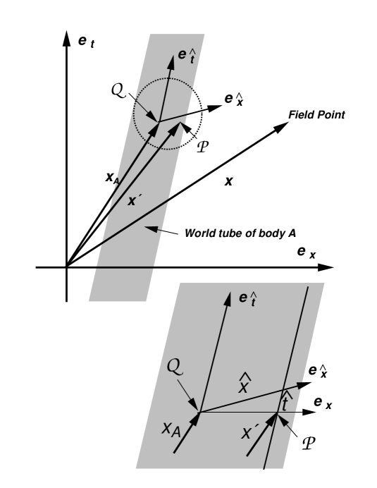
FIG. 1.: Transformation to the local comoving frame of one body. Global harmonic coordinates are $t,x^{j}$; local coordinates are ${\hat{t}},{\hat{x}}^{j}$. In local coordinates, the density of the body is assumed to be static and spherically symmetric.

REFERENCES

- [1] C. Cutler, T. A. Apostolatos, L. Bildsten, L. S. Finn, É. E. Flanagan, D. Kennefick, D. M. Marković, A. Ori, E. Poisson, G. J. Sussman, and K. S. Thorne, Phys. Rev. Lett. 70, 2984 (1993).
- [2] M. E. Pati and C. M. Will, Phys. Rev. D 62, 124015 (2000)
- [3] T. Damour and N. Deruelle, Phys. Lett. 87A, 81 (1981).
- [4] T. Damour, in 300 Years of Gravitation, edited by S. W. Hawking and W. Israel (Cambridge University Press, London, 1987), p. 128.
- [5] S. M. Kopeikin, Sov. Astron. 29, 516 (1985).
- [6] L. P. Grishchuk and S. M. Kopeikin, In Relativity in Celestial Mechanics and Astrometry, edited by J. Kovalevsky and V. A. Brumberg (Reidel, Dordrecht, 1986), p. 19.
- [7] L. Blanchet, G. Faye and B. Ponsot, Phys. Rev. D 58, 124002 (1998).
- [8] Y. Itoh, T. Futamase, and H. Asada, Phys. Rev. D 63, 064038 (2001).
- [9] C. W. Misner, K. S. Thorne, and J. A. Wheeler, Gravitation (Freeman Publishing Co, San Francisco, 1973).
- [10] B. R. Iyer and C. M. Will, Phys. Rev. Lett. 70, 113 (1993).
- [11] B. R. Iyer and C. M. Will, Phys. Rev. D 52, 6882 (1995).
- [12] G. Schäfer, Ann. Phys. (N.Y.) 161, 81 (1985).
- [13] G. Schäfer, Gen. Relativ. Gravit. 18, 255 (1986).
- [14] P. Jaranowski and G. Schäfer, Phys. Rev. D 55, 4712 (1997).
- [15] P. Jaranowski and G. Schäfer, Phys. Rev. D 57, 5948 (1998), ibid. 57, 7274 (1998).
- [16] P. Jaranowski and G. Schäfer, Phys. Rev. D 60, 124003 (1999).
- [17] T. Damour, P. Jaranowski and G. Schäfer, Phys. Rev. D 62, 021501 (2000).
- [18] L. Blanchet and G. Faye, Phys.Lett. 271A, 58 (2000).
- [19] L. Blanchet and G. Faye, Phys. Rev. D 63, 062005 (2001).
- [20] K. S. Thorne, Rev. Mod. Phys. 52, 299 (1980).
- [21] L. Blanchet and G. Faye, J. Math. Phys. 41, 7675 (2000).
- [22] A. Einstein, L. Infeld, and B. Hoffmann, Ann. Math. 39, 65 (1938).
- [23] Y. Itoh, T. Futamase, and H. Asada, Phys. Rev. D 62, 064002 (2000).
- [24] T. Futamase, Phys. Rev. D 32, 2566 (1985); ibid. 36, 321 (1987).
- [25] C. M. Will, Theory and Experiment in Gravitational Physics (Cambridge University Press, Cambridge, 1993).
- [26] R. V. Wagoner and C. M. Will, Astrophys. J. 210, 764 (1976); 215, 984 (1977).
- [27] L. Blanchet and T. Damour, Ann. Inst. Henri Poincaré A, 50, 377 (1989); L. Blanchet and G. Schäfer, Mon. Not. R. Astron. Soc. 239, 845 (1989).
- [28] W. Junker and G. Schäfer, Mon. Not. R. Astron. Soc. 254, 146 (1992).
- [29] L. Blanchet, Phys. Rev. D 47, 4392 (1993).
- [30] In evaluating integrals of second derivatives of , it is important to use the fact that .