Algebraic approach to time-delay data analysis for LISA

Abstract

Cancellation of laser frequency noise in interferometers is crucial for attaining the requisite sensitivity of the triangular 3-spacecraft LISA configuration. Raw laser noise is several orders of magnitude above the other noises and thus it is essential to bring it down to the level of other noises such as shot, acceleration, etc. Since it is impossible to maintain equal distances between spacecrafts, laser noise cancellation must be achieved by appropriately combining the six beams with appropriate time-delays. It has been shown in several recent papers that such combinations are possible. In this paper, we present a rigorous and systematic formalism based on algebraic geometrical methods involving computational commutative algebra, which generates in principle all the data combinations cancelling the laser frequency noise. The relevant data combinations form the first module of syzygies, as it is called in the literature of algebraic geometry. The module is over a polynomial ring in three variables, the three variables corresponding to the three time-delays around the LISA triangle. Specifically, we list several sets of generators for the module whose linear combinations with polynomial coefficients generate the entire module. We find that this formalism can also be extended in a straight forward way to cancel Doppler shifts due to optical bench motions. The two modules are infact isomorphic.

We use our formalism to obtain the transfer functions for the six beams and for the generators. We specifically investigate monochromatic gravitational wave sources in the LISA band and carry out the maximisiation over linear combinations of the generators of the signal-to-noise ratios with the frequency and source direction angles as parameters.

I Introduction

Breakthroughs in modern technology have made possible the construction of extremely large interferometers both on ground and in space for the detection and observation of gravitational waves (GW). Several ground based detectors are being constructed around the globe; these are the projects, LIGO, VIRGO, GEO, TAMA and AIGO of building interferometers whose armlengths will be of the order of kilometers. These detectors will operate in the high frequency range of GW of $\sim 10$ Hz to a few kHz. A natural limit occurs on decreasing the lower frequency cut-off of $10$ Hz because it is not practical to increase the armlengths on ground and also because of the gravity gradient noise which is difficult to eliminate below $10$ Hz. Thus, the ground based interferometers will not be sensitive below the limiting frequency of $\sim 10$ Hz. But on the otherhand, there exist in the cosmos, interesting astrophysical GW sources which emit GW below this frequency such as the galactic binaries, massive and supermassive blackhole binaries etc. If we wish to observe these sources, we need to go to lower frequencies. The solution is to build an interferometer in space, where such noises will be absent and allow the detection of GW in the low frequency regime. LISA - Laser Interferometric Space Antenna - is a proposed mission which will use coherent laser beams exchanged between three identical spacecrafts forming a giant (almost) equilateral triangle of side $5\times 10^{6}$ kilometers to observe and detect low frequency cosmic GW. The ground based detectors and LISA complement each other in the observation of GW in an essential way, analogous to the optical, radio, X-ray, $\gamma$-ray etc., observations do for the electromagnetic waves. As these detectors begin to operate, a new era of Gravitational Astronomy is on the horizon and a radically different view of the universe is expected to be revealed.

In ground based detectors the arms are chosen to be of equal length so that the laser light experiences identical delay in each arm of the interferometer. This arrangement precisely cancels the laser frequency/phase noise at the photodetector. This cancellation of noise is crucial since the raw laser noise is orders of magnitude larger than other noises in the interferometer. The required sensitivity of the instrument can thus only be achieved by near exact cancellation of the laser frequency noise. However, in LISA it is impossible to achieve equal distances between spacecrafts and the laser noise cannot be cancelled in an obvious manner. In LISA, six data streams arise from the exchange of laser beams between the three spacecrafts - it is not possible to bounce laser beams between different spacecrafts, as is done in ground based detectors; a scheme analogous to the RF transponder scheme is used as was done in the early experiments for detecting GW by Doppler tracking a spacecraft from Earth. Several schemes, some quite elaborate, have been proposed [1, 2] which combine the recorded data by suitable time-delays corresponding to the three armlengths of the giant triangular interferometer. These schemes have data combinations of six or at most eight data points which give respectively a six and eight pulse response of GW and also show how other data combinations can be obtained by linear superposition.

Galactic and extragalactic binaries are important sources in the LISA frequency band. Their abundance and resulting spectral amplitude has been estimated using the population synthesis by various authors[PBDH [8]-NYPZ [15]]. In the lower frequency range ($\leq 1$ mHz) there are a large number of such sources in each of the frequency bins. This makes it impossible to resolve an individual source which results in a stochastic GW background. It has been also proposed that the galactic halo MACHOs such as white dwarfs and blackholes ( with mass $\sim 0.5~{}M_{\odot}~{}$) can also produce stochastic GW background[WH [16]-HSR [18]]. In a recent work, Tinto at. al[19] have used Doppler delayed beams for discriminating the stochastic background from the instrumental noise. The angular resolution of the LISA is restricted because it is an all-sky monitoring detector with quadrupole beam pattern, however, the angular resolution can be achieved by the relative amplitude and phases of the two polarisations and Doppler modulation of the beams due to the motion of LISA around the sun[21, 20].

We start with the fundamental papers by the JPL team [1, 2, 3] where idea of delayed data combinations was first proposed. Here we present a systematic method based on modules over polynomial rings, which not only reproduces the previously obtained results, but guarantees all the data combinations which cancel the laser noise. The data combinations in the case of laser frequency noise consist of the six suitably delayed data streams, the delays being integer multiples of the light travel times between spacecrafts, which can be conveniently expressed in terms of polynomials in the three delay operators $E_{1},E_{2},E_{3}$ corresponding to the light travel time along the three arms. The laser noise cancellation condition puts three constraints on the six polynomials of the delay operators corresponding to the six data streams. The problem therefore consists of finding six tuples of polynomials which satisfy the laser noise cancellation constraints. These polynomial tuples form a module called in the literature, the module of syzygies. There exist standard methods for obtaining the module, by that we mean, methods for obtaining the generators of the module so that the linear combinations of the generators generate the entire module. Three constraints on six tuples of polynomials do not lead to three generators as naive reasoning might suggest. Here we are dealing with modules rather than vector spaces and the rules are different. The procedure first consists of obtaining a Groebner basis for the ideal generated by the coefficients appearing in the constraints. This ideal is in the polynomial ring in $E_{1},E_{2},E_{3}$ over the domain of rational numbers (or integers if one gets rid of the denominators). To obtain the Groebner basis for the ideal, one may use the Buchberger algorithm or use a package such as Mathematica. From the Groebner basis there is a standard way to obtain a generating set for the required module. All of this procedure has been described in the literature [4, 5]. We thus obtain seven generators for the module. However, the method does not guarantee a minimal set and we find that a generating set of 4 polynomial six tuples suffice to generate the required module. Alternatively, we can obtain generating sets by using the software Macaulay 2. It gives us a a Groebner basis for the module consisting of five generators and another generating set consisting of six elements. The importance of obtaining more data combinations is evident: they provide the necessary redundancy - different data combinations produce different transfer functions for GW and so specific data combinations could be optimal for given astrophysical source parameters in the context of maximising signal-to-noise (SNR), detection probability, improving parameter estimates etc.

The scheme we have described above can also be extended in a straight forward way to include optical bench motions. There are now twelve Doppler streams of data and we apply the above scheme to cancel the noise due to optical bench drift and laser frequency noise. The six extra streams can be combined two by two by subtracting one stream from the other to obtain three streams in which the frequency shifts in the optical fibers are cancelled. Thus we have only nine streams to contend with and now the module consists of nine tuples of polynomials on which six linear constraints are imposed. We show that the problem can be solved in the terms of the previous one where the three extra polynomials are written in terms of the six tuple polynomials which are solutions to the laser frequency noise cancellation problem. Thus the solution to the first problem extends easily to the second.

Finally, we apply our formalism to a class of important astrophysical sources, but relatively simple to analyse, namely, monochromatic GW sources. We maximise the SNR for such sources over much of the module of data combinations by considering linear combinations of the generators of the module with the coefficients being real numbers. Strictly speaking one must take polynomials as the coefficients so that the maximisation extends to the entire module, but we find that even this simplifying assumption yields satisfactory results. We present the maximised SNR as a function of frequency over the data combinations.

We organise the paper in the following manner: In the section II, we present the six raw data streams obtained with the laser phase noise and formulate the conditions for the laser phase noise cancellation. We also obtain difference equations which should be satisfied by the time-delay operators for cancelling the laser noise. The solutions for the noise cancellation combinations can be represented as the modules syzygies over the polynomial ring using standard methods of algebraic geometry described in the section III. First a Groebner basis for the ideal is obtained. From the Groebner basis the generators for the module of syzygies can be computed. Several sets of generators have been obtained for this module. In the subsection III B this approach is extended to cancel the acceleration noise of the optical benches. In the section IV we compute the detector response for the GW signal and obtain transfer functions for the six elementary beams. In the section V, first, we determine the effective noise for each generator by taking shotnoise and acceleration noise of the proof masses into account, which do not cancel out in the combinations. We obtain SNRs for monochromatic sources and maximise the SNR over the allowed data combinations that cancel the laser frequency noise.

II Time Delayed Data and the Difference Equation

A Time-delayed Data

We label the spacecrafts as 1,2 and 3. Let $L_{1},L_{2},L_{3}$ be the lengths of the arms (sides of the triangle) where $L_{3}$ is the distance between spacecrafts 1 and 2; and so on by cyclic rotation of indices (see figure 1). Each spacecraft has a laser which is

• used to send beams to the other two spacecrafts, and,

• used as a local oscillator to produce a beat signal with the incoming beams from the other two spacecrafts.

The data are recorded as fractional Doppler shifts. These fractional Doppler shifts can occur due to the GW signal and the noise. Here we will be concerned with the laser frequency noise only. More precisely, if $\nu_{0}$ is the central frequency of the laser and the frequency fluctuation of the laser on spacecraft $i$ at time $t$ is $\Delta\nu_{i}(t)$, then the fractional frequency fluctuation $C_{i}(t)$ is given by,

$$C_{i}(t)={\Delta\nu_{i}(t)\over\nu_{0}}.$$ (1)

The six streams of Doppler data are obtained from the $C_{i}(t)$ by combining them suitably with their time delayed copies, where the time delays are just the light travel times between the three spacecrafts. We adopt the following notation for the six streams: we divide the six streams into two sets $U^{i}$ and $V^{i}$ where, $i=1,2,3$ of three streams each. $U^{i}$ and $V^{i}$ can be regarded as 3 component vectors ${\bf U}$ and ${\bf V}$ respectively. Also we denote the time-delayed data in arm $k$, $k=1,2,3,$ by the shift operator $E_{k}$ whose action on a function $f(t)$ is described by the equation:

FIG. 1.: LISA Geometry

$$E_{k}f(t)=f(t-L_{k}),$$ (2)

where we have chosen units in which the speed of light is unity. The six streams are:

$$U^{1} = E_{2}C_{3}-C_{1},$$ (3)

$$U^{2} = E_{3}C_{1}-C_{2},$$ (4)

$$U^{3} = E_{1}C_{2}-C_{3},$$ (5)

$$V^{1} = C_{1}-E_{3}C_{2},$$ (6)

$$V^{2} = C_{2}-E_{1}C_{3},$$ (7)

$$V^{3} = C_{3}-E_{2}C_{1}.$$ (8)

Thus explicitly we have, $U^{1}(t)=C_{3}(t-L_{2})-C_{1}(t)$ etc. $U^{1}(t)$ is the data stream obtained by beating the laser beam transmitted by spacecraft 3 to spacecraft 1 measured at time $t$ at spacecraft 1; and so on by cyclic rotation. Similarly $-V^{1}(t)=C_{2}(t-L_{3})-C_{1}(t)$ is the laser beam emitted by spacecraft 2 and received and beaten with the laser at spacecraft 1 at time $t$. If we label the spacecrafts in a counter-clockwise (positive sense) fashion, then the beams $U^{i}$ travel in the positive sense while the beams $V^{i}$ travel in the negative sense.

The goal of the analysis is to add suitably delayed beams together so that the net result is zero. This amounts to seeking data combinations which cancel the laser frequency noise. In the notation/formalism that we have invoked, the delay is obtained by applying the operators $E_{k}$ to the beams $U^{i}$ and $V^{i}$. A delay of $k_{1}L_{1}+k_{2}L_{2}+k_{3}L_{3}$ is represented by the operator $E_{1}^{k_{1}}E_{2}^{k_{2}}E_{3}^{k_{3}}$ acting on the data, where $k_{1},k_{2}$ and $k_{3}$ are integers. In general a polynomial in $E_{k}$, which is a polynomial in three variables, applied to say $U^{1}$ combines the same data stream $U^{1}(t)$ with different time-delays of the form $k_{1}L_{1}+k_{2}L_{2}+k_{3}L_{3}$. This notation conveniently rephrases the problem. One must find six polynomials say $p_{i}(E_{1},E_{2},E_{3}),\ q_{i}(E_{1},E_{2},E_{3}),\ i=1,2,3$ such that:

$$\sum_{i=1}^{3}p_{i}V^{i}+q_{i}U^{i}=0.$$ (9)

Cancellation of the laser noise is implicit in the above equation.

B The Difference Equation for Shift Operators

It is convenient to express eq. (8) in matrix form. This allows us to obtain a matrix operator equation whose solutions are ${\bf p}$ and ${\bf q}$ where we have now written $p^{i}$ and $q^{i}$ as column vectors. We can similarly express $U^{i},V^{i},C^{i}$ as column vectors ${\bf U},{\bf V},{\bf C}$ respectively. In matrix form eq. (8) become:

$${\bf V}={\bf\mu}^{T}\ {\bf C},~{}~{}~{}~{}~{}~{}~{}{\bf U}=-{\bf\mu}\ {\bf C},$$ (10)

where, ${\bf\mu}$ is a $3\times 3$ matrix given by,

$${\bf\mu}=\left(\begin{array}[]{ccc}1&0&-E_{2}\\ -E_{3}&1&0\\ 0&-E_{1}&1\end{array}\right)\,.$$ (11)

The exponent ‘T’ represents the transpose of the matrix. The eq. (9) becomes:

$$({\bf\mu}{\bf p}-{\bf\mu}^{T}{\bf q})^{T}\ {\bf C}=0\,.$$ (12)

where we have taken care to put ${\bf C}$ on the right of the operators. Since the above equation must be satisfied for arbitrary ‘data’ ${\bf C}$, we obtain a matrix equation for the shift operators:

$${\bf\mu}{\bf p}={\bf\mu}^{T}{\bf q}\,.$$ (13)

The solutions to eq. (13) are ${\bf p},{\bf q}$ which are column vectors of polynomials in the shift operators $E_{k}$. Note that since the $E_{k}$ are just shift operators, they commute, so the order in writing these operators is unimportant. In mathematical terms, the polynomials form a commutative ring.

We can formally solve for ${\bf p}$ since the matrix ${\bf\mu}$ is invertible. However, $\det{\bf\mu}=1-E_{1}E_{2}E_{3}$ appears in the denominator on the R.H.S., which leads to the division by polynomials in $E_{k}$. This may seem hard to interpret. But we can pull this factor to the L. H. S. to ‘rationalise’ the expressions. Then we obtain,

$$\Delta{\bf p}={\bf A}\ {\bf q}\,,$$ (14)

where ${\bf A}={\bf\mu}_{adj}{\bf\mu}^{T}$ and ${\bf\mu}_{adj}$ is the adjoint of ${\bf\mu}$. The operator $\Delta=1-E_{1}E_{2}E_{3}$ is the usual difference operator that appears in finite differences and difference equations. The quantity $E_{1}E_{2}E_{3}$ plays a central role in determining the natural time-step for the problem, namely, $s=L_{1}+L_{2}+L_{3}$; which is nothing but the light travel time around the perimeter of the LISA triangle. $\Delta$ is just the difference corresponding to this time-step.

Explicitly, using (11) the matrix ${\bf A}$ is given by:

$${\bf A}=\left(\begin{array}[]{ccc}1-E_{2}^{2}&E_{1}E_{2}-E_{3}&E_{2}(1-E_{1}^{2})\\ (1-E_{2}^{2})E_{3}&1-E_{3}^{2}&E_{2}E_{3}-E_{1}\\ E_{3}E_{1}-E_{2}&E_{1}(1-E_{3}^{2})&1-E_{1}^{2}\end{array}\right)\,.$$ (15)

The equations display a cyclic symmetry in the indices $1,2,3$ which is also apparent in the matrix ${\bf A}$. The cyclic symmetry results from the nature of the problem since we are free to choose the labeling of the three space-crafts. In the matrix ${\bf A}$ we must also change the rows/columns consistently performing the cyclic change of the indices. The cyclic symmetry is further carried over to the solutions $({\bf p},{\bf q})$.

The integration of the eq. (14) can be carried out in time-steps of $s$. The integration is immediate if we operate the eq. (14) on ${\bf V}$. We first need to take the transpose of eq. (14) and then operate on ${\bf V}$. We then obtain:

$$\Delta{\bf p}^{T}{\bf V} = {\bf q}^{T}{\bf A}^{T}\ {\bf V}$$ (16)

$$= {\bf q}^{T}({\bf\mu}_{adj}{\bf\mu}^{T})^{T}\ {\bf V}$$ (17)

$$= {\bf q}^{T}{\bf\mu}\Delta\ {\bf C}$$ (18)

$$= -\Delta{\bf q}^{T}\ {\bf U}\,,$$ (19)

which gives,

$$\Delta({\bf p}^{T}\ {\bf V}+{\bf q}^{T}\ {\bf U})=0.$$ (20)

This equation immediately integrates to,

$$({\bf p}^{T}\ {\bf V}+{\bf q}^{T}\ {\bf U})(t+ns)=({\bf p}^{T}\ {\bf V}+{\bf q}^{T}\ {\bf U})(t),$$ (21)

where $n$ is an integer. If we arbitrarily set $t=0$ and if $({\bf p}^{T}\ {\bf V}+{\bf q}^{T}\ {\bf U})(0)=0$, then $({\bf p}^{T}\ {\bf V}+{\bf q}^{T}\ {\bf U})(ns)=0$.

It is not clear to us, how the above solution would be useful physically, but we present it as an interesting outcome. However, the main problem is of seeking solutions $({\bf p},{\bf q})$ to eq.(13). This problem and its solution we discuss in the next section.

III The modules of syzygies

Several solutions have been exhibited in [1, 2] to eq.(13). The solutions have the characteristic property that the $\det{\bf\mu}$ cancels on both sides leading to polynomial vectors ${\bf p}$ and ${\bf q}$. We reproduce here the solutions obtained in previous works. The solution $\zeta$ is given by ${\bf p}^{T}={\bf q}^{T}=(E_{1},E_{2},E_{3})$. The solution $\alpha$ is described by ${\bf p}^{T}=(1,E_{3},E_{1}E_{3})$ and ${\bf q}^{T}=(1,E_{1}E_{2},E_{2})$. The solutions $\beta$ and $\gamma$ are obtained from $\alpha$ by cyclically permuting the indices of $E_{k},{\bf p}$ and ${\bf q}$. These solutions as realised in earlier works are important, because they consist of polynomials with lowest possible degrees and thus are simple. Other solutions containing higher degree polynomials can be generated conveniently from these solutions. Linear combinations of these solutions are also solutions to the given system of equations. But it is not clear that this procedure generates all the solutions. In particular, $\zeta$ cannot be generated from the set $\alpha,\ \beta$ and $\gamma$, where generating a data combination means writing it as a linear combination of the elements belonging to the generating set.

The basic reason, as mentioned earlier, is that we do not have a vector space here. Three independent constraints on a six tuple do not produce a space which is necessarily generated by three basis elements. This conclusion would follow if the solutions formed a vector space but they do not. The polynomial six-tuple ${\bf p},{\bf q}$ can be multiplied by polynomials in $E_{1},E_{2},E_{3}$ (scalars) which do not form a field. So that the inverse in general does not exist within the ring of polynomials. We therefore have a module over the ring of polynomials in the three variables $E_{1},E_{2},E_{3}$.

In this section we present the general methodology for obtaining the solutions to (13). The method is illustrated by applying it to equations (13). In the next subsection we consider the more general problem of optical bench motions as well. The optical bench motion noise can also be eliminated using the same method.

A Cancellation of laser frequency noise

There are three linear constraints on the polynomials given by the equations (13). Since the equations are linear the solutions space is a submodule of the module of six-tuples of polynomials. The module of six-tuples is a free module, i.e. it has six basis elements that not only generate the module but are linearly independent. A natural choice of the basis is $f_{i}=(0,...,1,...,0)$ with 1 in the $i$-th place and 0 everywhere else; $i$ runs from 1 to 6. The definitions of generation (spanning) and linear independence are the same as that for vector spaces. A free module is essentially like a vector space. But our interest lies in its submodule which need not be free and need not have just three generators as it would seem if we were dealing with vector spaces.

The problem at hand is of finding the generators of this submodule i.e. any element of the module should be expressible as a linear combination of the generating set. In this way the generators are capable of spanning the full module or generating the module. We examine the eq.(13) explicitly componentwise:

$$p_{1}-q_{1}+E_{3}q_{2}-E_{2}p_{3} = 0,$$ (22)

$$p_{2}-q_{2}+E_{1}q_{3}-E_{3}p_{1} = 0,$$ (23)

$$p_{3}-q_{3}+E_{2}q_{1}-E_{1}p_{2} = 0.$$ (24)

The first step is to use Gaussian elimination to obtain $p_{1}$ and $p_{2}$ in terms of $p_{3},q_{1},q_{2},q_{3}$. We then obtain:

$$p_{1} = q_{1}-E_{3}q_{2}+E_{2}p_{3},$$ (25)

$$p_{2} = q_{2}-E_{1}q_{3}+E_{3}p_{1}$$ (26)

$$= E_{3}q_{1}+(1-E_{3}^{2})q_{2}-E_{1}q_{3}+E_{2}E_{3}p_{3},$$ (27)

and then substitute these values in the third equation to obtain a linear implicit relation between $p_{3},q_{1},q_{2},q_{3}$. We then have:

$$(E_{1}E_{2}E_{3}-1)p_{3}+(E_{1}E_{3}-E_{2})q_{1}+E_{1}(1-E_{3}^{2})q_{2}+(1-E_{1}^{2})q_{3}=0.$$ (28)

Obtaining solutions to (28) amounts to solving the problem since the the remaining polynomials $p_{1},p_{2}$ have been expressed in terms of $p_{3},q_{1},q_{2},q_{3}$ in (27).

The solutions to (28) form the first module of syzygies of the coefficients in the eq. (28), namely,
$E_{1}E_{2}E_{3}-1,E_{1}E_{3}-E_{2},E_{1}(1-E_{3}^{2}),1-E_{1}^{2}$. The generators of this module can be obtained from standard methods available in the literature. We briefly outline the method given in the books by Becker et al. [4] and Kreuzer and Robbiano [5] below. The details have been included in the Appendix.

1 Groebner basis

The first step is to obtain the Groebner basis for the ideal ${\cal U}$ generated by the coefficients:

$$u_{1}=E_{1}E_{2}E_{3}-1,~{}~{}u_{2}=E_{1}E_{3}-E_{2},~{}~{}u_{3}=E_{1}(1-E_{3}^{2}),~{}~{}u_{4}=1-E_{1}^{2}.$$ (29)

The ideal ${\cal U}$ consists of linear combinations of the form $\sum v_{i}u_{i}$ where $v_{i}$, $i=1,...,4$ are polynomials in the ring ${\cal Q}[E_{1},E_{2},E_{3}]$ where ${\cal Q}$ is the field of rational numbers. There can be several sets of generators for ${\cal U}$. A Groebner basis is a set of generators which is ‘small’ in a specific sense.

There are several ways to look at the theory of Groebner basis. One way is, suppose we are given polynomials $g_{1},g_{2},...,g_{m}$ in one variable over say ${\cal Q}$ and we would like to know whether another polynomial $f$ belongs to the ideal generated by the $g$’s. A good way to decide the issue would be to first compute the gcd (greatest common divisor) $g$ of $g_{1},g_{2},...,g_{m}$ and checking whether $f$ is a multiple of $g$. One can achieve this by doing the long division of $f$ by $g$ and checking whether the remainder is zero. All this is possible because ${\cal Q}[x]$ is a Euclidean domain and also a principle ideal domain (PID) wherein any ideal is generated by a single element. Therefore we have essentially just one polynomial - the gcd - which generates the ideal generated by $g_{1},g_{2},...,g_{m}$. The ring of integers or the ring of polynomials in one variable over any field are examples of PIDs whose ideals are generated by single elements. However, when we consider more general rings (not PIDs) like the one we are dealing with here, we do not have a single gcd but a set of several polynomials which generates an ideal in general. A Groebner basis of an ideal can be thought of as a generalisation of the gcd. In the univariate case, the Groebner basis reduces to the gcd.

Groebner basis theory generalises these ideas to multivariate polynomials which are neither Euclidean rings nor PIDs. Since there is in general not a single generator for an ideal, Groebner basis theory comes up with the idea of dividing a polynomial with a set of polynomials, the set of generators of the ideal, so that by successive divisions by the polynomials in this generating set of the given polynomial, the remainder becomes zero. Clearly, every generating set of polynomials need not possess this property. Those special generating sets that do possess this property (and they exist!) are called Groebner bases. In order for a division to be carried out in a sensible manner, an order must be put on the ring of polynomials, so that the final remainder after every division is strictly smaller than each of the divisors in the generating set. A natural order exists on the ring of integers or on the polynomial ring ${\cal Q}(x)$; the degree of the polynomial decides the order in ${\cal Q}(x)$. However, even for polynomials in two variables there is no natural order apriori ( Is $x^{2}+y$ greater or smaller than $x+y^{2}$? ). But one can, by hand as it were, put a order on such a ring by saying $x>>y$, where $>>$ is an order, called the lexicographical order. We follow this type of order, $E_{1}>>E_{2}>>E_{3}$ and ordering polynomials by considering their highest degree terms. It is possible to put different orderings on a given ring which then produces different Groebner bases. Clearly, a Groebner basis must have ‘small’ elements so that division is possible and every element of the ideal when divided by the Groebner basis elements leaves zero remainder, i.e. every element modulo the Groebner basis reduces to zero.

In the literature, there exists a well-known algorithm called the the Buchberger algorithm which may be used to obtain the Groebner basis for a given set of polynomials in the ring. So a Groebner basis of ${\cal U}$ can be obtained from the generators $u_{i}$ given in eq.(29) using this algorithm. It is essentially again a generalisation of the usual long division that we perform on univariate polynomials. More conveniently, we prefer to use the wellknown ‘Mathematica’ package. Mathematica yields a 3 element Groebner basis ${\cal G}$ for ${\cal U}$:

$${\cal G}=\{E_{3}^{2}-1,E_{2}^{2}-1,E_{1}-E_{2}E_{3}\}\,.$$ (30)

One can easily check that all the $u_{i}$ of eq.(29) are linear combinations of the polynomials in ${\cal G}$ and hence ${\cal G}$ generates ${\cal U}$. One also observes that the elements look ‘small’ in the order mentioned above. However, one can satisfy oneself that ${\cal G}$ is a Groebner basis by using the standard methods available in the literature. One method consists of computing the S-polynomials (see Appendix A) for all the pairs of the Groebner basis elements and checking whether these reduce to zero modulo ${\cal G}$.

This Groebner basis of the ideal ${\cal U}$ is then used to obtain the generators for the module of syzygies.

2 Generating set for the module of syzygies

The generating set for the module is obtained by further following the procedure in the literature [4, 5]. The details are given in the Appendix specifically for our case. We obtain 7 generators for the module. These generators do not form a minimal set and there are relations between them; in fact this method does not guarantee a minimum set of generators. These generators can be expressed as linear combinations of $\alpha,\beta,\gamma,\zeta$ and also in terms of $X^{(1)},X^{(2)},X^{(3)},X^{(4)}$ given below in eq.(34). The importance in obtaining the 7 generators is that the standard theorems guarantee that these 7 generators do infact generate the required module. Therefore from this proven set of generators we can check whether a particular set is infact a generating set. We present several generating sets below:

Alternatively, we may use a software package called ‘Macaulay 2’ which calculates the generators given the the equations (24). Using Macaulay 2, we obtain six generators. Again, Macaulay’s algorithm does not yield a minimal set; we can express the last two generators in terms of the first four. Below we list this smaller set of four generators in the order $X=(p_{1},p_{2},p_{3},q_{1},q_{2},q_{3})$:

$$X^{(1)} = (E_{1}E_{3}-E_{2},0,E_{3}^{2}-1,0,E_{2}E_{3}-E_{1},E_{3}^{2}-1),$$ (31)

$$X^{(2)} = (E_{1},E_{2},E_{3},E_{1},E_{2},E_{3}),$$ (32)

$$X^{(3)} = (1,E_{3},E_{1}E_{3},1,E_{1}E_{2},E_{2}),$$ (33)

$$X^{(4)} = (E_{1}E_{2},1,E_{1},E_{3},1,E_{2}E_{3}).$$ (34)

Note that the last three generators are just $X^{(2)}=\zeta,X^{(3)}=\alpha,X^{(4)}=\beta$. But there is an extra generator $X^{(1)}$ needed to generate all the solutions.

Another set of generators which could be useful for further work is a Groebner basis of a module. The concept of a Groebner basis of an ideal can be extended to that of a Groebner basis of a submodule of $(K[x_{1},x_{2},...,x_{n}])^{m}$ where $K$ is a field, since a module over the polynomial ring can be considered as generalisation of an ideal in a polynomial ring. Just as in the case of an ideal, a Groebner basis for a module is a generating set with special properties. For the module under consideration we obtain a Groebner basis using Macaulay 2 :

$$G^{(1)} = (E_{1},E_{2},E_{3},E_{1},E_{2},E_{3}),$$ (35)

$$G^{(2)} = (E_{1}E_{3}-E_{2},0,E_{3}^{2}-1,0,E_{2}E_{3}-E_{1},E_{3}^{2}-1),$$ (36)

$$G^{(3)} = (E_{1}E_{2},1,E_{1},E_{3},1,E_{2}E_{3}),$$ (37)

$$G^{(4)} = (1,E_{3},E_{1}E_{3},1,E_{1}E_{2},E_{2}),$$ (38)

$$G^{(5)} = (E_{3}(E_{1}^{2}-1),1-E_{3}^{2},0,0,1-E_{1}^{2},E_{1}(E_{3}^{2}-1)).$$ (39)

Note that in this Groebner basis $G^{(1)}=\zeta=X^{(2)},G^{(2)}=X^{(1)},G^{(3)}=\beta=X^{(4)},G^{(4)}=\alpha=X^{(3)}$. Only $G^{(5)}$ is the new generator.

Another set of generators are just $\alpha,\beta,\gamma$ and $\zeta$. This can be checked using Macaulay 2 or one can relate $\alpha,\beta,\gamma$ and $\zeta$ to the generators $X^{(A)},A=1,2,3,4$ by polynomial matrices. In the Appendix, we express the 7 generators we obtained following the literature, in terms of $\alpha,\beta,\gamma$ and $\zeta$. Also we express $\alpha,\beta,\gamma$ and $\zeta$ in terms of $X^{(A)}$. This proves that all these sets generate the required module of syzygies.

The question now arises as to which set of generators we should choose which facilitates further analysis. The analysis is simplified if we choose a smaller number of generators. Also we would prefer low degree polynomials to appear in the generators so as to avoid cancellation of leading terms in the polynomials. By these two criteria we may choose, $X^{(A)}$ or $\alpha,\beta,\gamma,\zeta$. Among these two sets of generators, we arbitrarily make the choice of $X^{(A)}$.

B Cancellation of noise from moving optical benches

The work done in [1, 2] can be conveniently reexpressed in our formulation and leads to further insights into the problem.

There are two optical benches on each space-craft which have random velocities and are connected by optical fibers. The random velocities of the optical benches and the delay in the optical fibers are measured as further Doppler shifts apart from other noise and the GW signal. Since we are interested in the cancellation of laser frequency noise and motion of the optical benches, we write expressions for the beams containing only these quantities. The Doppler beams will of course contain other effects arising from shot noise, GW signal, motion of proof masses etc., but we will not write them in the expressions for the Doppler data because they are not relevant to the problem we are interested in. We follow the notations of [1, 2]. The quantities pertaining to the left bench will be unstarred while that for the right bench are starred. There are now twelve Doppler data streams which need to be combined in an appropriate manner in order to cancel the noise from the laser as well as from the motion of the optical benches. The fractional frequency fluctuations of laser on the left optical bench $i$ are denoted by $C_{i}$ and on the right optical bench $i^{*}$ by $C_{i}^{*}$, the random velocities of the benches ${\bf V}_{i},{\bf V}_{i}^{*}$ and $\eta_{i}$ the frequency shifts in the optical fibers connecting the optical benches in space-craft $i$. We then have the following expressions for the four data streams pertaining to space-craft $1$:

$$U^{1} = E_{2}(C_{3}-{\bf{\hat{n}}}_{2}\cdot{\bf V}_{3})-({\bf{\hat{n}}}_{2}\cdot{\bf V}^{*}_{1}+C_{1}^{*}),$$ (40)

$$V^{1} = -E_{3}(C_{2}^{*}+{\bf{\hat{n}}}_{3}\cdot{\bf V}_{2}^{*})+(C_{1}-{\bf{\hat{n}}}_{3}\cdot{\bf V}_{1}),$$ (41)

$$z_{1} = C_{1}-C_{1}^{*}+\eta_{1}-2{\bf{\hat{n}}}_{3}\cdot{\bf V}_{1}\,,$$ (42)

$$z_{1}^{*} = C_{1}^{*}-C_{1}+\eta_{1}+2{\bf{\hat{n}}}_{2}\cdot{\bf V}_{1}^{*}\,.$$ (43)

The other eight data streams on space crafts 2 and 3 are obtained by cyclic permutations of the indices in the above equations. Here ${\bf{\hat{n}}}_{2}$ denotes a unit vector in the direction from space-craft 1 to space-craft 3 and the remaining unit vectors ${\bf{\hat{n}}}_{3}$ and ${\bf{\hat{n}}}_{1}$ are obtained by cyclically permutating the indices.

We find that the twelve Doppler data streams depend only on the particular combinations $C_{1}-{\bf{\hat{n}}}_{3}\cdot{\bf V}_{1}$ and $C_{1}^{*}+{\bf{\hat{n}}}_{2}\cdot{\bf V}_{1}^{*}$ and their cyclic permutations. We define these combinations as ${\tilde{C}}_{1}$ and ${\tilde{C}}_{1}^{*}$ respectively, i.e.:

$${\tilde{C}}_{1} = C_{1}-{\bf{\hat{n}}}_{3}\cdot{\bf V}_{1}\,,$$ (44)

$${\tilde{C}}_{1}^{*} = C_{1}^{*}+{\bf{\hat{n}}}_{2}\cdot{\bf V}_{1}^{*}\,,$$ (45)

and also their cyclic permutations. Then the expressions for the data streams simplify considerably. We write the expressions for the data streams corresponding to space-craft 1. Others are obtained as before by cyclic permutations.

$$U^{1} = E_{2}{\tilde{C}}_{3}-{\tilde{C}}_{1}^{*}\,,$$ (46)

$$V^{1} = -E_{3}{\tilde{C}}_{2}^{*}+{\tilde{C}}_{1}\,,$$ (47)

$$Z^{1} = {1\over 2}(z_{1}-z_{1}^{*})$$ (48)

$$= {\tilde{C}}_{1}-{\tilde{C}}_{1}^{*}\,.$$ (49)

The new variables $Z^{i}$ have been defined which automatically cancel the $\eta_{i}$. Also we note that the $U^{i},V^{i}$ have the same form as in eq. (8), except that the $C_{i}$ are replaced by the ${\tilde{C}}_{i}$ which account for the motions of the optical benches.

The noise cancellation condition now becomes:

$$p_{i}V^{i}+q_{i}U^{i}+r_{i}Z^{i}=0\,,$$ (50)

where $r_{i}$ are polynomials in $E_{1},E_{2},E_{3}$. Since the above equations should hold for any ${\tilde{C}}_{i},{\tilde{C}}_{i}^{*}$, we obtain the following equations the polynomials $p_{i},q_{i},r_{i}$ must satisfy:

$$p_{1}+E_{3}q_{2}+r_{1} = 0\,,$$ (51)

$$E_{2}p_{3}+q_{1}+r_{1} = 0\,,$$ (52)

$$p_{2}+E_{1}q_{3}+r_{2} = 0\,,$$ (53)

$$E_{3}p_{1}+q_{2}+r_{2} = 0\,,$$ (54)

$$p_{3}+E_{2}q_{1}+r_{3} = 0\,,$$ (55)

$$E_{1}p_{2}+q_{3}+r_{3} = 0\,.$$ (56)

We now have a nine component polynomial vector. The solutions to (56) form another module of syzygies which is related in a simple way to the module obtained in just laser noise cancellation. Eliminating $r_{i}$ from eq. (56) we obtain the same equations for $p_{i}$ and $q_{i}$ as in (24). This enables us to extend the previously obtained generating sets to this module. Thus, thanks to the mapping of $C_{i},(C_{i}^{*})\longrightarrow{\tilde{C}}_{i},({\tilde{C}}_{i}^{*})$, the two modules are isomorphic. We just state the remaining three entries ($r_{1},r_{2},r_{3}$) of the generating sets keeping the same notation. The first set of 4 generators in the order $(r_{1},r_{2},r_{3})$ are:

$$X^{(1)} = (E_{2}(1-E_{3}^{2}),E_{1}(1-E_{3}^{2}),1-E_{3}^{2})\,,$$ (57)

$$X^{(2)} = -(E_{1}+E_{2}E_{3},E_{2}+E_{1}E_{3},E_{3}+E_{1}E_{2})\,,$$ (58)

$$X^{(3)} = -(1+E_{1}E_{2}E_{3},E_{1}E_{2}+E_{3},E_{1}E_{3}+E_{2})\,,$$ (59)

$$X^{(4)} = -(E_{1}E_{2}+E_{3},1+E_{1}E_{2}E_{3},E_{1}+E_{2}E_{3})\,.$$ (60)

In the other generating set, namely, the Groebner basis we need to specify just $G_{5}$ since the other elements are in the previous generating set. Thus,

$$G^{(5)}=(0,(E_{1}^{2}-1)(1-E_{3}^{2}),0).$$ (61)

IV The Detector response

The ripples produced in the spacetime by the gravitational waves as they propagate through the LISA detector are measured as the Doppler shifts in the laser frequency. The measured signals will have the various noises along with the Doppler shift produced by the gravitational radiation. In the last section we have studied various combinations of beams which cancels the laser phase noise and optical bench acceleration noise. In this section we investigate the response of the detector for these combinations. We compute the transfer functions for the generators and also their linear combinations. The laser phase noise and optical bench acceleration noise is then also cancelled for the linear combinations. However, noises such as the shot noise and the acceleration noise of the proof masses do not cancel out. In the following subsections we set up the coordinate system adapted to the LISA geometry and then go on to compute the response of LISA.

A Parameterisation of the interferometer

Figure 1 describes the LISA configuration. We choose a coordinate system in which the LISA triangle is at rest. Although this coordinate system is in motion relative to the usual coordinate systems normally encountered, we will find such a system of coordinates convenient for further analysis, such as computing SNR’s of monochromatic sources etc.

The unit vector $\hat{w}$ connecting the origin and the source is parameterised by the source angular location $(\theta,\ \phi)$, so that

$$\hat{w}\ =\ \left(\begin{array}[]{c}\sin\theta\ \cos\phi\\ \sin\theta\ \sin\phi\\ \cos\theta\end{array}\right)\,,$$ (62)

the transverse plane is spanned by the unit transverse vector $\hat{\theta}$ and $\hat{\phi}$, defined by

$$\hat{\theta}\ =\ \frac{\partial\hat{w}}{\partial\theta},\ \ \ \ \hat{\phi}\ =\ \frac{1}{\sin\theta}\frac{\partial\hat{w}}{\partial\phi}\,.$$ (63)

As the wave propagates through the LISA triangle, the components of the gravitational perturbation can be written as

$$h_{ij}(t,\vec{r})\ =\ h_{+}\left(t-\hat{w}\cdot\vec{r}\right)\left(\theta_{i}\theta_{j}-\phi_{i}\phi_{j}\right)\ +\ h_{\times}\left(t-\hat{w}\cdot\vec{r}\right)\left(\theta_{i}\phi_{j}+\theta_{j}\phi_{i}\right)\,,$$ (64)

where $h_{+}$ and $h_{\times}$ are arbitrary functions describing the two GW amplitudes.

We consider the effect of this perturbation on the light beam traveling between two points A and B. From this we obtain the complete response. Let $\vec{r}_{A}$ and $\vec{r}_{B}$ be the position vectors of points A and B respectively. Then the line element of the spacetime along the beam null ray obeys,

$$0\ =\ dt^{2}-dx^{2}-dy^{2}-dz^{2}+h_{ij}dx^{i}dx^{j},$$ (65)

where the $i,j$ run over space indices only. If $\hat{n}$ is the unit vector directed from A to B, we have

$$dx^{i}\ =\ n^{i}d\lambda\,,$$ (66)

where $\lambda$ is the Euclidean length. The equations (65) can be expressed as,

$$0\ =\ dt^{2}-d\lambda^{2}\left[1-h_{ij}n^{i}n^{j}\right]\,,$$ (67)

or equivalently

$$d\lambda\ =\ dt\left[1+\frac{1}{2}h\left(t-\hat{w}\cdot\vec{r}\right)\right]\,.$$ (68)

From eq. (64) we get

$$h(t)\ =\ h_{+}(t)\xi_{+}(\theta,\phi)+h_{\times}(t)\xi_{\times}(\theta,\phi)\,,$$ (69)

$$\left\{\begin{array}[]{l}\xi_{+}\ =\ (\hat{\theta}\cdot\hat{n})^{2}-(\hat{\phi}\cdot\hat{n})^{2}\\ \xi_{\times}\ =\ 2(\hat{\theta}\cdot\hat{n})(\hat{\phi}\cdot\hat{n})\end{array}\right.\,.$$ (70)

B $h$-sensitivity of one arm

We now apply the above analysis to compute the Doppler response of the laser beam along one arm of the LISA detector. Let the beam start at $t=t_{0}$ from the point $\vec{r}_{A}$ and travel towards the point $\vec{r}_{B}$ and reach it at $t=t_{1}$. Then,

$$\vec{r}(t)\ =\ \vec{r}_{A}+(t-t_{0})\hat{n},\ \ \ \vec{r}(t_{1})\ =\ \vec{r}_{B}\,.$$ (71)

The line element along this path satisfies the equation,

$$d\lambda\ =\ dt\left\{1+\frac{1}{2}h\left[(1-\hat{w}\cdot\hat{n})t-\hat{w}\cdot\vec{r}_{A}+t_{0}\hat{w}\cdot\hat{n}\right]\right\}\,.$$ (72)

The global travel time $t_{1}-t_{0}$ is given by the integral :

$$L\ =\ t_{1}-t_{0}+\frac{1}{2}\int_{t_{0}}^{t_{1}}h\left[t(1-\hat{w}\cdot\hat{n})-\hat{w}\cdot\vec{r}_{A}+t_{0}\hat{w}\cdot\hat{n}\right]dt\,.$$ (73)

It is convenient for many purposes to pursue our analysis in the Fourier domain. We Fourier transform the GW amplitude $h$:

$$h(t)\ =\ \int d\Omega\ \tilde{h}(\Omega)exp(-i\Omega t)\,,$$ (74)

and the travel time can be expressed as,

$$t_{1}-t_{0}\ =\ L-\frac{1}{2}\int d\Omega\tilde{h}(\Omega)\ \int_{t_{0}}^{t_{1}}exp\left[-i\Omega\left(1-\hat{w}\cdot\hat{n}\right)t\right]exp\left[i\Omega\hat{w}\cdot\vec{r}_{A}\right]exp\left[-i\Omega t_{0}\hat{w}\cdot\hat{n}\right]dt\,.$$ (75)

In the zeroth order of the integral, we have $t_{1}-t_{0}\ =L$, and we obtain:

$$t_{1}-t_{0} = L-\frac{1}{2}\int d\Omega\tilde{h}(\Omega)\ exp\left(i\Omega\hat{w}\cdot\vec{r}_{A}\right)exp\left(-i\Omega t_{1}\right)$$ (76)

$$\times \frac{exp\left(i\Omega L\hat{w}\cdot\hat{n}\right)-exp(i\Omega L)}{-i\Omega(1-\hat{w}\cdot\hat{n})}\,.$$ (77)

The phase change over that time interval is $\Phi=\omega(t_{1}-t_{0})$, where $\omega=2\pi\nu_{opt}$ is the optical circular frequency. We can assume that the time $t_{1}$ is the current time and $t_{0}$ the retarded time, so that the phase is $\Phi(t)=\omega(t-t_{0})$:

$$\Phi(t)\ =\ \omega L - \frac{\omega}{2(1-\hat{w}\cdot\hat{n})}\int d\Omega\tilde{h}(\Omega)\ exp\left(i\Omega\hat{w}\cdot\vec{r}_{A}\right)exp\left(-i\Omega t\right)$$ (78)

$$\times \frac{exp\left(i\Omega L\hat{w}\cdot\hat{n}\right)-exp(i\Omega L)}{-i\Omega}\,.$$ (79)

By taking the time derivative, we get the instantaneous frequency,

$$\frac{\delta\nu(t)}{\nu_{opt}}\ =\ \frac{1}{\omega}\ \frac{d\Phi(t)}{dt}\,.$$ (80)

In the time domain and using $\vec{r}_{A}+L\hat{n}\ =\ \vec{r}_{B}$ we finally get,

$$\frac{\delta\nu(t)}{\nu_{opt}}\ =\ \frac{-1}{2(1-\hat{w}\cdot\hat{n})}\left[h\left(t-\hat{w}\cdot\vec{r}_{B}\right)-h\left(t-\hat{w}\cdot\vec{r}_{A}-L\right)\right].$$ (81)

In the Fourier domain we may express this result as:

$$\frac{\widetilde{\delta\nu(\Omega)}}{\nu_{opt}}\ =\ \frac{\tilde{h}(\Omega)}{2(1-\hat{w}\cdot\hat{n})}exp\left[i\Omega(L+\hat{w}\cdot\vec{r}_{A})\right]\left(1-exp\left[-i\Omega L(1-\hat{w}\cdot\hat{n})\right]\right)\,.$$ (82)

C $h$-sensitivity of the elementary Doppler data

In this section we compute the expression for the transfer function for the six elementary beams given in the eq. (8). These beams further can be combined with suitable delays as described in the previous sections for achieving cancellation of laser phase noise.

The Doppler shift being expressed in the Fourier domain as,

$$\frac{\widetilde{\delta\nu(\Omega)}}{\nu_{opt}}\ =\ \tilde{h}_{+}(\Omega)F_{+}(\Omega)+\tilde{h}_{\times}(\Omega)F_{\times}(\Omega)\,,$$ (83)

where $F_{+,\times}(\Omega)$ are transfer functions. We can compute the transfer functions for the combinations $U_{i},\ V_{i}$. We just give below $F_{U_{1};+,\times}$ and $F_{V_{1};+,\times}$; the others are obtained by cyclic permutations:

$$F_{U_{1};+,\times} = \frac{e^{i\Omega\left(\hat{w}\cdot\vec{r}_{3}+L_{2}\right)}}{2\left(1+\hat{w}\cdot\hat{n}_{2}\right)}\ \left(1-e^{-i\Omega L_{2}\left(1+\hat{w}\cdot\hat{n}_{2}\right)}\right)\xi_{2;+,\times}\,,$$ (84)

$$F_{V_{1};+,\times} = -\frac{e^{i\Omega\left(\hat{w}\cdot\vec{r}_{2}+L_{3}\right)}}{2\left(1-\hat{w}\cdot\hat{n}_{3}\right)}\ \left(1-e^{-i\Omega L_{3}\left(1-\hat{w}\cdot\hat{n}_{3}\right)}\right)\xi_{3;+,\times}\,,$$ (85)

where,

$$\xi_{i;+}\ =\ (\hat{\theta}\cdot\hat{n}_{i})^{2}-(\hat{\phi}\cdot\hat{n}_{i})^{2}\ \ \ \ \ \xi_{i;\times}\ =\ 2(\hat{\theta}\cdot\hat{n}_{i})(\hat{\phi}\cdot\hat{n}_{i})\,.$$ (86)

To implement the cancellation of laser phase noise these elementary beams must be combined with suitable time-delays. We notice that in the Fourier domain the delay operators get replaced by simple multiplicative factors as the following computations show. This is one of the advantages of the Fourier analysis. The delay operators introduced in the section are $E_{i}$ such that for any function of time $f(t)$, we have

$$E_{i}*f(t)\ =\ f(t-L_{i})\,,$$ (87)

which in the Fourier domain in nothing but

$$\widetilde{E_{i}*f(\Omega)}\ =\ e_{i}(\Omega)\tilde{f}(\Omega)\,,$$ (88)

where the $e_{i}$ are simple factors:

$$e_{i}\ =\ e^{i\Omega L_{i}}\,.$$ (89)

Thus operator polynomials in $E_{i}$ become actual polynomials in $e_{i}$ in the Fourier domain. This particularly simple fact can be used to advantage for the simple but astrophysically important sources, namely the monochromatic sources considered in the next section.

Below in the figures 2(a) and 2(b) we present the transfer functions $F_{V_{1}}$ for both polarisations:

FIG. 2.: Log Log plot of the psd $|F_{V_{1;+}}|^{2}$ and $|F_{V_{1;\times}}|^{2}$, of the corresponding transfer function are displayed in (a) and (b) repsectively, as a function of frequency for $\theta=0$, $\phi=0$.

The other transfer functions show similar characterstics.

V Monochromatic sources

A Noise

We recall that the laser frequency noise and optical bench motion noise can be cancelled by taking appropriate combinations of the beams. In this scheme the noises that do not cancel out in the module of syzygies are the acceleration noise of the proof masses and the shot noise. These then form the bulk of noise spectrum which we obtain below for any given data combination $X$. We compute the noise power spectral densities for the generators $X^{(A)}$.

The beam with the signal and the various noises can be written as,

$$U^{1} = E_{2}\tilde{C}_{3}-\tilde{C}^{*}_{1}+2\hat{n}_{2}\cdot\vec{v}^{*}_{1}+h_{U1}+Y^{shot}_{U1}$$ (90)

$$V^{1} = -E_{3}\tilde{C}^{*}_{2}+\tilde{C}_{1}+2\hat{n}_{3}\cdot\vec{v}_{1}-h_{V1}-Y^{shot}_{V1}$$ (91)

$$Z^{1} = \left(\frac{1}{2}\right)(z_{1}-z_{1}^{*})+\hat{n}_{3}\cdot\vec{v}_{1}+\hat{n}_{2}\cdot\vec{v}^{*}_{1}\,.$$ (92)

The other beams can be obtained by taking cyclic permutations. Here $\vec{v}_{1}$ and $\vec{v}^{*}_{1}$ are the random velocities of the proof masses, in the left and right branches respectively, in space craft 1.

Let the noise cancelling combination $X$ be given by,

$$X=p_{i}V^{i}+q_{i}U^{i}+r_{i}Z^{i}\,,$$ (93)

where the 9-tuple $(p_{i},q_{i},r_{i})$ is in the module of syzygies. This combination cancels laser phase noise and the optical bench acceleration noise, where as the shot noise and proof masses acceleration noise do not cancel. Using eq. (93) we obtain the power spectral density of X for the two noises,

$$<X^{2}>^{proofmass}\ \ =\sum_{i=1}^{3}\left(|2p_{i}+r_{i}|^{2}+|2q_{i}+r_{i}|^{2}\right)S^{proofmass}\,,$$ (94)

$$<X^{2}>^{shotnoise}\ \ =\sum_{i=1}^{3}\left(|p_{i}|^{2}+|q_{i}|^{2}\right)S^{shotnoise}\,,$$ (95)

where $S^{proofmass}$ is obtained from $\vec{v}_{i}$ and $\vec{v}^{*}_{j}$. Here following the literature [22] we take, $S^{proofmass}=2.5\times 10^{-48}\left[f/1\ Hz\right]^{-2}Hz^{-1}$ and $S^{shotnoise}=5.3\times 10^{-38}\left[f/1\ Hz\right]^{2}Hz^{-1}$.

Explicit simplified expressions for the noise may be obtained by assuming,

$$e_{1}\ =\ e_{2}\ =\ e_{3}\ \equiv\ e^{i\Omega L}$$

In the particular cases of the generators $X^{(A)},A=1,2,3,4$ we obtain,

$$S_{X^{(1)}}(f) = \left[16\sin^{2}(2\pi fL)+32\sin^{4}\pi fL)\right]S^{proofmass}+\left[8\sin^{2}(\pi fL)+8\sin^{2}(2\pi fL)\right]S^{shotnoise}$$ (96)

$$S_{X^{(2)}}(f) = 24\sin^{2}(\pi fL)S^{proofmass}+6S^{shotnoise}$$ (97)

$$S_{X^{(3)}}(f) = \left[16\sin^{2}(\pi fL)+8\sin^{2}(3\pi fL)\right]S^{proofmass}+6S^{shotnoise}$$ (98)

$$S_{X^{(4)}}(f) = \left[16\sin^{2}(\pi fL)+8\sin^{2}(3\pi fL)\right]S^{proofmass}+6S^{shotnoise}$$ (99)

The plots of these noise spectra are shown in the figure 3.

FIG. 3.: Log Log plot of the noise spectra for the generators $X^{(A)}$. The curves for $X^{(3)}$ and $X^{(4)}$ coincide in the figure.

B Signal

Monochromatic sources are simplest among the gravitational wave sources. There are a number of important objects such as pulsars, rotating neutron stars, coalescing-binaries with sufficiently low mass may be considered as emitting monochromatic GW radiation. We will call those sources to be monochromatic which even if they change a little in frequency in a given observation time, the fractional change in SNR for the optimal data combination does not fall below a preassigned limit. We could take this limit to be few percent, but for concreteness we fix the limit at 1 $\%$. The observation time $T$ we take to be one year.

For binary stars, the relevant quantity which decides the evolution in the GW frequency at a given frequency $f_{0}$ is the so called chirp mass ${\cal M}=\mu^{3/5}M^{2/5}$, where $\mu$ is the reduced mass and $M$ is the total mass of the binary system. We assume a Newtonian evolution for the binary system which gives the rate of change of GW frequency $f$ as,

$${\dot{f}}={3\over 8}{f_{0}\over\tau_{c}},$$ (100)

where $\tau_{c}$ is the Newtonian coalescence time measured from the epoch when the GW frequency is $f_{0}$ and the ‘dot’ denotes derivative with respect to time. The $\tau_{c}$ is given by,

$$\tau_{c}\sim 2.15\times 10^{6}\left[\frac{{\cal M}}{M_{\odot}}\right]^{-\frac{5}{3}}\left[\frac{f_{0}}{1{\rm mHz}}\right]^{-\frac{8}{3}}{\rm years},$$ (101)

where $M_{\odot}$ is the solar mass.

A limit on the rate of change of frequency can obtained by considering the total change in the frequency $\Delta f$ during the period of observation $T$. That is,

$$\Delta f={\dot{f}}T.$$ (102)

Inverting the above equations we obtain a limit on the chirp mass ${\cal M}$:

$${\cal M}\ \leq 175\ \left[\frac{f_{0}}{1{\rm mHz}}\right]^{-\frac{11}{5}}\ \left[\frac{\Delta f}{1\mu Hz}\right]^{\frac{3}{5}}M_{\odot}.$$ (103)

In our investigation we take the bandwidth $\Delta f$ by allowing $SNR$ to change by 1% at the frequency $f_{0}$. Numerically, we estimate $\Delta f$ for various values of $f_{0}$. The table below shows the upper bound for ${\cal M}$ at various frequencies $f_{0}$:

$f_{0}$ in mHz	$\Delta f$ in $\mu$ Hz	$\hskip 14.51074pt\frac{{\cal M}}{M_{\odot}}$
	for 1% change in SNR
0.1	1.0	27705
1	9.9	691
2	22	243
10	1130	74

Here our goal is to seek a data combination which optimises the SNR for a monochromatic source with given polarisation parameters and direction information. A convenient set of polarisation parameters are the angles $\epsilon$ and $\psi$ describing the orientation of the angular momentum vector in space. The direction to the source is described by the polar angles $\theta$ and $\phi$ in the coordinate system tied to LISA.

For a monochromatic source the wave form can be written as

$$h_{+}(t) = {\cal A}\frac{1+\cos^{2}\epsilon}{2}\ \cos 2\psi\ \cos(2\omega t)\,,$$ (104)

$$h_{\times}(t) = {\cal A}\cos\epsilon\ \sin 2\psi\ \sin(2\omega t)\,.$$ (105)

In the Fourier domain we have,

$$h_{+}(\Omega) = {\cal A}\ \frac{1+\cos^{2}\epsilon}{2}\ \cos 2\psi\,,$$ (106)

$$h_{\times}(\Omega) = -i{\cal A}\ \cos\epsilon\ \sin 2\psi\,.$$ (107)

The response for the signal at the detector can now be written as,

$$h_{X} = \sum_{i=1}^{3}\left[p_{i}\left(F_{Vi;+}h_{+}+F_{Vi;\times}h_{\times}\right)+q_{i}\left(F_{Ui;+}h_{+}+F_{Ui;\times}h_{\times}\right)\right]\,,$$ (108)

where $p_{i}$’s and $q_{i}$’s are in the module of syzygies. From eq. (94) and (95) we can compute the total noise spectrum for the generators and it can we written as,

$$S_{X}(f) = \sum_{i=1}^{3}\left[\left(|2p_{i}+r_{i}|^{2}+|2q_{i}+r_{i}|^{2}\right)S^{proofmass}+\left(|p_{i}|^{2}+|q_{i}|^{2}\right)S^{shotnoise}\right]\,.$$ (109)

Expression for the signal to noise ratio (SNR) for the monochromatic source simplifies to,

$$SNR=\left\{\frac{|h_{X}|}{\sqrt{S_{X}(f)}}\right\}\,.$$ (110)

We plot the sensitivities of the generators $X^{(A)}$ as function of $f$ in figures 5(a) and 6(a) by fixing the angles $\theta$ and $\phi$. It is also important to understand the angular dependence of the sensitivity of generators, which are plotted in the figures 4(a)-4(d) at a frequency of $f=1$ mHz. The sensitivity $S$ is defined following [22],

$$S=5{\sqrt{S_{X}B}\over|h_{X}|},$$ (111)

where $B=1/T$, where $T$ is the observation time which we take to be one year. The number 5 corresponds to an SNR of 5.  

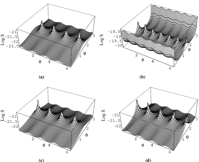
FIG. 4.: Plots of $\log\ S$ of the generators $X^{(A)},A=1,2,3,4$, are displayed in (a), (b), (c) and (d), respectively, as function of $\theta$ and $\phi$ for $f=1$ mHz and SNR = 5.

C Maximisation

In this subsection our goal is to maximise the SNR for a given monochromatic source over the set of noise cancelling combinations. These combinations can be generated by the generators given in the eq. (34) and (39). The SNR corresponding to the each of the generators ($X^{(A)},\ A=1\ {\rm to\ }4$) as a function of frequency are shown in the figure. However one must maximise the SNR over an arbitrary linear combination of $X^{(A)}$. This goal is difficult to achieve since it involves a maximisation over a space of six tuples of polynomials which is essentially a function space. In order to make the problem tractable and still achieve adequate results we restrict the polynomials to be constants. This approach does not fully optimise the SNR but it comes quite close to the optimal solution. Our approach can be thought of as a zero’th order approximation.

A linear combination of the generators can be written as

$$X\ =\ \sum_{A=1}^{4}\alpha_{(A)}X^{(A)},$$ (112)

here, $\alpha_{(A)}$ (for $A$= 1 to 4) are a set of real numbers. Since a scalar multiple of $X$ will not yield anything new, we set one of the $\alpha$’s, say, $\alpha_{(1)}=1$. Thus the SNR now becomes a function of three parameters $\alpha_{(i)},i=2,3,4$, which are just real numbers and our objective is to maximise the SNR with respect to $\alpha_{(i)}$.

In order to carry out the analysis efficiently and elegantly we find that it is useful to define complex noise vectors $N^{(A)}$ pertaining to $X^{(A)}$ as follows:

$$N^{(A)}\ =\ \left(\sqrt{S_{1}}(2p^{(A)}_{i}+r^{(A)}_{i}),\sqrt{S_{1}}(2q^{(A)}_{i}+r^{(A)}_{i}),\sqrt{S_{2}}p^{(A)}_{i},\sqrt{S_{2}}q^{(A)}_{i}\right)$$ (113)

where, $p^{(A)}_{i}$, $q^{(A)}_{i}$ and $r^{(A)}_{i}$ corresponding to generators $X^{(A)}$ are given in the eq. (34) and (60) and $S_{1}\ =\ S^{proofmass}$ and $S_{2}\ =\ S^{shotnoise}$. We have $N^{(A)}~{}~{}\in~{}~{}C^{12}$ the 12 dimensional complex space and the usual scalar product $C^{12}$ induces a norm; $N^{(A)}\cdot{N^{(A)}}^{*}\equiv||N^{(A)}||^{2}$ gives the noise psds corresponding to the basis $X^{(A)}$.

In a similar fashion one can also write the signal corresponding to a particular basis element. We first define the polynomial 6-tuple for each generator $X^{(A)}$ as follows:

$$P^{(A)}\ =\ \left(p^{(A)}_{i},q^{(A)}_{i}\right)\,,$$ (114)

and the GW signal 6-tuple as,

$$H^{*}=\left(F_{V_{i};+}h_{+}+F_{V_{i};\times}h_{\times},\ F_{U_{i};+}h_{+}+F_{U_{i};\times}h_{\times}\right).$$ (115)

The signal for a specific generator $X^{(A)}$ is then written as,

$$h^{(A)}=P^{(A)}.H^{*}$$ (116)

and the corresponding SNR is given by,

$$SNR^{(A)}\ =\ \frac{|h^{(A)}|}{||N^{(A)}||}\ =\ \sqrt{\frac{(P^{(A)}\cdot H^{*})(P^{(A)}\cdot H^{*})^{*}}{N^{(A)}\cdot{N^{(A)}}^{*}}}\,.$$ (117)

For an arbitrary linear combination X (eq. (112)) the noise vector and the signal vector can be expressed as

$$N=\alpha_{(A)}N^{(A)},~{}~{}~{}~{}~{}~{}P=\alpha_{(A)}P^{(A)}\,,$$ (118)

where summation convention has been used. The signal is just the scalar product $h=P.H^{*}=\alpha_{(A)}h^{(A)}$. We omit subscripts $X$ on these quantities.

In this notation the SNR of the combination (112) can be written as,

$$SNR\ =\ \frac{|h|}{||N||}.$$ (119)

Writing out explicitly the sums in the scalar products,

$$(SNR)^{2}\ =\ \frac{\alpha_{(A)}\alpha_{(B)}h^{(A)}{h^{(B)}}^{*}}{\alpha_{(A)}\alpha_{(B)}N^{(A)}\cdot{N^{(B)}}^{*}}\,.$$ (120)

Maximisation with respect to $\alpha_{(2)},\alpha_{(3)},\alpha_{(4)}$ leads to the following three conditions which must be obeyed by $\alpha_{(i)}$ in order to yield the maximum SNR for $X$:

$${\Re(h{h^{(i)}}^{*})\over|h|^{2}}={\Re(N{N^{(i)}}^{*})\over||N||^{2}},$$ (121)

where $\Re(x)$ denotes the real part of the quantity $x$.

To demonstrate the usefulness of the formalism, we consider just two generators $X^{(1)}$ and $X^{(2)}$. We take the $\alpha_{(1)}=1,\alpha_{(2)}=\alpha$ and other two $\alpha$ s zero. Then,

$$X\ =\ X^{(1)}+\alpha X^{(2)}\,.$$ (122)

The eq. (120) reduces to the form,

$${\cal S}\ =\ \frac{a_{1}+2b_{1}\alpha+c_{1}\alpha^{2}}{a_{2}+2b_{2}\alpha+c_{2}\alpha^{2}}\,,$$ (123)

where,

$$a_{1}=|h^{1}|^{2},~{}~{}b_{1}=\Re(h^{1}h^{2*}),~{}~{}c_{1}=|h^{2}|^{2}\,,$$ (124)

$$a_{2}=|N^{1}|^{2},~{}~{}b_{2}=\Re(N^{1}N^{2*}),~{}~{}c_{2}=|N^{2}|^{2}\,.$$ (125)

The condition for the optimisation (121) simplifies to

$$(b_{1}a_{2}-a_{1}b_{2})+(c_{1}a_{2}-a_{1}c_{2})\alpha+(c_{1}b_{2}-b_{1}c_{2})\alpha^{2}\ =\ 0\,.$$ (126)

The two roots of the eq. (126) can be obtained. Here, $\alpha$ is a function of the parameters $f$, $\theta$, $\phi$, $\epsilon$ and $\psi$. One of the solutions of the eq. (126) correspond to the maximum and other correspond to the minimum of the SNR. In a similar fashion one can maximise the SNR by taking any two of the four generators given in the eq. (34) and by taking appropriate $\alpha_{(i)}$ in the eq. (112). We have seen in several cases that maximising over just two generators yields remarkably good results.

FIG. 5.: (a). Log Log plot of the sensitivity $S$ for the generators $X^{(A)}$ as function of $f$ for $\theta=0$, $\phi=0$ over one year observation period for SNR = 5. The curve [X1,X2,X3,X4] depicts the sensitivity of the linear combination of four generators $X^{(A)}$, which gives maximum SNR.

FIG. 5(b). Plot of coefficients $\alpha_{(A)}$ which gives the maximum SNR for linear combinations of all the four $X^{(A)}$ as function of $f$ for $\theta=0$ and $\phi=0$.

FIG. 6.: (a). Log Log plot of the sensitivity $S$ for the generators $X^{(A)}$ as function of $f$ for $\theta=\pi/4$, $\phi=\pi/4$ over one year observation period for SNR = 5. The curve [X1,X2,X3,X4] depicts the sensitivity of the linear combination of four generators $X^{(A)}$ which gives maximum SNR.

FIG. 6(b). Plot of coefficients $\alpha_{(A)}$ which gives the maximum SNR for linear combinations of all the four $X^{(A)}$ as function of $f$ for $\theta=\pi/4$ and $\phi=\pi/4$.

This simple case demonstrates that one can use the solutions given in the eq. (34) to get a better SNR. However, to get full advantage one needs to maximise the SNR over the three $\alpha$’s. In order to optimise the SNR given by the general combination we resort to numerical methods since there is no straight forward method for solving the coupled algebraic equations given by (121). We use the Powell’s method as given in [6] for maximising the SNR over the parameters $\alpha_{(A)}$. The sensitivity $S$ for the generators $X^{(A)}$ and for the maximal SNR combination of $X^{(A)}$’s denoted by [X1,X2,X3,X4] as a function of frequency $f$ has been plotted in figures 5(a) and 6(a). The coresponding values of $\alpha_{(A)}$ are shown in figures 5(b) and 6(b).

VI Concluding Remarks

We have presented in this paper a rigorous and systematic procedure for obtaining data combinations which cancel the laser frequency noise based on algebraic geometrical techniques and commutative algebra. The data combinations cancelling the laser noise have the structure of a module called the module of syzygies. The module is over a ring of polynomials in three variables, corresponding to the three time delays along the three arms of the interferometer. Our formalism can be extended in a straightforward way to include (cancel) the Doppler shifts due to the motion of the optical benches. This module provides us with a choice of data combinations which are in turn linear combinations of the generators of the module. We use this parametrisation to maximise the SNR over frequency for one class of GW sources, namely, those that are monochromatic. We observe that in the plot of sensitivity verses direction angles for the generators $X^{(A)}$, namely figures 4 (a)-(d), the sensitivity has several peaks. It may be possible to employ this property to optimally resolve binaries in the confusion noise regime by considering suitable data combinations which would be sensitive to specific directions in the sky. Also here we have investigated monochromatic GW sources. We believe that this formalism may also be applied successfully to other type of GW sources eg. stochastic GW background.

VII Acknowledgments

The authors thank IFCPAR (project no. 2204 - 1) under which this work has been carried out. The authors are highly indebted to Himanee Arjunwadkar for pains takingly explaining the intricacies of the algebraic geometrical ideas required in this work and also for spending time and effort for the same. SVD would like to thank A. Vecchio, S. Phinney, M. Tinto and T. Prince for fruitful discussions.

A generators of the module of syzygies

We require the 4-tuple solutions $(p_{3},q_{1},q_{2},q_{3})$ to the equation:

$$(xyz-1)p_{3}+(xz-y)q_{1}+x(1-z^{2})q_{2}+(1-x^{2})q_{3}=0\,,$$ (A1)

where for convenience we have substituted $x=E_{1},y=E_{2},z=E_{3}$. $p_{3},q_{1},q_{2},q_{3}$ are polynomials in $x,y,z$ with integral coefficients i.e. in Z[x,y,z].

We now follow the procedure in book by Becker et al. [4].

Consider the ideal in $Z[x,y,z]$ (or $Q[x,y,z]$ where $Q$ denotes the field of rational numbers), formed by taking linear combinations of the coefficients in eq.(A1) $f_{1}=xyz-1,f_{2}=xz-y,f_{3}=x(1-z^{2}),f_{4}=1-x^{2}$. A Groebner basis for this ideal is:

$${\cal G}=\{g_{1}=z^{2}-1,g_{2}=y^{2}-1,g_{3}=x-yz\}\,.$$ (A2)

The above Groebner basis is obtained using the function GroebnerBasis in Mathematica. One can check that both the $f_{i},i=1,2,3,4$ and $g_{j},j=1,2,3$ generate the same ideal because we can express one generating set in terms of the other and vice-versa:

$$f_{i}=d_{ij}g_{j},~{}~{}~{}~{}~{}~{}~{}~{}g_{j}=c_{ji}f_{i}\,,$$ (A3)

where $d$ and $c$ are $4\times 3$ and $3\times 4$ polynomial matrices respectively, and are given by,

$$d=\left(\begin{array}[]{ccc}1&z^{2}&yz\\ y&0&z\\ -x&0&0\\ -1&-z^{2}&-(x+yz)\end{array}\right)\,,\hskip 21.68121ptc=\left(\begin{array}[]{cccc}0&0&-x&z^{2}-1\\ 1&-y&0&0\\ 0&z&1&0\end{array}\right)\,.$$ (A4)

The generators of the 4-tuple module are given by the set $A\,\bigcup B^{*}$ where $A$ and $B^{*}$ are the sets described below:

$A$ is the set of row vectors of the matrix $I-d.c$ where the dot denotes the matrix product and I is the identity matrix, $4\times 4$ in our case. Thus,

$$a_{1} = (1-z^{2},0,x-yz,1-z^{2})\,,$$ (A5)

$$a_{2} = (0,z(1-z^{2}),xy-z,y(1-z^{2}))\,,$$ (A6)

$$a_{3} = (0,0,1-x^{2},x(z^{2}-1))\,,$$ (A7)

$$a_{4} = (z^{2},xz,yz,z^{2})\,.$$ (A8)

We thus first get 4 generators. The additional generators are obtained by computing the S-polynomials of the Groebner basis ${\cal G}$. The S-polynomial of two polynomials $g_{1},g_{2}$ is obtained by multiplying $g_{1}$ and $g_{2}$ by suitable terms and then adding, so that the highest terms cancel. For example in our case $g_{1}=z^{2}-1$ and $g_{2}=y^{2}-1$ and the highest terms are $z^{2}$ for $g_{1}$ and $y^{2}$ for $g_{2}$ . Multiply $g_{1}$ by $y^{2}$ and $g_{2}$ by $z^{2}$ and subtract. Thus, the S-polynomial $p_{12}$ of $g_{1}$ and $g_{2}$ is:

$$p_{12}=y^{2}g_{1}-z^{2}g_{2}=z^{2}-y^{2}\,.$$ (A9)

Note that order is defined ($x>>y>>z$) and the $y^{2}z^{2}$ term cancels. For the Groebner basis of 3 elements we get 3 S-polynomials $p_{12},p_{13},p_{23}$. The $p_{ij}$ must now be rexpressed in terms of the Groebner basis ${\cal G}$. This gives a $3\times 3$ matrix $b$. The final step is to transform to 4-tuples by multiplying $b$ by the matrix $c$ to obtain $b^{*}=b.c$. The row vectors $b^{*}_{i},i=1,2,3$ of $b^{*}$ form the set $B^{*}$:

$$b^{*}_{1} = (1-z^{2},y(z^{2}-1),x(1-y^{2}),(y^{2}-1)(z^{2}-1))\,,$$ (A10)

$$b^{*}_{2} = (0,z(1-z^{2}),1-z^{2}-x(x-yz),(x-yz)(z^{2}-1))\,,$$ (A11)

$$b^{*}_{3} = (x-yz,z-xy,1-y^{2},0).$$ (A12)

Thus we obtain 3 more generators which gives us a total of 7 generators of the required module of syzygies.

B matrices of conversion between generating sets

In this appendix we list the three sets of generators and relations among them. We first list below $\alpha,\beta,\gamma,\zeta$:

$$\alpha = (1,z,xz,1,xy,y)\,,$$ (B1)

$$\beta = (xy,1,x,z,1,yz)\,,$$ (B2)

$$\gamma = (y,yz,1,xz,x,1)\,,$$ (B3)

$$\zeta = (x,y,z,x,y,z)\,.$$ (B4)

We now express the $a_{i}$ and $b^{*}_{j}$ in terms of $\alpha,\beta,\gamma,\zeta$:

$$a_{1} = \gamma-z\zeta\,,$$ (B5)

$$a_{2} = \alpha-z\beta\,,$$ (B6)

$$a_{3} = -z\alpha+\beta-x\gamma+xz\zeta\,,$$ (B7)

$$a_{4} = z\zeta$$ (B8)

$$b^{*}_{1} = -y\alpha+yz\beta+\gamma-z\zeta\,,$$ (B9)

$$b^{*}_{2} = (1-z^{2})\beta-x\gamma+xz\zeta\,,$$ (B10)

$$b^{*}_{3} = \beta-y\zeta\,.$$ (B11)

Further we also list below $\alpha,\beta,\gamma,\zeta$ in terms of $X^{(A)}$:

$$\alpha = X^{(3)}\,,$$ (B12)

$$\beta = X^{(4)}\,,$$ (B13)

$$\gamma = -X^{(1)}+zX^{(2)}\,,$$ (B14)

$$\zeta = X^{(2)}\,.$$ (B15)

This proves that since the $a_{i},b^{*}_{j}$ generate the required module, the $\alpha,\beta,\gamma,\zeta$ and $X^{(A)},A=1,2,3,4$ also generate the same module.

The Groebner basis is given in terms of the above generators as follows: $G^{(1)}=\zeta,G^{(2)}=X^{(1)},G^{(3)}=\beta,G^{(4)}=\alpha$ and $G^{(5)}=a_{3}$.

REFERENCES

- [1] J.W. Armstrong, F. B. Eastabrook and M. Tinto, Ap. J. 527, 814 (1999).
- [2] F.B. Estabrook, M. Tinto and J.W. Armstrong, Phys. Rev, D 62, 042002(2000).
- [3] M. Tinto and J.W. Armstrong, Phys. Rev, D 59, 102003(1999).
- [4] T. Becker, ”Groebner Bases: A computational approach to commutative algebra”, Volker Weispfenning in cooperation with Heinz Kredel, Graduate texts in Mathematics 141, Springer Verlag (1993).
- [5] M. Kreuzer and L. Robbiano, ”Computational commutative algebra 1”, Springer Verlag(2000).
- [6] W.H. Press, S.A. Teukolsky, W.T. Vetterling and B.P. Flannery, ” numerical recipes in C, The art of scientific computing, Sec. ed., Cambridge University press(1999).
- [7] Macaulay2 software by D.R. Grayson and M.E. Stillman, http://www.math.uiuc.edu/Macaulay2/.
- [8] P.L. Bender and D. Hils, CQG, 14, 1439(1997).
- [9] K.A. Postnov and M.E. Prokhorov, Ap.J, 494, 674(1998).
- [10] D.I. Kosenko and K.A. Postnov, A&A, 336, 786(1998).
- [11] D. Hils and P.L. Bender, Ap.J, 537, 334(2000).
- [12] V.B. Ignatiev, A.G Kuranov, K.A Postnov and M.E Prokhorov, MNRAS, 327, 531(2001).
- [13] F. Verbunt and G. Nelemans, CQG, 18, 4005(2001).
- [14] R Schneider, et. al, MNRAS, 324, 797(2001).
- [15] G Nelemans, L.R. Yungelson and S.F. Portegies Zwart, A&A, 375, 890(2001).
- [16] W.A Hiscock, Ap. J., 509, L101(1998).
- [17] K. Ioka, T. Tanaka, T Nakamura, Phys. Rev. D 60, 083512(1999).
- [18] W.A. Hiscock, et. al, Ap. J, 540, L5(2000).
- [19] M. Tinto, J.W. Armstrong and F.B Estabrook, Phys. Rev D 63, 021101(2000).
- [20] R. Schilling, CQG, 14, 1513(1997).
- [21] C. Cutler, Phys. Rev, D 57, 7089(1998).
- [22] ”LISA: A Cornerstone Mission for the Observation of Gravitational Waves”, System and Technology Study Report, 2000.