Classical Radiation Formula in the Rindler Frame

Abstract

In a preceding paper $[$T. Hirayama, Prog. Theor. Phys. 106 (2001), 71$]$, the power of the classical radiation emitted by a moving charge was evaluated in the Rindler frame. In this paper, we give a simpler derivation of this radiation formula, including an estimation of the directional dependence of the radiation. We find that the splitting of the energy-momentum tensor into a bound part $\widetilde{\rm I}$ and an emitted part $\widetilde{\rm II}$ is consistent with the three conditions introduced in the preceding paper, also for each direction within the future light cone.

1 Introduction

In a preceding paper,[1] we calculated the power of the classical elecromagnetic radiation emanated from a moving point charge in the Rindler frame, which is a linearly and uniformly accelerated frame in Minkowski spacetime and also interpreted as a rest frame with a static homogeneous gravitational field.[2] The power was evaluated in terms of the energy defined by the Killing vector field that generates the time of that frame. We found that the power is proportional to the square of the acceleration $\alpha^{\mu}$ of the charge relative to the Rindler frame $[$see Ref. Hi01 or §2 of this paper for the definition of $\alpha^{\mu}]$. This result was interpreted as providing a picture in which the concept of radiation depends on the reference frames or motion of observers,[3] and we discussed it in relation to the old paradox concerning the classical radiation emitted from a uniformly accelerated charge.[5, 6]

In the conventional treatments, radiation is identified with reference to the region sufficiently distant from the charge. (In the case of the Rindler spacetime, this region would correspond to the future horizon.) Actually, the well-known Larmor formula and the above mentioned radiation formula in the Rindler frame are obtained by integrating the energy in that region. However, Rohrlich and Teitelboim proposed another approach,[7, 8, 9] in which the radiation can be identified at an arbitrary distance from the charge, without reference to the asymptotic zone. This provides a picture of radiation as an emission of something by a charge, which begins to exist immediately after emission. This approach consists of splitting the energy-momentum tensor of the retarded field into an emitted part ${\rm II}$ and a bound part ${\rm I}$, which can be done in a natural way using the usual splitting of the retarded field into the acceleration part and the velocity part.[8, 9]

Similarly, we found in Ref. Hi01 that a natural splitting of the energy-momentum tensor into an emitted part $\widetilde{\rm II}$ and a bound part $\widetilde{\rm I}$ exists in the Rindler frame. This splitting was realized by splitting the retarded field into a part linear in $\alpha^{\mu}$ and a part independent of $\alpha^{\mu}$. The emitted nature and bound nature of these parts were confirmed in the sense that they satisfy the following three conditions:[1]

1. A charge fixed in the Rindler frame does not radiate.

2. The emitted part propagates along the future light cone with an apex on the world line of the charge, in the sense that the energy of this part does not damp along the light cone.

3. The bound part does not contribute to the energy in the region $\eta\rightarrow\infty$, where $\eta$ is the time coordinate in the Rindler frame and the limit is taken along the future light cone with an apex on the world line of the charge.
   

The main purpose of this paper is to present a simpler derivation of the radiation formula in the Rindler frame by using retarded coordinates,[9, 10] which are often used to simplify the calculation of retarded quantities around a charge. Simplification also results from the relation expressed in Eq. (9), in which we can characterize the distance between the charge and the future horizon in terms of the null vector $w^{\mu}$, the vector which played a key role in Ref. Hi01. In this calculation, the angular dependence of the radiation is also represented obviously in the integrand of the equation.

In Ref. Hi01, the consistency of splitting the tensor into $\widetilde{\rm I}$ and $\widetilde{\rm II}$ with three conditions was confirmed only after integration over the angular dependence. In this paper, we confirm this consistency for each solid angle element. This procedure is again simplified with the aid of Eq. (9). In these calculations, we use the solid angle defined in the inertial frame. This is reasonable because the limit in which the radiation is identified should be taken along the light ray (null geodesic) that emanates from the charge, and the angular coordinates in the inertial frame are constant along this light ray. It is also pointed out that the radiative energy per solid angle is nonnegative, as would be expected in natural identification of radiation.

Throughout this paper, we use Gaussian units and the metric with signature $(-,+,+,+)$.

2 Simple derivation of the radiation formula

In this section, we calculate the power of the radiation in the Rindler frame by using retarded coordinates, which are defined as follows.[9, 10] For a point $p$ (with coordinates $x^{\mu}$), the retarded point $\bar{p}$ (with coordinates $\bar{x}^{\mu}$) is defined as a point on the worldline of a point charge that satisfies the condition

$$r^{\mu} = x^{\mu}-\bar{x}^{\mu},$$ (1)

$$r^{\mu}r_{\mu} = 0,\ \ \ \ x^{t}>\bar{x}^{t},$$ (2)

expressed in an inertial frame $(t,x,y,z)$. We define the retarded time $\tau$ of a point $p$ as the proper time of a charge at the retarded point $\bar{p}$. The retarded distance $\rho$ is defined as $\rho=-v\cdot r$, where $v$ denotes the 4-velocity of the charge at the point $\bar{p}$. Then we can specify an arbitrary point in the spacetime by the coordinates $\tau$ and $\rho$ and the angular coordinates $\theta$ and $\varphi$ defined in an inertial frame.

We now introduce a ray vector $k^{\mu}=r^{\mu}/\rho$, which has the properties $k\cdot k=0$ and $k\cdot v=-1$. This vector does not depend on $\rho$, and it is expressed as $k^{\mu}=k^{\mu}(\tau,\theta,\varphi)$. The volume element $d\Sigma_{\mu}$ of the 3-dimensional plane $\Sigma$ orthogonal to the vector $N^{\mu}$ is calculated in Appendix A, and the result is

$$d\Sigma^{\mu} = -\frac{N^{\mu}}{N\cdot k}\rho^{2}d\tau d\Omega_{0},$$ (3)

where $d\Omega_{0}$ is the solid angle element of the inertial frame with time axis $v^{\mu}$ $[$see Eq. (40)$]$.

For the inertial coordinates $(t,x,y,z)$, the Rindler coordinates $(\eta,x,y,\xi)$ are given by $t=\xi\sinh\eta$ and $z=\xi\cosh\eta$, with the metric $ds^{2}=-\xi^{2}d\eta^{2}+dx^{2}+dy^{2}+d\xi^{2}$. We can define the energy in the Rindler frame with respect to the time-like Killing vector field $X^{\mu}$ which is proportional to the field

$$\frac{\partial}{\partial\eta} = z\frac{\partial}{\partial t}+t\frac{\partial}{\partial z}.$$ (4)

The Rindler energy over the region $\Sigma$ is given by

$$E_{[X,\Sigma]} = -\int_{\Sigma}d\Sigma_{\mu}X_{\nu}T^{\mu\nu},$$ (5)

where $T^{\mu\nu}$ is the energy-momentum tensor of the electromagnetic field. For free fields, conservation of this quantity is confirmed by the Killing equation $\nabla_{\mu}X_{\nu}+\nabla_{\nu}X_{\mu}=0$ and Gauss’s theorem $[$see §2.1 of Ref. Hi01$]$.

We consider two closely positioned points $\bar{p}$ and $\bar{p}^{\prime}$ on the worldline of the charge (see Fig. 1). Let $\Delta L$ be a region that is bounded on two future light cones with apexes $\bar{p}$ and $\bar{p}^{\prime}$. Let $\sigma(\eta)$ be the intersection of $\Delta L$ with a surface of simultaneity $\eta=[{\rm constant}]$. In the following, we determine the radiation emitted by a moving charge in the Rindler frame by evaluating the Rindler energy of the retarded field in the region $\sigma(\eta\rightarrow\infty)$.

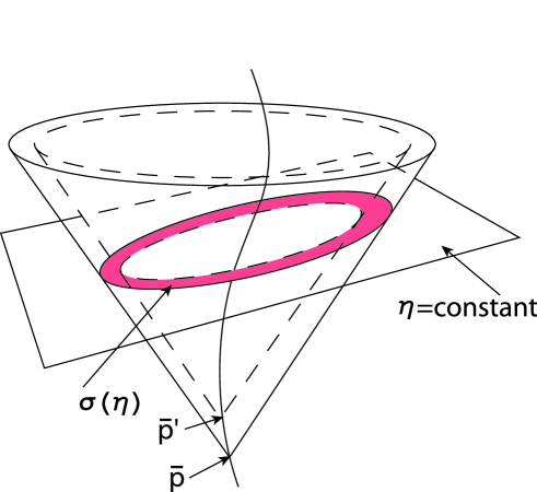
Figure 1: The radiation in the Rindler frame is evaluated with respect to the energy in the region $\lim_{\eta\rightarrow\infty}\sigma(\eta)$. To identify the emitted and bound parts of the Maxwell tensor properly, we introduce three conditions concerning the behavior of these parts along the future light cone.

We here note the relation

$$X\cdot k=\bar{X}\cdot k,$$ (6)

which is satisfied on the future light cone with the apex $\bar{p}$, where $\bar{X}^{\mu}$ is the value of $X^{\mu}$ evaluated at $\bar{p}$. We can prove this relation for general Killing fields in Minkowski spacetime as follows. We can write $k^{\mu}\nabla_{\mu}k^{\nu}=0$, because $k^{\mu}$ is independent of $\rho$. This equation and the Killing equation $\nabla_{\mu}X_{\nu}=-\nabla_{\nu}X_{\mu}$ lead to $k^{\mu}\nabla_{\mu}(X\cdot k)=0$. Thus $X\cdot k$ is constant along the ray vector that emanates from $\bar{p}$.

The volume element for $\sigma(\eta)$ is obtained from Eq. (3) by using $X^{\mu}$ for $N^{\mu}$. Therefore, from Eqs. (5) and (6), the Rindler energy over the region $\sigma(\eta)$ can be expressed as

$$E_{[X,\sigma(\eta),{\rm ret}]} = d\tau\int_{\sigma(\eta)}d\Omega_{0}\frac{\rho^{2}}{\bar{X}\cdot k}X_{\mu}X_{\nu}{T_{\rm ret}}^{\mu\nu},$$ (7)

where ${T_{\rm ret}}^{\mu\nu}$ is the energy-momentum tensor of the retarded field generated by the charge. Except in the direction of $z$, or the $\xi$ axis, the region $\sigma(\eta\rightarrow\infty)$ arrives at the future horizon $H^{+}$. Therefore, we now derive two formulae giving the values of $\rho$ and $X^{\mu}$ at $H^{+}$, in order to evaluate the value of the integrand in Eq. (7) in that region.

Let us consider a null vector $w^{\mu}=(g\cdot g)^{1/2}u^{\mu}+g^{\mu}$, which plays a key role in defining the bound and emitted parts of the Maxwell tensor in Ref. Hi01. Here $u^{\mu}=|X\cdot X|^{-1/2}X^{\mu}|_{\bar{p}}$ and $g^{\mu}=|X\cdot X|^{-1}X^{\nu}\nabla_{\nu}X^{\mu}|_{\bar{p}}$ represent the 4-velocity and the 4-acceleration of the Rindler observer at the point $\bar{p}$, respectively. We here note that throughout this paper, $w^{\mu}$ is considered at the point $\bar{p}$. In the inertial frame $(t,x,y,z)$, $w^{\mu}$ is written

$$(w^{t},w^{x},w^{y},w^{z}) = \frac{1}{\bar{z}-\bar{t}}(1,0,0,1).$$ (8)

The contraction of this quantity with the vector $r^{\mu}|_{H^{+}}$ gives

$$r^{\mu}|_{{}_{H^{+}}}w_{\mu} = -1,$$ (9)

which is obtained by substituting $z=t$, which holds for the future horizon $H^{+}$. To avoid confusion caused by our unfamiliar notation, we here note again that $w^{\mu}$ is evaluated at $\bar{p}$, not at $H^{+}$.

For an inertial frame with time axis $t^{\mu}$, where $t^{\mu}$ is a future-directed vector and $t^{\mu}t_{\mu}=-1$, we introduce the retarded distance $\hat{\rho}=-r^{\mu}t_{\mu}$ and the ray vector $l^{\mu}=r^{\mu}/\hat{\rho}$. Equation (9) divided by the retarded distance $\hat{\rho}|_{H^{+}}$ gives

$$\left.\frac{1}{\ \hat{\rho}\ }\right|_{H^{+}} = -w^{\mu}l_{\mu}.$$ (10)

On the other hand, if a vector $w^{\prime\mu}$ satisfies $\hat{\rho}^{-1}|_{H^{+}}=-w^{\prime\mu}l_{\mu}$, then $w^{\prime\mu}=w^{\mu}$, because we can choose four independent ray vectors $l^{\mu}$ that emanate from $\bar{p}$, and the contractions of these four vectors with $w^{\prime\mu}$ uniquely determine all components of the vector $w^{\prime\mu}$. From this equation, we find that the distance between the observer and the event horizon $H^{+}$ is charactarized by a unique vector $w^{\mu}$, and that this expression is the same for any inertial frame, i.e., independent of the choice of $t^{\mu}$.

For the inertial frame with the time axis $v^{\mu}$, Eq. (10) reduces to

$$\left.\frac{1}{\ \rho\ }\right|_{H^{+}} = -w^{\mu}k_{\mu}.$$ (11)

Using this equation and noting that $X^{\mu}|_{H^{+}}\propto w^{\mu}$, we find that $X^{\mu}/\rho|_{H^{+}}=-(w\cdot k)X^{\mu}|_{H^{+}}=-(X\cdot k)|_{H^{+}}w^{\mu}$. From Eq. (6), we obtain the formula for evaluating $X^{\mu}$ at $H^{+}$,

$$\left.\frac{X^{\mu}}{\rho}\right|_{H^{+}} = -(\bar{X}\cdot k)w^{\mu}.$$ (12)

Now we can evaluate the radiative power in the region $H^{+}$ by using Eqs. (11) and (12) in Eq. (7) in the limit $\eta\rightarrow\infty$, with the explicit form of ${T_{\rm ret}}^{\mu\nu}$ given as $[$see Eq. (A$\cdot$17) in Ref. Hi01 or Eq. (2.7) in Ref. Te70, and also Eq. (24) in this paper.$]$

$${T_{\rm ret}}^{\mu\nu} = {T_{{\rm I},{\rm I}}}^{\mu\nu}+{T_{{\rm I},{\rm II}}}^{\mu\nu}+{T_{{\rm II},{\rm II}}}^{\mu\nu},$$ (13)

$$\frac{4\pi}{e^{2}}{T_{{\rm I},{\rm I}}}^{\mu\nu} = \frac{1}{\rho^{4}}\left[k^{\mu}k^{\nu}-(v^{\mu}k^{\nu}+k^{\mu}v^{\nu})-\frac{1}{2}\eta^{\mu\nu}\right],$$ (14)

$$\frac{4\pi}{e^{2}}{T_{{\rm I},{\rm II}}}^{\mu\nu} = \frac{1}{\rho^{3}}[2(a\cdot k)k^{\mu}k^{\nu}-(a\cdot k)(v^{\mu}k^{\nu}+k^{\mu}v^{\nu})-(a^{\mu}k^{\nu}+k^{\mu}a^{\nu})],$$ (15)

$$\frac{4\pi}{e^{2}}{T_{{\rm II},{\rm II}}}^{\mu\nu} = \frac{1}{\rho^{2}}[(a\cdot k)^{2}-a\cdot a]k^{\mu}k^{\nu},$$ (16)

where $v^{\mu}$ and $a^{\mu}$ are the 4-vector and the 4-acceleration of the charge evaluated at the retarded point $\bar{p}$. First, let us consider the contribution from ${T_{{\rm I},{\rm I}}}^{\mu\nu}$. From Eqs. (12) and (14), we find

$$\left.\frac{\rho^{2}}{\bar{X}\cdot k}\frac{4\pi}{e^{2}}{T_{{\rm I},{\rm I}}}^{\mu\nu}X_{\mu}X_{\nu}\right|_{H^{+}} = \left.\rho^{4}(\bar{X}\cdot k)\frac{4\pi}{e^{2}}{T_{{\rm I},{\rm I}}}^{\mu\nu}w_{\mu}w_{\nu}\right|_{H^{+}}$$ (17)

$$= (\bar{X}\cdot k)w\cdot k(w\cdot k-2v\cdot w)$$

$$= (\bar{X}\cdot k)\left[(w_{\perp}\cdot k)^{2}-(w_{\perp}\cdot w_{\perp})\right].$$

Here ${w_{\perp}}^{\mu}=h^{\mu}_{\ \nu}w^{\nu}$, where $h^{\mu}_{\ \nu}=\delta^{\mu}_{\ \nu}+v^{\mu}v_{\nu}$ is the projector onto the plane orthogonal to $v^{\mu}$. We find, similarly, for ${T_{{\rm I},{\rm II}}}^{\mu\nu}$,

$$\left.\frac{\rho^{2}}{\bar{X}\cdot k}\frac{4\pi}{e^{2}}{T_{{\rm I},{\rm II}}}^{\mu\nu}X_{\mu}X_{\nu}\right|_{H^{+}} = 2(\bar{X}\cdot k)\left[a\cdot w_{\perp}-(a\cdot k)w_{\perp}\cdot k\right]$$ (18)

To determine the contribution from ${T_{{\rm II},{\rm II}}}^{\mu\nu}$, it is not necessary to use the formulae (11) and (12), because this contribution is independent of the distance $\rho$ from the charge, and therefore we do not need to consider quantities in the region $H^{+}$. From Eqs. (16) and (6), we obtain

$$\frac{\rho^{2}}{\bar{X}\cdot k}\frac{4\pi}{e^{2}}{T_{{\rm II},{\rm II}}}^{\mu\nu}X_{\mu}X_{\nu} = (\bar{X}\cdot k)\left[(a\cdot k)^{2}-a\cdot a\right],$$ (19)

for the region $\sigma(\eta)$ with arbitrary $\eta$.

In Eqs. (17) and (18), we have evaluated the integrands in the region $H^{+}$. However, we should also evaluate these quantities in the region $I^{+}$, defined by the limit $\eta\rightarrow\infty$ along the light ray parallel to the $z$ axis. In this case, the limit $\eta\rightarrow\infty$ is equivalent to the limit $\rho\rightarrow\infty$. Estimating the $\rho$ dependence of $\rho^{2}{T_{{\rm I},{\rm I}}}^{\mu\nu}X_{\mu}X_{\nu}$ and $\rho^{2}{T_{{\rm I},{\rm II}}}^{\mu\nu}X_{\mu}X_{\nu}$ in this direction, we find that these quantities disappear in $I^{+}$. On the other hand, the right-hand sides of Eqs. (17) and (18) are equal to zero for $k^{\mu}$ directed forward $I^{+}$, and we thus confirm that these equations can be extended to the region $I^{+}$.

Combining Eqs. (17)–(19), we obtain the angular dependence of the radiated power,

$$\lim_{\eta\rightarrow\infty}E_{[X,\sigma(\eta),{\rm ret}]} = -\lim_{\eta\rightarrow\infty}\int_{\sigma(\eta)}d\Sigma_{\mu}X_{\nu}{T_{\rm ret}}^{\mu\nu}$$ (20)

$$= \frac{e^{2}}{4\pi}d\tau\oint d\Omega_{0}(\bar{X}\cdot k)\left[(\alpha\cdot k)^{2}-\alpha\cdot\alpha\right],$$

where $\alpha^{\mu}=h^{\mu}_{\ \nu}(a^{\nu}-w^{\nu})=a^{\mu}-{w_{\perp}}^{\mu}$. By using the formulae

$$\oint d\Omega_{0}{k_{\perp}}^{\mu}=0,\ \ \ \ \oint d\Omega_{0}{k_{\perp}}^{\mu}{k_{\perp}}^{\nu}{k_{\perp}}^{\lambda}=0,\ \ \ \ \oint d\Omega_{0}{k_{\perp}}^{\mu}{k_{\perp}}^{\nu}=\frac{4\pi}{3}h^{\mu\nu},$$ (21)

where ${k_{\perp}}^{\mu}=h^{\mu}_{\ \nu}k^{\nu}=k^{\mu}-v^{\mu}$, the total radiated energy in the Rindler frame is obtained as

$$\lim_{\eta\rightarrow\infty}E_{[X,\sigma(\eta),{\rm ret}]} = \frac{2e^{2}}{3}\alpha^{\mu}\alpha_{\mu}(-\bar{X}\cdot v)d\tau.$$ (22)

At the instant that the charge is at rest in the Rindler frame (where $v^{\mu}=u^{\mu}$), we have $\alpha^{\mu}=a^{\mu}-g^{\mu}$. Therefore $\alpha^{\mu}$ should be interpreted as the acceleration of the charge relative to the Rindler frame.[1] We find from Eq. (22) that radiation is generated in the Rindler frame if and only if the charge deviates from the trajectory  $\alpha^{\mu}=0$.

3 Bound and emitted parts of the Maxwell tensor

We have treated the situation in which the electromagnetic field surrounding the moving charge is expressed by the retarded field, which is given as $[$see Eq. (2.3) in Ref. Te70$]$

$${F_{\rm ret}}^{\mu\nu} = {F_{\ {\rm I}}}^{\mu\nu}+{F_{\ {\rm II}}}^{\mu\nu},$$

$${F_{\ {\rm I}}}^{\mu\nu} = \frac{e}{\rho^{2}}(v^{\mu}k^{\nu}-k^{\mu}v^{\nu}),$$

$${F_{\ {\rm II}}}^{\mu\nu} = \frac{e}{\rho}a\cdot k(v^{\mu}k^{\nu}-k^{\mu}v^{\nu})+\frac{e}{\rho}(a^{\mu}k^{\nu}-k^{\mu}a^{\nu}),$$ (23)

where ${F_{\ {\rm I}}}^{\mu\nu}$ and ${F_{\ {\rm II}}}^{\mu\nu}$ behave as $\sim\rho^{-2}$ and $\sim\rho^{-1}$, respectively. In conventional treatments in inertial frames, the former part is interpreted as being bound to the charge, and the latter as being emitted from the charge. By using this splitting, Teitelboim split the energy momentum tensor into the form (see Eqs. (14)–(16))

$${T_{\rm ret}}^{\mu\nu} = {T_{\ {\rm I}}}^{\mu\nu}+{T_{\ {\rm II}}}^{\mu\nu},$$

$${T_{\ {\rm I}}}^{\mu\nu} = {T_{\ {\rm I},{\rm I}}}^{\mu\nu}+{T_{\ {\rm I},{\rm II}}}^{\mu\nu},\ \ \ {T_{\ {\rm II}}}^{\mu\nu}={T_{\ {\rm II},{\rm II}}}^{\mu\nu},$$ (24)

where the emitted part ${T_{\ {\rm II}}}^{\mu\nu}$ is composed of the field ${F_{\ {\rm II}}}^{\mu\nu}$, while the bound part ${T_{\ {\rm I}}}^{\mu\nu}$ includes the pure ${F_{\ {\rm I}}}^{\mu\nu}$ part (denoted by ${T_{\ {\rm I},{\rm I}}}^{\mu\nu}$) and the interference between ${F_{\ {\rm I}}}^{\mu\nu}$ and ${F_{\ {\rm II}}}^{\mu\nu}$ (denoted by ${T_{\ {\rm I},{\rm II}}}^{\mu\nu}$).[8]

We now note that the radiation formula given in Eq. (22) resembles the Larmor formula, where the $a^{\mu}$ dependence in the latter is replaced by $\alpha^{\mu}$ dependence in the former. In analogy to the $a^{\mu}$ dependence found in the splitting (23), we introduced the following splitting of the field for the Rindler frame $[$see Eq. (2$\cdot$36) in Ref. Hi01$]$:

$${F_{\rm ret}}^{\mu\nu} = {F_{\ \widetilde{\rm I}}}^{\mu\nu}+{F_{\ \widetilde{\rm II}}}^{\mu\nu},$$

$${F_{\ \widetilde{\rm I}}}^{\mu\nu} = \frac{e}{\rho^{2}}(v^{\mu}k^{\nu}-k^{\mu}v^{\nu})+\frac{e}{\rho}{w_{\perp}}\cdot k(v^{\mu}k^{\nu}-k^{\mu}v^{\nu})+\frac{e}{\rho}({w_{\perp}}^{\mu}k^{\nu}-k^{\mu}{w_{\perp}}^{\nu}),$$

$${F_{\ \widetilde{\rm II}}}^{\mu\nu} = \frac{e}{\rho}\alpha\cdot k(v^{\mu}k^{\nu}-k^{\mu}v^{\nu})+\frac{e}{\rho}(\alpha^{\mu}k^{\nu}-k^{\mu}\alpha^{\nu}).$$ (25)

Here, the first part is independent of $\alpha^{\mu}$, while the second part is linear in $\alpha^{\mu}$. This splitting inplies the following splitting of the energy-momentum tensor into the emitted part ${T_{\ \widetilde{\rm II}}}^{\mu\nu}$ and the bound part ${T_{\ \widetilde{\rm I}}}^{\mu\nu}$ $[$Eq. (2$\cdot$37) in Ref. Hi01$]$:

$${T_{\rm ret}}^{\mu\nu} = {T_{\ \widetilde{\rm I}}}^{\mu\nu}+{T_{\ \widetilde{\rm II}}}^{\mu\nu},$$

$${T_{\ \widetilde{\rm I}}}^{\mu\nu} = {T_{\ \widetilde{\rm I},\widetilde{\rm I}}}^{\mu\nu}+{T_{\ \widetilde{\rm I},\widetilde{\rm II}}}^{\mu\nu}.$$ (26)

Here, the emitted part ${T_{\ \widetilde{\rm II}}}^{\mu\nu}$ is composed of the field ${F_{\ \widetilde{\rm II}}}^{\mu\nu}$, while the bound part ${T_{\ \widetilde{\rm I}}}^{\mu\nu}$ includes the pure ${F_{\ \widetilde{\rm I}}}^{\mu\nu}$ part (denoted by ${T_{\ \widetilde{\rm I},\widetilde{\rm I}}}^{\mu\nu}$) and the interference between ${F_{\ \widetilde{\rm I}}}^{\mu\nu}$ and ${F_{\ \widetilde{\rm II}}}^{\mu\nu}$ (denoted by ${T_{\ \widetilde{\rm I},\widetilde{\rm II}}}^{\mu\nu}$). The explicit forms of these parts are

$$\frac{4\pi}{e^{2}}{T_{\ \widetilde{\rm I},\widetilde{\rm I}}}^{\mu\nu} = \frac{1}{\rho^{6}}[1+(w\cdot r)^{2}+2(w\cdot r)-2\rho(w\cdot r)(v\cdot w)-2\rho(v\cdot w)]r^{\mu}r^{\nu}$$ (27)

$$-\frac{1}{\rho^{5}}(1+w\cdot r)[v^{\mu}r^{\nu}+r^{\mu}v^{\nu}]-\frac{1}{\rho^{4}}[w^{\mu}r^{\nu}+r^{\mu}w^{\nu}]-\frac{1}{2\rho^{4}}g^{\mu\nu},$$

$$\frac{4\pi}{e^{2}}{T_{\ \widetilde{\rm I},\widetilde{\rm II}}}^{\mu\nu} = \frac{2}{\rho^{6}}[(\alpha\cdot r)\{1+w\cdot r-\rho(v\cdot w)\}-\rho^{2}(w\cdot\alpha)]r^{\mu}r^{\nu}$$ (28)

$$-\frac{1}{\rho^{5}}(\alpha\cdot r)[v^{\mu}r^{\nu}+r^{\mu}v^{\nu}]-\frac{1}{\rho^{4}}[\alpha^{\mu}r^{\nu}+r^{\mu}\alpha^{\nu}],$$

$$\frac{4\pi}{e^{2}}{T_{\ \widetilde{\rm II}}}^{\mu\nu} = \frac{1}{\rho^{6}}[(\alpha\cdot r)^{2}-\rho^{2}(\alpha\cdot\alpha)]r^{\mu}r^{\nu}.$$ (29)

Note that these expressions are independent of, linear in, and quadratic in $\alpha^{\mu}$, respectively. We here note that the emitted and bound parts of the energy-momentum tensor are conserved separately,

$$\nabla_{\mu}{T_{\ \widetilde{\rm I}}}^{\mu\nu}=0,\ \ \ \ \ \nabla_{\mu}{T_{\ \widetilde{\rm II}}}^{\mu\nu}=0,$$ (30)

off the world line of the charge. $[$See Eqs. (2$\cdot$38c) and (2$\cdot$39c) in Ref. Hi01. A simple derivation of these equations is given above Eq. (2$\cdot$26) in that reference.$]$

As mentioned in §1, the validity of identificating these parts as the bound and emitted parts was confirmed by applying the three conditions introduced in Ref. Hi01. However, that was accomplished only after the angular integration of the Rindler energy over $\sigma(\eta)$. In the following, we show that the three conditions hold also for each element of solid angle.

Condition 1 for each direction is confirmed trivially, because the tensor in Eq. (29) itself disappears when $\alpha^{\mu}=0$, which includes the case that the charge is fixed in the Rindler frame. We now consider Condition 2, using analysis similar to that used in the inertial case (see section 4 of Ref. TV80). For a 4-dimensional region $S$ with a boundary $\partial S$, we have a conservation law for the tensor satisfying $\nabla_{\mu}T^{\mu\nu}=0$ within the region $S$,

$$\int_{\partial S}d\Sigma_{\mu}X_{\nu}T^{\mu\nu}=0,$$ (31)

where $d\Sigma_{\mu}$ is the volume element of $\partial S$. This relation can be demonstrated using the Killing equation and Gauss’s theorem $[$see Eq. (2$\cdot$1) in Ref. Hi01$]$. Let us consider the segment $d\Omega_{0}(\eta_{1})$ of $\sigma(\eta_{1})$ and the segment $d\Omega_{0}(\eta_{2})$ of $\sigma(\eta_{2})$ constituting the same solid angle $d\Omega_{0}$. Then, applying the conservation law (31) to the region between $d\Omega_{0}(\eta_{1})$ and $d\Omega_{0}(\eta_{2})$ specified by different times $\eta_{1}\neq\eta_{2}$, and noting $X_{\nu}{T_{\ \widetilde{\rm II}}}^{\mu\nu}\propto k^{\mu}$, we obtain

$$E_{[X,d\Omega_{0}(\eta_{1}),\widetilde{\rm II}]} = E_{[X,d\Omega_{0}(\eta_{2}),\widetilde{\rm II}]}.$$ (32)

This equation shows that Condition 2 holds for each element of solid angle. We can also confirm that the radiative energy in each direction is nonnegative, because $\rho^{2}(\alpha\cdot\alpha)-(\alpha\cdot r)^{2}\geq 0$ in Eq. (29), and therefore the Rindler energy density of the part $\widetilde{\rm II}$ is always nonnegative.

Next, we examine Condition 3 for each direction. Except in the direction of the $z$ axis, this is simplified by using Eq. (9) again. The angular dependence of the Rindler energy is given in Eq. (7). Hence, by noting $X^{\mu}|_{H^{+}}\propto w^{\mu}$, we find that it is sufficient for our purpose to confirm ${T_{\widetilde{\rm I}}}^{\mu\nu}|_{H^{+}}w_{\mu}w_{\nu}=0$. We can confirm this relation by contracting Eqs. (27) and (28) with $w^{\mu}$ and applying Eq. (9). For the direction of the $z$ axis, we find $w^{\mu}r_{\mu}=0$, because of $w^{\mu}\propto r^{\mu}$. We can make the calculation somewhat simpler by using this relation and Eq. (6). Finally, we obtain $\rho^{2}{T_{\widetilde{\rm I},\widetilde{\rm I}}}^{\mu\nu}X_{\mu}X_{\nu}\sim\rho^{-1}$ and $\rho^{2}{T_{\widetilde{\rm I},\widetilde{\rm II}}}^{\mu\nu}X_{\mu}X_{\nu}\sim\rho^{-1}$ in the $z$ direction. Therefore, we find that these contributions disappear in the region $I^{+}$. From these results in $H^{+}$ and $I^{+}$, we find that Condition 3 holds for each element of solid angle.

4 Conclusion

We have obtained a simpler derivation of the radiation formula in the Rindler frame by using retarded coordinates, which are often used to simplify the integration of retarded quantities around a charge. Simplification also results from Eq. (9) or Eq. (11), with which we can characterize the distance between the charge and the future horizon by the vector $w^{\mu}$, the vector which played a key role in the analysis of Ref Hi01. In the retarded coordinates, we can also express the angular dependence of the radiation. Then, we have confirmed that the splitting of the energy-momentum tensor into the bound part $\widetilde{\rm I}$ and emitted part $\widetilde{\rm II}$ satisfies the three conditions (see §1) also in each element of solid angle.

Appendix A Retarded Coordinates

In this appendix, we calculate the volume element of the 3-dimensional plane $\Sigma$ orthogonal to the vector $N^{\mu}$ given in Eq (3). We start with describing the general properties of the retarded coordinates.[9, 10]

The direction of $k^{\mu}$ is invariant when $\tau$ is varied with $\theta$ and $\varphi$ fixed. This invariance is expressed as $\partial k^{\mu}/\partial\tau\propto k^{\mu}$. This property and differentiation of $k\cdot v=-1$ with respect to $\tau$ lead to

$$\frac{\partial k^{\mu}}{\partial\tau} = (k\cdot a)k^{\mu},$$ (33)

where $a^{\mu}=dv^{\mu}/d\tau$ is the 4-acceleration of the charge. Using this, the total derivative of $x^{\mu}=\bar{x}^{\mu}+\rho k^{\mu}$ gives

$$dx^{\mu} = [v^{\mu}+\rho(r\cdot a)k^{\mu}]d\tau+k^{\mu}d\rho+\rho[k_{\theta}^{\mu}d\theta+k_{\varphi}^{\mu}d\varphi],$$ (34)

where $k^{\mu}_{\theta}=\partial k^{\mu}/\partial\theta$ and $k^{\mu}_{\varphi}=\partial k^{\mu}/\partial\varphi$.

From $k\cdot k=0$ and $k\cdot v=-1$, we obtain the orthogonality relations $k_{\theta}\cdot k=k_{\varphi}\cdot k=k_{\theta}\cdot v=k_{\varphi}\cdot v=0$. We can also set $k_{\theta}\cdot k_{\varphi}=0$, since from Eq. (33) we get

$$\frac{\partial}{\partial\tau}(k_{\theta}\cdot k_{\varphi}) = 2(k\cdot a)(k_{\theta}\cdot k_{\varphi}),$$ (35)

so that, if we set $(k_{\theta}\cdot k_{\varphi})=0$ at one time, it holds for all time. Now, we also set $k^{\mu}_{\perp}=h^{\mu}_{\ \nu}k^{\nu}=k^{\mu}-v^{\mu}$, where $h^{\mu}_{\ \nu}=\delta^{\mu}_{\ \nu}+v^{\mu}v_{\nu}$ is the projector onto the plane orthogonal to $v^{\mu}$. We find that $k_{\perp}\cdot k_{\perp}=1$ and that $v^{\mu}$, $k^{\mu}_{\perp}$, $k^{\mu}_{\theta}$ and $k^{\mu}_{\varphi}$ constitute an orthogonal basis.

We now calculate the volume element of the 3-dimensional plane $\Sigma$. For any displacement within the plane, we find $N^{\mu}dx_{\mu}=0$. From this and Eq. (34), we obtain

$$d_{\tau}x^{\mu} = \left(v^{\mu}-\frac{N\cdot v}{N\cdot k}k^{\mu}\right)d\tau,$$

$$d_{\theta}x^{\mu} = \left(k^{\mu}_{\theta}-\frac{N\cdot k_{\theta}}{N\cdot k}k^{\mu}\right)\rho d\theta,$$

$$d_{\varphi}x^{\mu} = \left(k^{\mu}_{\varphi}-\frac{N\cdot k_{\varphi}}{N\cdot k}k^{\mu}\right)\rho d\varphi,$$ (36)

where $d_{\tau}x^{\mu}$ is the displacement within $\Sigma$ when $\tau$ alone varies, and $d_{\theta}x^{\mu}$ and $d_{\varphi}x^{\mu}$ are displacements within $\Sigma$ when $\theta$ and $\varphi$ alone vary, respectively. The volume element $d\Sigma_{\mu}$ of $\Sigma$ is given by

$$d\Sigma_{\mu} = \epsilon_{\mu\nu\lambda\rho}d_{\tau}x^{\nu}d_{\theta}x^{\lambda}d_{\varphi}x^{\rho},$$ (37)

where $\epsilon_{\mu\nu\lambda\rho}$ is the Levi-Civita permutation symbol. From Eq. (36), we have

$$d\Sigma_{\mu} = \rho^{2}d\tau d\theta d\varphi\left(\epsilon_{\mu\nu\lambda\rho}v^{\nu}k^{\lambda}_{\theta}k^{\rho}_{\varphi}-\frac{N\cdot k_{\varphi}}{N\cdot k}\epsilon_{\mu\nu\lambda\rho}v^{\nu}k^{\lambda}_{\theta}k^{\rho}\right.$$ (38)

$$\hskip 65.44142pt\left.-\frac{N\cdot k_{\theta}}{N\cdot k}\epsilon_{\mu\nu\lambda\rho}v^{\nu}k^{\lambda}k^{\rho}_{\varphi}-\frac{N\cdot v}{N\cdot k}\epsilon_{\mu\nu\lambda\rho}k^{\nu}k^{\lambda}_{\theta}k^{\rho}_{\varphi}\right).$$

The first term on the right-hand side of this relation is orthogonal to $v^{\mu}$, $k_{\theta}^{\mu}$ and $k_{\varphi}^{\mu}$, and therefore it is proportional to $k_{\perp}^{\mu}$. Similarly, the second, third and fourth terms are proprtional to $k_{\varphi}^{\mu}$, $k_{\theta}^{\mu}$ and $k^{\mu}$ respectively. Proportionality factors are obtained by contraction with $k_{\perp}^{\mu}$, $k_{\varphi}^{\mu}$, $k_{\theta}^{\mu}$ and $k^{\mu}$. We find

$$d\Sigma^{\mu} = \rho^{2}d\tau d\Omega_{0}\left[-\frac{k_{\perp}^{\mu}}{k_{\perp}\cdot k_{\perp}}-\frac{N\cdot k_{\varphi}}{N\cdot k}\frac{k_{\varphi}^{\mu}}{k_{\varphi}\cdot k_{\varphi}}-\frac{N\cdot k_{\theta}}{N\cdot k}\frac{k_{\theta}^{\mu}}{k_{\theta}\cdot k_{\theta}}+\frac{N\cdot v}{N\cdot k}k^{\mu}\right],$$ (39)

where

$$d\Omega_{0} = \epsilon_{\lambda\mu\nu\rho}v^{\lambda}k^{\mu}k_{\theta}^{\nu}k_{\varphi}^{\rho}d\theta d\varphi$$ (40)

is the solid angle element for the inertial frame with time axis $v^{\mu}$. In Eq. (37), the volume element $d\Sigma^{\mu}$ is assumed to be orthogonal to the plane $\Sigma$. This can be verified by rewriting $N^{\mu}$ in terms of the orthogonal basis $v^{\mu}$, $k^{\mu}_{\perp}$, $k^{\mu}_{\theta}$ and $k^{\mu}_{\varphi}$, and comparing the result with Eq. (39). Finally, we obtain Eq. (3).

References

[1]
T. Hirayama,
Prog. Theor. Phys. 106 (2001), 71, gr-qc/0102082.
[2]
W. Rindler, Am. J. Phys. 34 (1966), 1174.
[3]
This point of view was discussed in analogy with the quantum
theory (Unruh effect)[4] in M. Pauri and M. Vallisneri,
Found. Phys. 29 (1999), 1499, gr-qc/9903052.
[4]
N. D. Birrell and P. C. W. Davies, Quantum Fields in
Curved Space
(Cambridge University Press, Cambridge, 1982).
[5]
T. Fulton and F. Rohrlich,
Ann. of Phys. 9 (1960), 499.
[6]
D. G. Boulware, Ann. of Phys. 124 (1980), 169.
[7]
F. Rohrlich, Nuovo Cim. 21 (1961), 811.
[8]
C. Teitelboim, Phys. Rev. D 1 (1970), 1572.
[9]
C. Teitelboim, D. Villarroel and Ch. G. Van Weert,
Riv. Nuovo Cim. 3, No. 9 (1980).