Hydrodynamics of Galactic Dark Matter

Luis G. Cabral-Rosetti^a , Tonatiuh Matos^b ,

Darío Nuñez^a,c and Roberto A. Sussman^a

^aInstituto de Ciencias Nucleares,
Universidad Nacional Autónoma de México, (ICN-UNAM).
Circuito Exterior, C.U., Apartado Postal 70-543, 94510 México, D.F., México.

^bDepartamento de Física,
Centro de Investigación y de Estudios Avanzadas del IPN,
Apartado Postal 14-740, México D. F., México.

^cCenter for Gravitational Physics and Geometry,
Penn State University,
University Park, PA 16802, U.S.A.

We consider simple hydrodynamical models of galactic dark matter in which the galactic halo is a self-gravitating and self-interacting gas that dominates the dynamics of the galaxy. Modeling this halo as a sphericaly symmetric and static perfect fluid satisfying the field equations of General Relativity, visible barionic matter can be treated as “test particles” in the geometry of this field. We show that the assumption of an empirical “universal rotation curve” that fits a wide variety of galaxies is compatible, under suitable approximations, with state variables characteristic of a non-relativistic Maxwell-Boltzmann gas that becomes an isothermal sphere in the Newtonian limit. Consistency criteria lead to a minimal bound for particle masses in the range $30\,\hbox{eV}\leq m\leq 60\,\hbox{eV}$ and to a constraint between the central temperature and the particles mass. The allowed mass range includes popular supersymmetric particle candidates, such as the neutralino, axino and gravitino, as well as lighter particles ($m\approx$ keV) proposed by numerical N-body simulations associated with self-interactive CDM and WDM structure formation theories.

PACS: 95.35.+d, 95.30.Sf, 98.80.-k

1 Introduction

The presence of large amounts of dark matter at the galactic lengthscale is already an established fact. Assuming that this dark matter is a gas (or gas mixture) of various particles species, the established classification criteria labels possible dark matter forms as “cold” or “hot”, depending on the relativistic or non-relativistic nature of the particles’ energetic spectrum at their decoupling from the cosmic mixture [1], [2], [3]. Hot dark matter (HDM) scenarios seem to be incompatible with current theories of structure formation and thus, are not favoured dark matter candidates [2], [3], [4]. Cold dark matter (CDM), usualy examined within a newtonian framework, can be considered as non-interactive (a self gravitating gas of collisionless particles) or self-interactive [5]. CDM models are often developed in terms of n-body numerical simmulations [6], [7], [8], [9]. Non-interactive CDM models present the following discrepancies with observations at the galactic scale [10], [11]: (a) the “substructure problem” related to excess clustering on sub-galactic scales, (b) the “cusp problem” characterized by a monotonic increase of density towards the center of halos, leading to excessively concentrated cores. These problems appear in the more recent numerical simulations (see [7], [8], [9]). In order to deal with these problems, the possibility of self-interacting dark matter has been considered, so that nonzero pressure or thermal effects can emerge, thus leading to self-interactive models of CDM (i.e. SCDM) [12], [13], [14], [15], [16] and “warm” dark matter (WDM) models [17]-[22] that challenges the duality CDM vs. HDM. Other proposed dark matter sources consist replacing the gas of particles approach by scalar fields [23], [24] and even more “exotic” sources [25].

Whether based on SCDM or WDM, current theories of structure formation point towards dark matter characterized by particles having a mass of the order of at least keV’s (see [12]-[22]), thus suggesting that massive but light particles, such as electron neutrinos and axions (see Table 1), should be eliminated as primary dark matter candidates (though there is no reason to assume that these particles would be absent in galactic halos). Of all possible particle candidates (denoted as WIMP’s: weakly interactive massive particles) complying with the required mass value of relique gases, only the massive neutrinos (the muon or tau neutrinos), have been detected, whereas other WIMPS (gravitino, sterile neutrino, axino, etc.) are speculative. See [26], [27], [28], [29] and Table 1 for a list of candidate particles and appropriate references.

Even if the dynamics of visible matter in galaxies can be described succesfuly with Newtonian gravity, we believe that General Relativity is an appropriate framework for understanding basic features of galactic dark matter, a gravitational field source whose precise physical nature still remains an open question. If the results obtained with GR coincide with Newtonian results, then there is no harm done from a pragmatic calculations-oriented point of view. However, from a formal-theoretical approach, we believe it is beneficial to broaden the scope of the study of galactic dynamics by incorporating it to a more general gravitational theory. In particular, in this paper we aim at testing the compatibility between observed galactic rotation curves and simple thermodynamical assumptions under the framework of GR.

Since dark matter halo probably constitutes the overwhelming mayority (90 %) of the galactic mass, an alternative approach to numerical simulations and newtonian hydrodynamics follows by a general relativistic model describing the gravitational field of the galaxy as a spacetime geometry generated by the the dark matter halo (as a self gravitating gas), hence visible matter becomes test particles that evolve along stable geodesics of this spacetime. There is strong empiric evidence that the radial profile of rotational velocities (“rotation curves”) in most galaxies roughly fits a “universal rotation curve” (URC) [30], [31]. This URC is characterized by a “flattening” effect whereby rotation velocities tend to a constant “terminal” velocity whose value depends on the type of galaxy (between $125\,\hbox{km/sec}$ and $250\,\hbox{km/sec}$). The profile of rotation curves identifies two main contributions of galactic matter: visible matter (the disk), showing a keplerian decay, and dark matter (the halo), explaining the flattening effect. This kinematic evidence might allow us to determine (at least partialy) the geometry of the spacetime associated with a self gravitating galaxy. In other words, our approach somehow inverts the standard initial value procedure in general relativistic hydrodynamics: instead of prescribing initial data based on physicaly motivated sources and then find the geometry of spacetime and the trayectories of test particles after solving Einstein’s equations, we provide first constraints on the geometry of spacetime (from symmetry criteria and empirical kinematic data) and then find, with the help of the field equations, the corresponding momentum-energy tensor of the sources. This approach to galactic dark matter has been used in connection to scalar fields [23].

Bearing in mind that the dark matter halo overwhelmingly dominates the galactic matter content (at least in the halo region), we shall assume that the galactic halo (as a self gravitating gas) is the unique matter source of the galactic spacetime. Visible matter becomes then test observers that follow stable circular geodesic orbits (the galactic rotation curves) of this spacetime. Following the “inverse” approach described above, we propose to use the empiric law governing the form of the URC for the galactic halo (see [30] and [31]) in order to make specific asertions on the nature of the sources of the galactic spacetime. Considering the self-gravitating galactic halo gas to be self-interactive (instead of colissionless matter or a scalar field), we aim at verifying if the assumption of the URC profile for the rotation velocity of geodesic observers (rotation curves) is compatible with the assumption that the galactic halo gas is a simple self-gravitating and self-interactive gas in thermodynamical equilibrium. For this purpose, we consider the galactic halo to be a spacetime characterized as: (a) sphericaly symmetric, (b) its energy-momentum tensor is that of a perfect fluid satisfying the equation of state of an equilibrium Maxwell-Boltzmann gas in its non-relativistic limit [32], [33]. Assumption (a) is supported by observations in the halo of galaxies, while (b) is the central hypothesis in the present work. Assumption (b) requires spacetime to be stationary (static if rotation vanishes) and leads to a law relating temperature gradients with the 4-acceleration (Tolman Law). Then, since we are assuming the validity of the empiric URC for the galactic halo, we need to cast the field equations and the conditions imposed by the thermodynamics in terms of this rotation velocity (i.e. the velocity of test particles in stable geodesic orbits), considered now as a dynamical variable. Using the URC empiric law as an ansatz for this velocity immediately leads to expressions for the state variables that are (under suitable approximations) consistent with the thermodynamics of the non-relativistic Maxwell-Boltzmann ideal gas. From these expressions and bearing in mind numerical estimates of the empiric parameters appearing in the URC (“terminal” rotation velocities and the “core radius”), we obtain: (1) a constraint on the ratio of the particles mass to temperature for this gas, (2) the criterion of applicability of the Maxwell-Boltzmann distribution (i.e. the non-degeneracy criterion) [34], leading to a minimal bound of about $30$ to $60$ eV for the mass of the gas particles. Therefore, the assumption of a Maxwell-Boltzmann gas (SCDM or WDM) model for the galactic halo leads to an acceptable value for the particle’s mass lying in the range $m>0.5\,\hbox{keV}$. We provide in Table 1 a list of particle candidates that could be accomodated according to the criteria (1) and (2) above, namely: neutralino, photino, light gravitino, sterile neutrino, dilaton, axino, majoron, mirror neutrino and possibly standard massive neutrinos. As mentioned previously, this mass range is compatible with predictions of current work based on SCDM and WDM structure formation models. We find it interesting to remark that barions and electrons comply with the criterion (2) above, but (1) would imply gas temperatures of the order of $10^{3}-10^{6}$ K. A gas of barions or electrons at such temperatures would certainly not be “dark”. HDM or WDM models based on less massive particles, like the electron neutrino, remain outside the scope of the present work, since these particles might require assuming a fuly relativistic Maxwell-Boltzmann gas or a degenerate gas (possibly relativistic) complying with a Fermi-Dirac or Bose-Einstein statistics. The axion, as well as other non-thermal relique sources, are also outside the scope of this paper and their study requires a different approach.

The paper is composed as follows. In the next section we present the field equations for a static sphericaly symmetric spacetime with a perfect fluid source. We provide in section 3 a review of the thermodynamics of an equilibrium Maxwell-Boltzmann gas. Then, in section 4, we re-write the field equations in terms of the orbital velocity of stable circular geodesics and then assume for this velocity the empiric ansatz given by the URC. This leads to forms of the state variables that will be compatible, under suitable series approximations, with the thermodynamics of the Maxwell-Boltzmann gas. Putting all these results together, we discuss in the last section the possible ranges for the mass of the particles of the dark halo gas and suggest future lines of research.

2 Field Equations

As mentioned above, we consider the halo to be spherically symmetric and is the determining component of the stress energy tensor determining the geometry. Thus, we consider the line element of an spherically symmetric space time:

$$ds^{2}\ =\ -B^{2}(r)\,c^{2}\,dt^{2}\ +\ \frac{d\,r^{2}}{1-2\,M(r)/r}\ +\ r^{2}\,\left(d\theta^{2}+\sin^{2}\theta\,d\varphi^{2}\right).$$ (2.1)

Assuming as the source of such line element a static perfect fluid momentum energy tensor $T^{ab}=(\rho+p)\,u^{a}u^{b}+p\,g^{ab}$, with $u^{a}=B^{-1}\,\delta^{a}\,_{ct}$, we obtain the following field equations

$$-G^{t}\,_{t}\ =\ \kappa\,\rho\ =\ \frac{2\,M^{\prime}}{r^{2}},$$ (2.2)

$$G^{r}\,_{r}\ =\ \kappa\,p\ =\ \frac{2}{r}\,\left(1-\frac{2\,M}{r}\right)\,\frac{B^{\prime}}{B}\ -\ \frac{2\,M}{r^{3}},$$ (2.3)

$$G^{r}\,_{r}-G^{\theta}\,_{\theta}\ =\ 0\Rightarrow$$

$$\left(1-\frac{2\,M}{r}\right)\,\frac{B^{\prime\prime}}{B}\ -\ \frac{1}{r}\,\left(1+M^{\prime}-\frac{3\,M}{r}\right)\,\frac{B^{\prime}}{B}\ +\ \frac{3\,M}{r^{3}}\ -\ \frac{M^{\prime}}{r^{2}}\ =\ 0,$$ (2.4)

where $\kappa=8\pi G/c^{4}$ and a prime denotes derivative with respect to $r$. As mentioned in the Introduction (see also [23] and [24]), it is possible (by working with Einstein’s equations backwards) to impose constrains on the geometry of the spacetime that yield valuable information regarding the type of matter sources curving such spacetime. We apply this reasoning to the observed velocity profile of stars orbiting around a galaxy, considered as test particles moving in stable circular geodesics. Knowing the specific form of the velocity profiles around these geodesics should allow us to infere at least basic features on the nature sources producing the galactic field. For a sphericaly symmetric spacetime (2.1), the energy, $E$, and the angular momentum, $L$, are conserved quantities for any particle moving in a geodesic, hence the geodesic equation for the radial motion has the following form:

$$\dot{r}^{2}-{\frac{1}{{B^{2}}}}\left({\frac{{E^{2}}}{{B^{2}}}}-{\frac{{L^{2}}}{{r^{2}}}}-1\right)=0\ ,$$ (2.5)

where a dot denotes derivative with respect to the affine parameter of the geodesic. For a test particle to be in stable circular geodesic motion in any static spherically symmetric space time, its energy and angular momentum must satisfy:

$$E^{2} = {\frac{{B^{3}}}{{B-rB^{\prime}}}}\ ,$$ (2.6)

$$L^{2} = {\frac{{r^{3}\,B^{\prime}}}{{B-r\,B^{\prime}}}}\ .$$ (2.7)

The tangential velocity of these test particles, $V(r)$, can also be expressed in terms of the metric coefficients as:

$$\frac{V^{2}}{c^{2}}\ \equiv\ v^{2}(r)\ =\ {\frac{{r\,B^{\prime}}}{{B}}}.$$ (2.8)

In previous work (see [23], [24] and [25]) this tangential velocity was assumed to be constant along the full domain of the solution. In the present paper we consider $v=v(r)$ and eliminate the metric coefficient, $B(r)$, and its derivatives in (2.2)-(2.4) in terms of the tangential velocity, $v^{2}(r)$, as given by Eq.(2.8). This leads to a form for the field equations in which $v(r)$ becomes a dynamical variable replacing $B(r)$.

After some algebraic manipulation, equation (2.4) becomes the following constraint relating the metric function $M$ and the tangential velocity:

$$M^{\prime}\ +\ {\frac{\left(-3-5\,v^{2}+4\,vv^{\prime}\,r+2\,{v}^{4}\right)M}{r\left(1+{v}^{2}\right)}}\ -\ {\frac{v\left(-2\,v+2\,v^{\prime}\,r+{v}^{3}\right)}{1+{v}^{2}}}\ =\ 0.$$ (2.9)

Substitution of this last equation into equations (2.2) and (2.3) provides the following expressions for the density and the pressure of the fluid in terms of $M$, $v$ and $v^{\prime}$:

$$\kappa\,p \ =\ 2\,{\frac{-M-2\,M{v}^{2}+{v}^{2}r}{{r}^{3}}},$$ (2.10)

$$\kappa\,\rho \ =\ {\frac{\left[-8\,vv^{\prime}\,r-2\,\left(2\,{v}^{2}+1\right)\left({v}^{2}-3\right)\right]M+4\,{r}^{2}vv^{\prime}+2\,{v}^{2}\left(-2+{v}^{2}\right)r}{{r}^{3}\left(1+{v}^{2}\right)}}.$$

It is remarkable to see how the replacement of $B$ by $v$ considerably simplifies the field equations for a general static and sphericaly symmetric field with a perfect fluid source. Writing the field equations in terms of the orbital velocity, $v$, provides a useful insight into how an (in principle) observable quantity relates to spacetime curvature and with physical quantities (state variables) which characterize the source of spacetime. Thus, given an empirical functional form for $v(r)$ (a rotation “profile” for test particles), we can obtain $M(r)$ by integrating the constraint (2.9) and thus, we arrive to fully determined forms of $\rho$ and $p$ in (LABEL:eq:rp).

3 Thermodynamics

We aim at verifying if the empiric laws associated with galactic rotation curves (hence, associated with $v(r)$) can be compatible with matter sources that satisfy basic physical considerations and principles. Since galactic dark matter is, most probably, non-relativistic and the assumption of a perfect fluid source for the static metric (2.1) points to an equilibrium configuration, it is tempting to verify if $\rho$ and $p$ associated with a given empirical form for $v(r)$ correspond to state variables characteristic of simple, non-relativistic systems in thermodynamically equilibrium, such as a suitable ideal gas in its non-relativistic limit [32], [33].

If we assume that the self gravitating ideal “dark” gas exists in physical conditions far from those in which the quantum properties of the gas particles are relevant, we would be demanding that these particles comply with Maxwell-Boltzmann (MB) statistics. Following [34], the “non-degeneracy” condition that justifies an MB distribution is given by

$$\frac{n\,\hbar^{3}}{(m\,k_{{}_{B}}\,T)^{3/2}}\ll 1\ ,$$ (3.1)

where $n$, $T$, $\hbar$ and $k_{{}_{B}}$ are, respectively, the particle number density, absolute temperature, Planck’s and Boltzmann’s constants. If the constraint (3.1) holds and we further assume thermodynamical equilibrium and non-relativistic conditions, the ideal dark gas must satisfy the equation of state of a non-relativistic monatomic ideal gas

$$\rho\ =\ mc^{2}\,n\ +\ \frac{3}{2}\,n\,k_{{}_{B}}T,\qquad\qquad p\ =\ n\,k_{{}_{B}}T,$$ (3.2)

whose macroscopic state variables can be obtained from a MB distribution function under an equilibrium Kinetic theory approach (the non-relativistic and non-degenerate limit of the Jüttner distribution) [32]. An equilibrium MB distribution restricts the geometry of spacetime [33], resulting in the existence of a timelike Killing vector field $\beta^{a}=\beta\,u^{a}$, where $\beta\equiv mc^{2}/k_{{}_{B}}T$, as well as the following relation (Tolman’s law) between the 4-acceleration and the temperature gradient

$$\dot{u}_{a}\ +\ h_{a}^{b}\,(\ln T)_{,b}\ =\ 0,\ \ \ \ \ \ \ \ h_{a}^{b}=u_{a}u^{b}+\delta_{a}^{b}\ ,$$ (3.3)

leading to

$$\frac{B^{\prime}}{B}\ +\ \frac{T^{\prime}}{T}\ =\ 0\qquad\Rightarrow\qquad T\ \propto\ B^{-1}$$ (3.4)

The particle number density $n$ trivialy satisfies the conservation law $J^{a}\,_{;a}=0$ where $J^{a}=n\,u^{a}$, thus the number of dark particles is conserved. Notice that given (LABEL:eq:rp), the equation of state (3.2) and the temperature from the Tolman law (3.4), we have two different expressions for $n$

$$n\ =\ \frac{p}{k_{{}_{B}}T}\ \propto\ p\,B,$$ (3.5)

$$n\ =\ \frac{1}{mc^{2}}\,\left[\rho-\frac{3}{2}\,p\right],$$ (3.6)

The quantity $mc^{2}\,n$ in (3.6) follows directly from equations (LABEL:eq:rp)

$$\kappa\,mc^{2}n={\frac{\left[-8\,vv^{\prime}\,r+\left({v}^{2}+9\right)\left(2\,{v}^{2}+1\right)\right]M+4\,vv^{\prime}\,{r}^{2}-{v}^{2}\left(7+{v}^{2}\right)r}{{r}^{3}\left(1+{v}^{2}\right)}},$$ (3.7)

while $n$ in (3.5) also follows from $p$ in (LABEL:eq:rp) with $B\propto\exp[\int{(v^{2}/r)dr}]$. Consistency requires that (3.5) and (3.6) yield the same expression for $n$.

4 Dark fluid hydrodynamics

So far we have expressed the field equations and the thermodynamics of the fluid source in terms of the tangential velocities $v(r)$ and the effective mass-energy $M(r)$. If the dark matter component dominates the dynamics of the fluid, we can ignore the contribution from visible matter (barions) and assume that the matter source is made exclusively of this dark matter component. A useful strategy to follow is then to prescribe, as a functional form for $v(r)$, the empiric ansatz of the radial profile of tangential velocities of dark matter halo obtained from the “universal rotation curve” (URC) that roughly fits observed galactic rotation curves [30], [31]. This empirical form can be used in equations (2.9) and (LABEL:eq:rp). The function $M(r)$ follows by solving the constraint (2.9), subjected to the appropriate boundary conditions. The obtained $M$ together with the prescribed $v$ yield fully determined forms for $\rho$, $p$ and the metric coefficient $B(r)$. Next we can verify compatibility of $n$ obtained from (3.5) and (3.6). Finaly, we should be able to estimate the ratio $\beta=mc^{2}/k_{{}_{B}}T$ which in turn, from estimations of masses from particle physics, leads to an estimation of the temperature of the dark gas in terms of the particles’ mass.

We shall assume for $v^{2}$ the empiric dark halo rotation velocity law given by Persic and Salucci [30], [31]

$$v^{2}\ =\ \frac{v_{0}^{2}\,x^{2}}{a^{2}+x^{2}},\qquad x\ \equiv\ \frac{r}{r_{\hbox{\tiny{opt}}}}$$ (4.1)

where $r_{\hbox{\tiny{opt}}}$ is the “optical radius” containing 83 % of the galactic luminosity, whereas the empiric parameters $a$ and $v_{0}$, respectively, the ratio of “halo core radius” to $r_{\hbox{\tiny{opt}}}$ and the “terminal” rotation velocity, depend on the galactic luminosity. For spiral galaxies we have: $v_{0}^{2}=v_{\hbox{\tiny{opt}}}^{2}(1-\beta_{*})(1+a^{2})$, where $v_{\hbox{\tiny{opt}}}=v(r_{\hbox{\tiny{opt}}})$ and the best fit to rotation curves is obtained for: $a=1.5\,(L/L_{\ast})^{1/5}$ and $\beta_{*}=0.72+0.44\log_{10}(L/L_{\ast})$, where $L_{\ast}=10^{10.4}L_{\odot}$. The range of these parameters for spiral galaxies is $125\,\hbox{km/sec}\leq v_{0}\leq 250\,\hbox{km/sec}$ and $0.6\leq a\leq 2.3$ . The field equation (2.9) becomes the following linear first order ODE

$$\frac{dM}{dx}\ +\ {\frac{\left(1+2\,{{\it v_{0}}}^{2}\right)\left({{\it v_{0}}}^{2}-3\right){x}^{4}-{a}^{2}\left({{\it v_{0}}}^{2}+6\right){x}^{2}-3\,{a}^{4}}{x\left({b}^{2}+{x}^{2}\right)\left({a}^{2}+{x}^{2}+{{\it v_{0}}}^{2}{x}^{2}\right)}}\,M\ +$$

$$+\ {\frac{{{\it v_{0}}}^{2}{x}^{4}\left(2-{{\it v_{0}}}^{2}\right)\,r_{\hbox{\tiny{opt}}}}{\left({a}^{2}+{x}^{2}\right)\left({a}^{2}+{x}^{2}+{{\it v_{0}}}^{2}{x}^{2}\right)}}\ =\ 0,$$ (4.2)

the state variables (LABEL:eq:rp) become

$$\frac{1}{2}\kappa\,\rho\ =\ {\frac{\left[\left(1+2\,{{\it v_{0}}}^{2}\right)\left(3-{{\it v_{0}}}^{2}\right){x}^{4}+{a}^{2}\left({{\it v_{0}}}^{2}+6\right){x}^{2}+3\,{a}^{4}\right]M-{{\it v_{0}}}^{2}\left(2-{{\it v_{0}}}^{2}\right){x}^{5}\,r_{\hbox{\tiny{opt}}}}{\left({a}^{2}+{x}^{2}\right)\left[{a}^{2}+(1+{{\it v_{0}}}^{2})\,{x}^{2}\right]{x}^{3}\,r_{\hbox{\tiny{opt}}}^{3}}},$$ (4.3)

$$\frac{1}{2}\kappa\,p\ =\ {\frac{-\left[{a}^{2}+\left(1+2\,{{\it v_{0}}}^{2}\right){x}^{2}\right]M+{{\it v_{0}}}^{2}{x}^{3}\,r_{\hbox{\tiny{opt}}}}{\left({a}^{2}+{x}^{2}\right){x}^{3}\,r_{\hbox{\tiny{opt}}}^{3}}},$$ (4.4)

while the metric coefficient $B$ takes the form

$$B\ =\ \left[1+x^{2}\right]^{v_{0}^{2}/2}\qquad\Rightarrow\qquad T\ =\ T_{c}\,\left[1+x^{2}\right]^{-v_{0}^{2}/2},$$ (4.5)

so that $T$ is the temperature complying with the Tolman law and $T_{c}=T(0)$. Given a solution $M=M(x)$ of (4.2), all state variables become determined as functions of $x$ and $v_{0}$. The solution of (4.2) is the following quadrature

$$M\ =\ \frac{(v_{0}^{2}-2)(a^{2}+x^{2})^{2-v_{0}^{2}}\,v_{0}^{2}\,x^{3}}{\left[a^{2}+(1+v_{0}^{2})x^{2}\right]^{2/(1+v_{0}^{2})}}\,r_{\hbox{\tiny{opt}}}\,\int{\frac{\left[a^{2}+(1+v_{0}^{2})x^{2}\right]^{(1-v_{0}^{2})/(1+v_{0}^{2})}\,x\,dx}{(a^{2}+x^{2})^{3-v_{0}^{2}}}},$$ (4.6)

where we have set an integration constant to zero in order to comply with the consistency requirement that $v_{0}=0$ implies flat spacetime ($B=1,\,M=0$). Since the velocities of rotation curves are newtonian, $v_{0}\ll c$ (typical values are $v_{0}/c\approx 0.5\times 10^{-3}$), instead of evaluating (4.6) we will expand this quadrature around $v_{0}/c$ (in order to keep the notation simple, we write $v_{0}$ instead of $v_{0}/c$). This yields

$$M\ =\ \frac{x^{3}\,r_{\hbox{\tiny{opt}}}}{a^{2}+x^{2}}\,v_{0}^{2}\,\left[1-\frac{5x^{2}+2a^{2}}{2(a^{2}+x^{2})}\,v_{0}^{2}+\frac{12x^{4}+11a^{2}x^{2}+3a^{4}}{2(a^{2}+x^{2})^{2}}\,v_{0}^{4}+{\cal O}(v_{0}^{6})\right],$$ (4.7)

we obtain the expanded forms of $\rho$ and $p$ by inserting (4.6) into (4.3) and (4.4) and then expanding around $v_{0}$, leading to

$$\kappa\,\rho\,r_{\hbox{\tiny{opt}}}^{2}\ =\ \frac{2(3a^{2}+x^{2})}{(a^{2}+x^{2})^{2}}\,v_{0}^{2}-\frac{5x^{4}+23a^{2}x^{2}+6a^{4}}{(a^{2}+x^{2})^{3}}\,v_{0}^{4}+{\cal O}(v_{0}^{6}),$$ (4.8)

$$\kappa\,p\,r_{\hbox{\tiny{opt}}}^{2}\ =\ \frac{2a^{2}+x^{2}}{(a^{2}+x^{2})^{2}}\,v_{0}^{4}-\frac{2x^{4}+7a^{2}x^{2}+3a^{4}}{(a^{2}+x^{2})^{3}}\,v_{0}^{6}+{\cal O}(v_{0}^{8}),$$ (4.9)

while the expanded form for $T$ follows from (4.5)

$$T\ =\ T_{c}\,\left[1-\frac{1}{2}\,\ln\left(1+x^{2}\right)\,v_{0}^{2}+\frac{1}{8}\,\ln^{2}\left(1+x^{2}\right)\,v_{0}^{4}-{\cal O}(v_{0}^{6})\right]\ .$$ (4.10)

In order to compare $n$ obtained from (3.5) and (3.6), we substitute (4.1) and (4.6) into (3.7) and expand around $v_{0}$, leading to

$$n\,r_{\hbox{\tiny{opt}}}^{2}\ ={\frac{{1}}{{\kappa\,m\,c^{2}}}}\,\left[\frac{2(3a^{2}+x^{2})}{(a^{2}+x^{2})^{2}}\,v_{0}^{2}-\frac{18x^{4}+55a^{2}x^{2}+13a^{4}}{2(a^{2}+x^{2})^{3}}\,v_{0}^{4}+{\cal O}(v_{0}^{6})\right]\ ,$$ (4.11)

while $n$ in (3.5) follows by substituting (4.6) into (4.9), using $T$ from (4.5) and then expending around $v_{0}$. This yields

$$n\,r_{\hbox{\tiny{opt}}}^{2}\ ={\frac{{1}}{{\kappa\,k_{{}_{B}}T_{c}}}}\left[\frac{2a^{2}+x^{2}}{(a^{2}+x^{2})^{2}}\,v_{0}^{4}+\right.$$

$$\left.+\frac{(2a^{2}+x^{2})(a^{2}+x^{2})\ln\left(1+x^{2}\right)-2(a^{2}+2x^{2})(3a^{2}+x^{2})}{2(a^{2}+x^{2})^{3}}\,v_{0}^{6}+{\cal O}(v_{0}^{8})\right]\ .$$

(4.12)

Since $v_{0}/c\ll 1$, a reasonable approximation is obtained if the leading terms of $n$ from (4.11) and (4.12) coincide. By looking at these equations, it is evident that this consistency requirement implies

$$\frac{1}{2}\,mv_{0}^{2}\ =\ \frac{3}{2}\,k_{{}_{B}}T_{c}\ ,$$ (4.13)

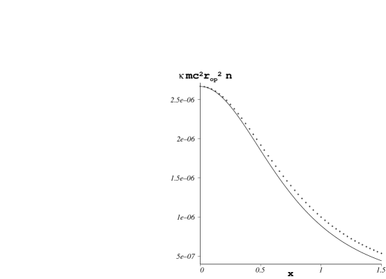
Figure 1: $\underline{\hbox{Comparison of $n$ obtained from (\ref{eq:n11}) and (\ref{eq:n22})}}$. This plot displays the adimensional quantity $\kappa mc^{2}r_{op}^{2}\,n$, as a function of $x$, obtained from truncating the right hand sides of (4.11) (solid curve) and (4.12) (dotted curve with crosses) up to fourth order in $v_{0}/c$ and assuming the consistency condition (4.13). Since we are using an empiric law for observed galactic rotation curves (the URC given by (4.1)), the fact that these two expressions for $n$ are so close to each other provides an empirical justification for the compatibility between MB distribution and these rotation curves.

where $v_{0}$ denotes a velocity ($\hbox{km}/\hbox{sec}$) and not the adimensional ratio $v_{0}/c$. Equation (4.13) is analogous to the condition that defines the so-called “virialized temperature” in the context of cooling of a baryon gas, though in the present approach such a temperature corresponds to the dark matter gas (see section 17.3 of [3]). Since higher order terms in $v_{0}/c$ have a minor contribution, the two forms of $n$ are approximately equal. This is shown in Figure 1 displaying the adimensional quantity $\kappa\,mc^{2}n\,r_{\hbox{\tiny{opt}}}^{2}$ from (4.11) and (4.12) as functions of $x$ for typical values $v_{0}=200\,\hbox{km/sec},\,a=1$ and eliminating $T_{c}$ with (4.13). Equation (4.6) shows how “flattened” rotation curves, as obtained from the empiric form (4.1), lead to $M\propto r^{3}$ for $r\approx 0$ and $M\propto r$ for large $r$. Equations (4.3) to (4.13) represent a relativistic generalization of the “isothermal sphere” that follows as the newtonian limit of an ideal Maxwell-Boltzmann characterized by $\rho\approx mc^{2}n$, $p\ll\rho$ and $T\approx T_{c}$. In fact, using newtonian hydrodynamics we would have obtained only the leading terms of equations (4.3) to (4.13). It is still interesting to find out that the isothermal sphere can be obtained from General Relativity in the limit $v_{0}/c\ll 1$ by demanding that rotation curves have a form like (4.1). The total mass of the galactic halo, usualy given as $M$ evaluated at the radius $r=r_{200}$ (the radius at which $\rho$ is 200 times the mean cosmic density). Assuming this density to be $\approx 10^{-29}\,\hbox{gm}/\hbox{cm}^{3}$ together with typical values $v_{0}=200\,\hbox{km}/\hbox{sec}$ and $a=1$ yields $r_{200}\approx 150$ kpc. Evaluating $M$ at this values yields about $10^{17}\,M_{\odot}$, while $M$ evaluated at a typical $r_{opt}=15$ kpc leads to about $10^{12}\,M_{\odot}$, an order of magnitude larger than the galactic mass due to visible matter. These values are consistent with Refs. [30] and [31].

5 Discussion.

So far we have found a reasonable approximation for galactic dark matter to be described by a self gravitating Maxwell-Boltzmann gas, under the assumption of the empiric rotation velocity law (4.1). The following consistency relations emerge from equations (4.11), (4.12) and (4.13)

$$n_{c}\ \approx\ \frac{3\,v_{0}^{2}}{4\pi G\,m\,a^{2}\,r_{\hbox{\tiny{opt}}}^{2}},\qquad T_{c}\ \approx\ \frac{m\,v_{0}^{2}}{3\,k_{{}_{B}}}$$ (5.1)

hence, bearing in mind that $n\leq n_{c}$ and $T\approx T_{c}$, the condition (3.1) for the validity of the MB distribution can be written as

$$\frac{n\,\hbar^{3}}{(m\,k_{{}_{B}}\,T)^{3/2}}\ \leq\ \frac{n_{c}\,\hbar^{3}}{(m\,k_{{}_{B}}\,T_{c})^{3/2}}\ \ll\ 1,$$ (5.2)

Inserting (5.1) into (5.2) yields the condition

$$m\ \gg\ \left[\frac{3^{5/2}\,\hbar^{3}}{4\pi G\,a^{2}\,r_{\hbox{\tiny{opt}}}^{2}\,v_{0}}\right]^{1/4},$$ (5.3)

a criteria of aplicability of the MB distribution (non-degeneracy) that is entirely given in terms of $m$, the fundamental constants $G,\,\hbar$ and the empiric parameters $v_{0}$ and $b\equiv a\,r_{\hbox{\tiny{opt}}}$ (the “terminal” rotation velocity and the “core radius”). For dark matter dominated galaxies (spiral and low surface brightness (LSB)) [30] these parameters have a small variation range: $r_{\hbox{\tiny{opt}}}\approx 15$ kpc , $1$ kpc   $\leq b\leq$   5 kpc and $125\,\hbox{km/sec}\leq v_{0}\leq 250\,\hbox{km/sec}$, the constraint (5.3) does provide a tight estimate of the minimal value for the mass of the particles under the assumption that these particles form a self gravitating ideal dark gas complying with MB statistics. As shown in Figure 2, this minimal value lies between $30$ and $60$ eV, thus implying that appropriate particle candidates must have a much larger mass than this range of values. This minimal bound excludes, for instance, light mass particles such as the electron neutrino ($m_{\nu_{e}}<2.2$ eV) or the axion ($m_{A}\approx 10^{-5}$ eV). The currently accepted estimations of cosmological bounds on the sum of masses for the three active neutrino species is about $24$ eV [28], a value that would apparently rule out all neutrino flavours. However, recent estimations of these cosmological bounds have raised this sum to about $1$ keV [42], hence more massive neutrinos could also be accomodated as dark matter particle candidates. Estimates of masses of various particle candidates are displayed in Table 1.

Since $T\approx T_{c}$, the consistency condition (4.13) provides the following constraint on the temperature and particles mass of the dark gas

$$\frac{m}{T_{c}}\ =\ \frac{3\,k_{{}_{B}}}{v_{0}^{2}}\ \approx 0.4\times 10^{3}\,\frac{\hbox{eV}}{\hbox{K}}\ ,$$ (5.4)

where we have taken $v_{0}=200\,\hbox{km/sec}$ . Considering in (5.4) the minimal mass range that follows from (5.3), we would obtain gas temperatures consistent with the assumed typical temperatures of relic gases: $T_{c}\approx 2\,\,\hbox{to}\,\,4\,\hbox{K}$. However, as long as we do not have more information on the interaction and physical properties of various particle candidates, we cannot rule out a given large mass value on the grounds that the corresponding gas temperature could be too high. However, if we assume that the ideal dark gas is made of electrons or barions, so that $m=m_{p}$ or $m=m_{e}$, then condition (5.3) for applicability of the MB distribution is certainly satisfied, but (5.4) implies a temperature of the order of $T_{c}\approx 10^{3}$ K for electrons and $T_{c}\approx 10^{6}$ K for barions ! Obviuosly, barions or electrons at such a high temperatures would certainly not remain unobservably “dark”. We can rule them out, but we cannot rule out more massive particles (in the range of 1-100 GeV’s) characterized by weak interaction even if the gas temperature is in the range of $10^{8}-10^{9}$ K. Figure 3 illustrates, for various particle candidates, the relation between $T_{c}$ and $m$ contained in (5.4). The main novelty of the present paper is the fact that it is based on a general relativistic hydrodynamics, as opposed to numerical simulations [7]-[9], newtonian or Kinetic Theory perturbative approaches (see [12]-[22]).

Finaly, the fact that under the assumption of MB distribution, we have obtained a minimal mass on the range $30\,\hbox{eV}\leq m\leq 60\,\hbox{eV}$ that seems to discriminate against thermal relique gases composed by lighter particles (electron neutrino, etc) coincides with the fact that these particle candidates tend to be ruled out because of their inability to produce sufficient matter clustering [2], [3]. In spite of these arguments, if either of these particles constitute a self gravitating gases accounting for a galactic halo it would be inconsistent to model such a gas as SCDM in the context of a classical ideal gas complying with MB statistics. It would be necessary to examine these cases as either HDM or WDM, by using either a relativistic MB distribution (very light particles can be relativistic even at low temperatures) and/or a distribution that takes into account (depending on the particle) Fermi-Dirac or Bose-Einstein statistics. Non-thermal axions are very light particles ($m\sim 10^{-5}$ eV), however this type of relique source cannot be treated as a Maxwell-Boltzmann gas, thus the lower mass limit that we have obtained does not apply. This and other non-thermal sources [23, 24] require a wholy different approach. These studies will be undertaken in future papers.

SCDM/WDM	mass in keV	References
Light Candidates
Light Gravitino	$\sim 0.5$	[35]
	$\sim 0.75-1.5$	[36], [37]
	$\sim 2.6-5$	[38]
Sterile Neutrino	$<40$	[39]
	$1-100$	[40]
Standard Neutrinos	$\sim 1$	[41], [42]
Dilaton	$\sim 0.5$	[43]
Light Axino	$\sim 100$	[44]
Majoron	$\sim 1$	[45], [46], [47]
Mirror Neutrinos	$\sim 1$	[48], [49]
CDM	mass in GeV	References
Heavy Candidates
Neutralino	$>32.3$	[50]
	$>46$	[51]
Axino	$\sim 10$	[52], [53]
Gravitino	${\buildrel<\over{\sim}}\ 100$	[54]

Table 1: Particle candidates for a MB Dark Matter gas.

6 Acknowledgments

We thank Professor Rabindra N. Mohapatra for calling our attention to the important papers of Ref. [15] and [16] and N. Fornengo for useful discussions. R. A. S. is partly supported by the DGAPA-UNAM, under grant (Project No. IN122498), T. M. is partly supported by CoNaCyT México, under grant (Project No. 34407-E) and L. G. C. R. has been supported in part by the DGAPA-UNAM under grant (Project No. IN109001) and in part by the CoNaCyT under grant (Project No. I37307-E).

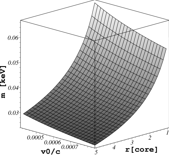
Figure 2: $\underline{\hbox{Minimal mass for which the Maxwell-Boltzmann distribution is applicable}}$. This graph displays $m$ (in keV’s) as a function of $v_{0}/c$ and $b=a\,x$, respectively, the terminal velocity and ‘halo core radius’ associated with the URC given in (4.1). Assuming typical ranges for spiral galaxies: $125\,\hbox{km/sec}\leq v_{0}\leq 250\,\hbox{km/sec}$ and $1\,\hbox{kpc}\leq b\leq 5\,\hbox{kpc}$, we obtain masses in the range of $30\,\hbox{eV}\leq m\leq 60\,\hbox{eV}$ that follow from the right hand side of the relation (5.3), providing the criterion for applicability of the Maxwell-Bolzmann distribution. Dark matter particle candidates complying with an MB distribution must have much larger mass than the plotted values  $30\,\hbox{eV}\leq m\leq 60\,\hbox{eV}$.

Figure 3: $\underline{\hbox{Relation between particle mass and central temperature}}$. This graph displays the relation between $\log_{10}(T_{c})$ (in K) and $\log_{10}(m)$ (in keV’s) that follows from equation (5.4) for a terminal velocity $v_{0}=200\,\hbox{km/sec}$. Almost identical plots are obtained for other velocities in the observed range $125\,\hbox{km/sec}\leq v_{0}\leq 250\,\hbox{km/sec}$. The circle and box symbols respectively denote the proton and electron mass yielding central temperatures of the order $T_{c}\approx 10^{6},\,10^{3}$ K. The central temperature for light particles in the range $0.5\,\hbox{keV}\leq m\leq 100\,\hbox{keV}$ is less than $300$ K (rectangle in the left), while for massive sypersymmetric particles in the range $1\,\hbox{GeV}\leq m\leq 100\,\hbox{GeV}$, we have $T_{c}$ as large as $10^{9}$ K (rectangle on the right). However, such high temperatures cannot rule out these weakly interactive particles as components of the dark matter MB gas.

References

-
[1]
V. Trimble, Ann. Rev. Astron. 25,
425 (1987).
V. Trimble, Contemp. Phys. 29, 373 (1988).
A. D. Dolgov, invited talk at Gamow Memorial International Conference. e-Print Archive: hep-ph/9910532. - [2] T. Padmanabhan, Structure formation in the universe. Cambidge University Press, Cambridge, U.K., (1995).
- [3] C. Peacock, Cosmological Physics, Cambridge University Press, 1999.
- [4] C. Boehm, P. Fayet and R. Schaeffer, astro-ph/0012404.
- [5] P.J.E. Peebles, ApJ, 277, 470, (1984).
- [6] C.S. Frenk et al, ApJ, 327, 507, (1988).
- [7] J.F. Navarro, C.S. Frenk and S.D.M. White, ApJ, 462, 563, (1996); see also: J.F. Navarro, C.S. Frenk and S.D.M. White, ApJ, 490, 493, (1997).
- [8] B. Moore et al, MNRAS, 310, 1147, (1999).
- [9] S. Ghigna et al, astro-ph/9910166.
- [10] B. Moore, Nature, 370, 629, (1994).
- [11] R. Flores and J. P. Primack, ApJ, 427, L1, (1994).
- [12] D.N. Spergel and P.J. Steinhardt, Phys Rev Lett., 84, 3760, (2000).
- [13] A. Burkert, APJ Lett., 534, 143, (2000).
- [14] C. Firmani et al, MNRAS, 315, 29, (2000).
- [15] R.N. Mohapatra, S. Nussinov, V. L. Teplitz. e-Print Archive: hep-ph/0111381.
- [16] Rabindra N. Mohapatra and Vigdor L. Teplitz Phys. Rev. D62, 063506 (2000).
- [17] S. Colombi, S. Dodelson and L. Widrow, ApJ, 458, 1, (1996).
- [18] R. Schaeffer and J. Silk, ApJ, 332, 1, (1998).
- [19] C.J. Hogan, astro-ph/9912549.
- [20] S. Hannestad and R. Scherrer, Phys. Rev. D, 62, 043522, (2000).
- [21] J.J. Dalcanton and C.J. Hogan, astro-ph/0004381.
- [22] C.J. Hogan and J.J. Dalcanton, astro-ph/0002330.
- [23] Tonatiuh Matos and F. Siddhartha Guzmán. Class. Quant. Grav., 17, (2000), L9-L16. Available at: gr-qc/9810028. See also: Tonatiuh Matos and Luis A. Ureña. Phys Rev. D63, (2001), 063506. Available at: astro-ph/0006024.
- [24] Tonatiuh Matos, F. Siddhartha Guzmán and Darío Núñez. Phys Rev. D62, (2000), 061301(R). Available at: astro-ph/0003398. Tonatiuh Matos, Darío Núñez, F. Siddhartha Guzmán and Erandy Ramirez. Gen. Rel. Grav., 34, (2002), in press. Available at: astro-ph/0005528. Tonatiuh Matos and F. Siddhartha Guzmán. Class. Quant. Grav., 18, (2001), 5055-5064. Available at: gr-qc/0108027.
- [25] U. Nucamendi, M. Salgado and D. Sudarsky, Phys. Rev. Lett., 84, 3037, (2000).
- [26] Palash B. Pal, Particle dark matter: an overview, Invited talk at Workshop on Cosmology: Observations Confront Theories, West Bengal, India, 11-17 Jan 1999. Published in Pramana 53: 1053-1059, 1999. e-Print Archive: astro-ph/9906261.
- [27] Q. R. Ahmad, et. al. (SNO Collaboration) Phys. Rev. Lett. 87, 071301 (2001).
- [28] The 2000 Review of Particle Physics (Particle Data Group), D. E. Groom et. al., Eur. Phys. Jour. C15, 1 (2000) and 2001 partial update for edition 2002 (URL: http://pdg.lbl.gov).
- [29] John Ellis, Summary of DARK 2002: 4th International Heidelberg Conference on Dark Matter in Astro and Particle Physics, Cape Town, South Africa, 4-9 Feb. 2002. e-Print Archive: astro-ph/0204059.
- [30] P. Salucci and M. Persic, in Dark and visible matter in galaxies, eds. M. Persic and P. SalucciASP Conference Series, 117, 1, (1997). Available at astro-ph/9703027.
- [31] E. Battaner and E. Florido, The rotation curve of spiral galaxies and its cosmological implications. astro-ph/0010475.
- [32] S.R. de Groot, W.A. van Leeuwen and Ch.G. van Weert, Relativistic Kinetic Theory. Principles and Applications, North Holland Publishing Company, 1980. See pp 46-55.
- [33] R. Maartens, Causal Thermodynamics in Relativity, Lectures given at the Hanno Rund Workshop on Relativity and Thermodynamics, Natal University, Durban, S.A., June 1996. Available at e-Print Archive:astro-ph/9609110.
- [34] L. D. Landau and E. M. Lifshitz Física Estadística, Parte II, Volumen 9 del Curso de Física Teórica, Editorial Reverté, S. A. (1986), see Eq. (4.65).
- [35] M. Kawasaki, N. Sugiyama and T. Yanagida, Mod. Phys. Lett. A12, 1275 (1997).
- [36] E. A. Baltz and H. Murayama, e-Print Archive: astro-ph/0108172.
- [37] S. D. Burns, e-Print Archive:astro-ph/9711304.
- [38] S. H. Hansen, J. Lesgourgues, S. Pastor and J. Silk, e-Print Archive: astro-ph/0106108.
- [39] A. D. Dolgov and S. H. Hansen, e-Print Archive: hep-ph/0009083.
- [40] K. Abazajian, G. M. Fuller and M. Patel, Phys. Rev. D64, 023501 (2001).
- [41] Chun Liu and J. Song, Phys. Lett. B512, 247 (2001).
- [42] G. F. Giudice, E. W. Kolb, A. Riotto, D. V. Semikoz and I. I. Tkachev, Phys. Rev. D64, 043512 (2001).
- [43] Y. M. Cho and Y. Y. Keum, Mod. Phys. Lett. A13, 109 (1998).
- [44] S. A. Bonometto, F. Gabbiani and A. Masiero, Phys. Rev. D49, 3918 (1994).
- [45] V. Berezinsky and J. W. F. Valle, Phys. Lett. B318, 360 (1993).
- [46] K. S. Babu, I. Z. Rothstein and D. Seckel, Nucl. Phys. B403, 725 (1993).
- [47] A. Dolgov, S. Pastor and J. W. F. Valle, e-Print Archive: astro-ph/9506011.
- [48] Z. G. Berezhiani and R. N. Mohapatra, Phys. Rev. D52, 6607 (1995).
- [49] Z. G. Berezhiani, Acta Phys. Polon. B27, 1503 (1996).
- [50] P. Abreu et al. Phys. Lett. B 489, 38-35 (2000).
- [51] J. Ellis, T. Falk, G. Ganis and K. A. Olive Phys. Rev. D 62, 075010 (2000).
- [52] L. Covi, H. B. Kim, J. E. Kim and L. Roszkowski, JHEP 0105, 033 (2001).
- [53] Leszek Roszkowski, invited plenary talk at the 4th International Workshop on Particle Physics and the Early Universe (COSMO-2000), Cheju, Cheju Island, Korea, September 4-8, 2000 and the 3rd International Workshop on the Identification of Dark Matter (IDM-2000), York, England, 18-22 September 2000. e-Print Archive: hep-ph/0102325.
- [54] M. Kawasaki and T. Moroi Prog. Theor. Phys. 93, 879-900 (1995).