The Collapse of Large Extra Dimensions

Abstract

In models of spacetime that are the product of a four-dimensional spacetime with an “extra” dimension, there is the possibility that the extra dimension will collapse to zero size, forming a singularity. We ask whether this collapse is likely to destroy the spacetime. We argue, by an appeal to the four-dimensional cosmic censorship conjecture, that—at least in the case when the extra dimension is homogeneous—such a collapse will lead to a singularity hidden within a black string. We also construct explicit initial data for a spacetime in which such a collapse is guaranteed to occur and show how the formation of a naked singularity is likely avoided.

I Introduction

The idea that we live in a universe with more than the four dimensions we observe has been around for some time. Models of the universe with five or more dimensions, originally proposed by Kaluza and Klein Kaluza (1921); Klein (1926a) as an attempt to unify electromagnetism and general relativity, have been commonplace in string theory for many years. In such theories the extra dimensions typically have a “size” comparable to the Planck length and thus remain unseen since experiments that would reveal their presence require as-yet-unattainable energies. Furthermore, questions about the evolution and stability of the extra dimensions have been largely ignored since at this scale quantum gravity effects are presumably important and it is difficult to extract predictions from any current candidate theory of quantum gravity.

Recently, however, there has been a great deal of interest in models wherein the size of the extra dimensions is much larger than the Planck length Arkani-Hamed et al. (1998); Antoniadis et al. (1998); Rubakov (2001). Current experimental results involving tests of the inverse square law (see, e.g., Hoyle et al. Hoyle et al. (2001)) do not rule out extra dimensions even as large as a tenth of a millimeter. It is now important to consider the evolution of the extra dimensions since the observed strength of the gravitational force is directly dependent on the size of the extra dimensions. Furthermore, since the curvature of spacetime is now much larger than Planckian scales it ought to be possible to study the evolution of such spacetimes within the framework of classical general relativity.

As an example, consider a spacetime whose manifold is the product of four-dimensional Minkowski spacetime with a single extra dimension of topology $S^{1}$ and whose metric is

$$ds^{2}=\eta_{\mu\nu}\,dx^{\mu}\,dx^{\nu}+b(t)^{2}d\psi^{2}.$$

Here $\eta_{\mu\nu}$ is the metric of Minkowski spacetime, $x^{\mu}$ are the coordinates in “usual” dimensions, $\psi$ is the coordinate in the fifth dimension, and $b(t)$ is the scale of the extra dimension. It is clear that that this metric is a solution to Einstein’s equation when $b(t)$ is constant, say $b(t)=b_{0}$, since the spacetime is then flat. However, it is easy to check that a solution is also obtained by setting $b(t)=b_{0}+\alpha t$, with $\alpha$ a constant. If $\alpha$ is negative, then clearly the extra dimensions will collapse to zero size—and the whole spacetime will become singular—in finite time. Although this model is rather unrealistic in that the scale factor of the extra dimension is the same, and evolving in the same manner, throughout the entire space, we shall show in section III that it is possible to construct more realistic examples in which the collapse happens locally (i.e., within some compact spatial region) and is guaranteed to produce a singularity.

There do exist models in which the size of the extra dimensions is stabilized, at least under small perturbations, by the addition of suitable matter Goldberger and Wise (1999); Randall and Sundrum (1999a); Günther and Zhuk (2000); Carroll et al. (2001); Arkani-Hamed et al. (2001). However, it is still not clear whether any of these models would describe our universe if extra-dimensional models were taken seriously. Thus one must be concerned about the possibility of singularity formation in the fashion described above and the nature of the singularity so formed. It would be disastrous, for example, if a singularity, once formed, were to propagate outwards from its origin, destroying the spacetime.

Nonetheless, we shall argue that, under reasonable assumptions, a space that is the metric product of a three-dimensional space and an homogeneous, one-dimensional manifold, in which the scale-factor of the extra dimension is collapsing to zero in some region, will evolve to a “black string;” that is, a spacetime that is the metric product of a four-dimensional black-hole spacetime with the extra-dimensional manifold. That is, even if a singularity is formed by extra-dimensional collapse, it will be hidden within an event horizon. To give some insight into the mechanism by which this occurs, we also give an explicit example of a collapsing spacetime and try to make plausible its subsequent evolution into a black string.

Our argument relies on the cosmic censorship conjecture in four space-time dimensions. This conjecture asserts, roughly, that all singularities are hidden inside an event horizon rather than being “naked,” i.e., visible to distant observers; or, in other words, that black holes are the generic final states of gravitational collapse. Although it has not been proven, the cosmic censorship conjecture is widely believed to be true for generic initial conditions.

Ten years ago, Gregory and Laflamme Gregory and Laflamme (1993) showed that black strings are, in fact, unstable to linear perturbations, at least when the scale of the extra dimensions is large enough. If this instability is a true, non-linear instability, the question then arises as to what the final state will be. Gregory and Laflamme suggested that the black string would “fragment” into a chain of black holes, although, since this would require the event horizon to bifurcate (a process that is forbidden if five-dimensional cosmic censorship holds), a naked singularity would result. Thus there is something of a puzzle as to what the final state actually is: if one imposes the symmetry constraint that we do, the final state appears to be a black string; if one does not, then a naked singularity appears to be possible. It has also been suggested Horowitz and Maeda (2001) that the instability will not lead to a bifurcation of the event horizon and that, instead, the spacetime evolves to a stable solution that does not have translational symmetry in the extra dimension.

The outline of this paper is as follows: In section II we describe the cosmic censorship conjecture and the conditions under which it is believed to hold. We then rewrite Einstein’s equation for the five-dimensional spacetime as a four-dimensional theory with an effective matter content and show that this effective matter content does indeed satisfy the conditions of the cosmic censorship conjecture. In section III we show how it is in principle possible to construct initial data that is guaranteed to form a singularity and then give, explicitly, a class of such initial data. By considering a plausible scenario for the evolution of this data, we illustrate how the black string likely arises.

II A General Argument from the Cosmic Censorship Conjecture

In the Introduction we gave a simple example of a spacetime possessing an extra dimension in which the extra dimension collapses to zero size everywhere on a spacelike surface and the worldline of every observer ends on the singularity in finite proper time. In this section we argue that such a catastrophic fate will not befall more realistic examples and that even a naked singularity will not occur, provided that the extra dimension is homogeneous.

In order to proceed, we shall make the simplifying assumption that the spacetime is the product of a four-dimensional manifold, $M$, with $S^{1}$ (though it makes no difference to our argument if the extra dimension has the topology of $\mathbb{R}$) and that the metric of the full spacetime, ${}^{(5)}g_{AB}$ can be written in the form

$$ds^{2}={}^{(5)}g_{AB}\,dx^{A}dx^{B}=g_{ab}(x)dx^{a}dx^{b}+e^{2\sqrt{2/3}\,\beta(x)}\,d\psi^{2},$$ (1)

where the $x^{a}$ are coordinates in the “ordinary,” four-dimensional, spacetime, $\psi$ the coordinate in the extra dimension, and we shall use uppercase Roman letters to denote indices in the full, five-dimensional spacetime but lowercase Roman letters for indices in the four-dimensional spacetime.

The four-dimensional metric $g_{ab}$, and the scale factor $\beta(x)$, do not depend upon $\psi$ but are otherwise completely general. That is, we consider only spacetimes in which the extra dimension is homogeneous. This form of the metric is typical of many models considered in the literature and is similar to the original Kaluza-Klein ansatz except that we disallow off-diagonal terms in the metric.

Einstein’s equation in the full spacetime, in geometric units (where $G=c=1$), is

$${}^{(5)}G_{AB}=8\pi{}^{(5)}T_{AB},$$ (2)

where ${}^{(5)}G_{AB}$ is the five-dimensional Einstein tensor, and ${}^{(5)}T_{AB}$ the five-dimensional stress-energy tensor. Note that to be consistent with the form of ${}^{(5)}g_{AB}$ given above we must impose the condition ${}^{(5)}T_{a\psi}=0$ on the stress-energy.

Our approach will be to show that this equation may be rewritten as the equations describing four-dimensional relativity with the addition of a scalar field, and hence to argue that the four-dimensional cosmic censorship conjecture precludes the existence of either a naked singularity or a spacetime-destroying one. This “dimensional reduction” is usually carried out in a Lagrangian formulation (see, for example, the survey article by Overduin and Wesson Overduin and Wesson (1997) and references therein) but we shall instead directly rewrite Einstein’s equation to arrive at a four-dimensional theory with some effective stress-energy tensor. Rewriting Einstein’s equation in this way has the benefit that it is more straightforward to determine the effective stress-energy tensor—particularly when the matter content does not have a Lagrangian formulation—and, furthermore, one can be sure of obtaining all the equations of motion.

II.1 Dimensional Reduction

From our metric ansatz, eq. (1), we can rewrite the five-dimensional tensors appearing in the theory in terms of their four-dimensional counterparts. We find,

$$\begin{split}{}^{(5)}R_{ab}&=R_{ab}[g_{ab}]-\frac{2}{3}D_{a}\beta D_{b}\beta-\sqrt{\frac{2}{3}}D_{a}D_{b}\beta,\\ {}^{(5)}R_{\psi\psi}&=-e^{2\sqrt{2/3}\,\beta}\Bigl{(}\frac{2}{3}D^{a}\beta D_{a}\beta+\sqrt{\frac{2}{3}}D^{a}D_{a}\beta\Bigr{)}.\end{split}$$ (3)

Here ${}^{(5)}R_{ab}$ is the five-dimensional Ricci tensor projected into the four-dimensional space and $R_{ab}[g_{ab}]$ is the Ricci tensor associated with the four-dimensional part of the metric, $g_{ab}$. (The mixed-index terms, ${}^{(5)}R_{a\psi}$, are zero.) Finally, $D_{a}$ is the derivative operator associated with $g_{ab}$. Using the above we can rewrite the Einstein tensor:

$$\begin{split}{}^{(5)}G_{ab}&={}^{(5)}R_{ab}-\frac{1}{2}{}^{(5)}R{}^{(5)}g_{ab}\\ &=G_{ab}-\Bigl{[}\frac{2}{3}D^{a}\beta D_{a}\beta+\sqrt{\frac{2}{3}}D^{a}D_{a}\beta\Bigr{]}\\ &\qquad\qquad+\Bigl{[}\frac{2}{3}D^{a}\beta D_{a}\beta+\sqrt{\frac{2}{3}}D^{a}D_{a}\beta\Bigr{]}g_{ab},\\ {}^{(5)}G_{\psi\psi}&=-\frac{1}{2}Re^{2\sqrt{2/3}\,\beta}.\end{split}$$ (4)

where $R=R_{ab}g^{ab}$ and $G_{ab}=R_{ab}-\frac{1}{2}Rg_{ab}$.

One could at this point equate the right hand side of the first equation above to the four-dimensional part of the stress-energy tensor and consider the expression involving $\beta$ as part of an effective stress-energy. However, this expression is not recognizable as the stress-energy of, say, a scalar field. To rewrite the equation so that the stress-energy is recognizable, we make the conformal transformation

$$g_{ab}=e^{-\sqrt{2/3}\,\beta}\tilde{g}_{ab}.$$ (5)

The Ricci tensor and scalar then become

$$\begin{split}R_{ab}&=\tilde{R}_{ab}[\tilde{g}_{ab}]+\frac{1}{3}\tilde{D}_{a}\beta\tilde{D}_{b}\beta+\sqrt{\frac{2}{3}}\tilde{D}_{a}\tilde{D}_{b}\beta\\ &\qquad+\frac{1}{2}\Bigl{[}\sqrt{\frac{2}{3}}\tilde{D}^{c}\tilde{D}_{c}\beta-\frac{2}{3}\tilde{D}^{c}\beta\tilde{D}_{c}\beta\Bigr{]}\tilde{g}_{ab},\\ R&=e^{\sqrt{2/3}\,\beta}\Bigl{[}\tilde{R}+3\sqrt{\frac{2}{3}}\tilde{D}^{c}\tilde{D}_{c}\beta-\tilde{D}^{c}\beta\tilde{D}_{c}\beta\Bigr{]},\\ \end{split}$$ (6)

where now $\tilde{D}_{a}$ is the derivative operator associated with $\tilde{g}_{ab}$ and indices are raised and lowered with $\tilde{g}_{ab}$. Finally, we substitute this expression for $R_{ab}$ into eq. (4) and also replace $D_{a}$ by $\tilde{D}_{a}$ there, to obtain

$$\begin{split}{}^{(5)}G_{ab}&=\tilde{G}_{ab}-\tilde{D}_{a}\beta\tilde{D}_{b}\beta+\frac{1}{2}(\tilde{D}^{c}\beta\tilde{D}_{c}\beta)\tilde{g}_{ab},\\ {}^{(5)}G_{\psi\psi}&=-\frac{1}{2}e^{3\sqrt{2/3}\,\beta}\Bigl{[}\tilde{R}+3\sqrt{\frac{2}{3}}\tilde{D}^{c}\tilde{D}_{c}\beta-\tilde{D}^{c}\beta\tilde{D}_{c}\beta\Bigr{]}.\end{split}$$ (7)

Thus, from Einstein’s equation in the full spacetime, eq. (2), we have,

$$\begin{split}\tilde{G}_{ab}&=8\pi{}^{(5)}T_{ab}+\tilde{D}_{a}\beta\tilde{D}_{b}\beta-\frac{1}{2}(\tilde{D}^{c}\beta\tilde{D}_{c}\beta)\tilde{g}_{ab},\\ \tilde{D}^{a}\tilde{D}_{a}\beta&=-\sqrt{\frac{2}{3}}e^{-3\sqrt{2/3}\,\beta}{}^{(5)}T_{\psi\psi}+\frac{1}{\sqrt{6}}\tilde{g}^{ab}{}^{(5)}T_{ab},\end{split}$$ (8)

One may interpret this as the theory of General Relativity in four dimensions, with matter content described by ${}^{(5)}T_{ab}$, plus a massless scalar field, $\beta$, coupled to ${}^{(5)}T_{ab}$ and ${}^{(5)}T_{\psi\psi}$.

We now discuss the cosmic censorship conjecture.

II.2 The Cosmic Censorship Conjecture

It is widely believed that in a four-dimensional spacetime arising from reasonable initial data, with reasonable matter content, no singularities will be visible to distant observers; that is, all singularities will be hidden within black holes. (See, e.g., Wald Wald (1997) for a survey of past and recent results.) Here we recall the precise statement of this conjecture by giving a meaning to the notion of “reasonable” initial data, “reasonable” matter, and “distant observers,” and hence argue that the singularity formed by a collapsing extra dimension will likewise be hidden, given the results of section II.1.

We first say what is meant by a distant observer. The intuitive meaning is an observer located “far away, in the future” where the spacetime “looks like” flat spacetime. The precise meaning for these terms is given by the notion of asymptotic flatness at future null infinity. Roughly speaking, future null infinity, $\mathcal{I}^{+}$, is the “endpoint” of null geodesics that propagate out to large distances. (The details of this construction, which are not important here, can be found in advanced textbooks on general relativity (Wald, 1984, Chapter 11).) If the spacetime is asymptotically flat at future null infinity then it “looks like” flat spacetime at sufficiently large distances and late times; $\mathcal{I}^{+}$ then represents “far away in the future.” The notion that a distant observer will be able to avoid running into a singularity is then captured by the precise statement that future null infinity is complete. Furthermore, if no past-directed causal curve from $\mathcal{I}^{+}$ terminates at a singularity, then distant observers will not be able to see the singularity.

Next we explain what sort of initial data we allow. Clearly no version of the cosmic censorship conjecture will hold without some restriction on the initial data: for example, the spacetime given in the Introduction does produce a spacetime-destroying singularity. On the other hand, if one lives in a spacetime that is not, initially, collapsing everywhere, one cannot create such initial collapse because the collapse is not confined to some compact region. We thus wish to require that at large distances the initial data approaches flat space. It turns out that a notion of asymptotic flatness may be defined for initial data sets, analogous to asymptotic flatness at future null infinity for spacetimes, and we will allow only asymptotically flat initial data.

Finally, for the purposes of the conjecture, the matter content must be “well-behaved” in the following sense:

1. The coupled Einstein-matter equations have a well-posed initial value formulation;

2. The matter satisfies the dominant energy condition so that observers do not see negative energy densities or “superluminal” energy flow; and

3. The matter is not of such a nature as to produce singularities in a fixed, non-singular, background spacetime, uncoupled from Einstein’s equation.

We now state one version of the cosmic censorship conjecture.

Weak Cosmic Censorship Conjecture: Consider asymptotically flat initial data for Einstein’s equation with suitable matter, in the sense given above. Then, generically, the maximal Cauchy evolution of this data is a spacetime that is asymptotically flat at future null infinity, with complete $\mathcal{I}^{+}$.

II.3 Application to Extra-Dimensional Spacetimes

If the extra dimension collapses in the evolution of a five-dimensional spacetime whose metric is of the form (1) then a singularity will be produced. In the conformally transformed, four-dimensional theory, this singularity appears as a divergence of the scalar field and, in particular, a divergence of the stress-energy of the scalar field. Thus, there will also be a space-time singularity in the four-dimensional theory. However, we are now in a position to argue that this singularity will be contained within a black hole.

Thus, consider a five-dimensional spacetime for which the five-dimensional matter content satisfies conditions 1–3 above and such that the initial data for the equivalent four-dimensional spacetime is asymptotically flat; then, assuming that the cosmic censorship conjecture is true, we claim that the singularity will be contained within a black hole (a black string in the five dimensional theory).

To see that this is true, let there be given initial data for the five-dimensional spacetime and hence, by the equivalence described in section II.1, we obtain initial data for a four-dimensional spacetime with matter content that includes a scalar field. Now to show that the cosmic censorship conjecture applies to the four-dimensional initial data we must show that the four-dimensional matter content is well-behaved in the sense above. It is well-known that a massless scalar field is well-behaved. Since, by assumption, the five-dimensional equations have a well-posed initial value formulation it is clear that the four-dimensional equations will also, for they are just a rewriting of the five-dimensional equations.

Likewise, note that the evolution of this matter from non-singular initial data in a fixed background with fixed $\beta$ is equivalent to that obtained by fixing the five-dimensional background spacetime and thus will not produce a singularity. To satisfy condition 3 above we should actually fix only the four-dimensional spacetime whilst allowing both the matter and $\beta$ to evolve; but this is not equivalent, in the five-dimensional view, to fixing the five-dimensional background spacetime. However, noting that $\beta$ is, on its own, well-behaved, we would expect that, were we also to allow $\beta$ to evolve, a singularity would not arise. Thus, it appears highly plausible that condition 3 does hold for the effective, four-dimensional matter content.

It remains only to check that the four-dimensional stress-energy satisfies the dominant energy condition. To this end, let $\xi^{a}$ be any future-directed, timelike vector (future-directed and timelike with respect to $\tilde{g}_{ab}$). We must shown that the vector $-\xi_{a}T_{bc}\tilde{g}^{ab}$ is future-directed timelike or null. But this is true because $\xi^{a}$ is future-directed and timelike with respect to $g_{ab}$, and hence with respect to ${}^{(5)}g_{AB}$, and, by assumption, the dominant energy condition holds with respect to ${}^{(5)}g_{AB}$.

Thus, if the four-dimensional cosmic censorship conjecture holds, the singularity formed in the four-dimensional spacetime with metric $\tilde{g}_{ab}$ will be contained within a black hole.

Now note that the projection of a curve in the five-dimensional spacetime that is timelike (or causal) with respect to ${}^{(5)}g_{AB}$ is a curve in the four-dimensional spacetime that is timelike (or causal) with respect to $\tilde{g}_{ab}$. Thus, a reasonable definition of a “distant observer” in the five-dimensional spacetime would be one whose world-line, when projected into the four-dimensional spacetime, is the world-line of a distant observer there. Then, by the same reasoning, if a distant observer in the five-dimensional spacetime were able to see the singularity, the observer in the four-dimensional spacetime obtained by projecting his worldline would be able to see the singularity also. But we have already argued that the four-dimensional distant observers do not see the singularity and we therefore conclude that the singularity is not visible to distant observers in the full spacetime, either.

II.4 More than One Extra Dimension

To conclude this section, we comment briefly on an obvious generalization of this model to more than one extra dimension. It turns out that in this case the conclusion that the effective matter content satisfies the dominant energy condition does not necessarily hold.

Suppose that there are now $n$ extra dimensions. Previously we required that the scale factor $e^{\beta(x)}$ did not depend on the coordinate of the extra dimension. Likewise here, for simplicity, we shall assume that the extra-dimensional manifold is a maximally symmetric space whose metric depends on position only through a scale factor that varies with position in the “usual” dimensions. The metric then has the form

$$ds^{2}=g_{AB}dx^{A}dx^{B}+e^{\sqrt{\frac{2}{n(n+2)}}\,\beta}\gamma_{\mu\nu}dy^{\mu}dy^{\nu},$$ (9)

where the $y^{\mu}$ are the coordinates in the $n$ extra dimensions and $\gamma_{\mu\nu}$ is the metric of a maximally symmetric manifold. The action for General Relativity in this model may be dimensionally reduced in precisely the same way as shown above for the $n=1$ case producing again an effective four-dimensional theory containing a scalar field. (As in the case of one extra dimension, this reduction is typically done in a Lagrangian picture Carroll et al. (2001); Amendola et al. (1990); Günther and Zhuk (2000).) After dimensional reducing the equations and making the conformal transformation $g_{ab}=e^{-\sqrt{2n/(n+2)}\,\beta}\tilde{g}_{ab}$ the result for the effective stress energy is

$$\begin{split}8\pi T_{ab}&=8\pi{}^{(4+n)}T_{ab}+\tilde{D}_{a}\beta\tilde{D}_{b}\beta\\ &\quad{}-\frac{1}{2}\bigl{(}\tilde{D}^{c}\beta\tilde{D}_{c}\beta-R_{\gamma}e^{-\sqrt{\frac{2(n+2)}{n}}\,\beta}\bigr{)}\tilde{g}_{ab},\end{split}$$ (10)

where $R_{\gamma}$ is the Ricci scalar of $\gamma_{ij}$ and ${}^{(4+n)}T_{ab}$ the four-dimensional projection of the $(4\!+\!n)$-dimensional stress energy. In contrast to the case of one extra dimension, the scalar field part of the stress-energy contains a “potential term” $V(\beta)=-R_{\gamma}e^{-\sqrt{2(n+2)/n}\,\beta}$. The scalar field will satisfy the dominant energy condition if this potential is positive (that is, if the manifold of extra dimensions is negatively curved or flat) but will not do so if the potential is negative; that is, when the manifold of extra dimensions has positive curvature. Typically, in models of extra-dimensional cosmology, a matter term is included in the model (for instance to stabilize the extra dimensions). It may then be the case that the overall effective potential is positive even though the extra dimensions have positive curvature (this is so, for example, in the “monopole” model Arkani-Hamed et al. (2001); Carroll et al. (2001)).

III A Concrete Model of Extra-Dimensional Collapse

In section II we concluded that local extra-dimensional collapse would not give rise to a spacetime-destroying singularity. In the Introduction we gave an example of a spacetime whose extra-dimensional collapse did destroy the universe but in that example the collapse was not initially confined to some local region. In this section we turn the example of the Introduction into a more pertinent one by constructing a class of initial data for spacetimes in which the collapse does occur locally. We then consider this initial data from the four-dimensional point of view.

Under this interpretation the size of the extra dimension appears as a scalar field, constant everywhere on the initial data surface but having non-zero time derivative in the inner region, where, moreover, its value becomes $-\infty$ after finite proper time. Thus, in this picture, the stress-energy in the inner region becomes infinite and hence a singularity forms.

Recall that an outer marginally trapped surface is a spacelike, two-dimensional submanifold that is the boundary of a three-dimensional closed region, such that the expansion of the family of outgoing null geodesics normal to the surface is non-positive. The four-dimensional censorship conjecture implies that any outer marginally trapped surface will be contained within, or coincident with, an event horizon. The event horizon of a stationary black hole, for instance, is an outer marginally trapped surface. From the arguments given in section II, we would, therefore, expect that an outer marginally trapped surface will either exist in the initial data, or be formed sufficiently early to enclose any singularity.

In this section we show how the choice of initial data (within our class of models) that ensures extra-dimensional collapse, also leads one to the conclusion that an outer marginally trapped surface will surround the singularity. In doing so, we gain some insight into the “mechanism” by which the conclusions of section II are enforced.

The idea of our construction is to give initial data that, within some compact region, “looks like” the collapsing initial data given in the Introduction, but is then asymptotically flat outside this region. Inside the region the spacetime does not “know” that the rest of the spacetime has been changed, and the region will be made large enough that collapse will be guaranteed to occur at some point within it before information about that change propagates in. We now make this idea precise.

Let $A$ be a compact subset of the $t=0$ hypersurface of the spacetime described in the Introduction. (The set $A$ will be the “region within which collapse occurs.”) By the future domain of dependence of $A$ we mean the collection of all points $p$ in the spacetime such that every past-directed, inextendible, causal curve through $p$ intersects $A$. We denote the future domain of dependence of $A$ by $D^{+}(A)$. The point of this definition is that properties of the spacetime at some point $p\in D^{+}(A)$ (such as the metric and any matter fields) depend only upon the initial data specified on $A$ since an observer at $p$ cannot “see” any other part of the initial data set. Furthermore, if there is given new initial data having some region $A^{\prime}$ within which the data is the same as that within $A$, then, in the resulting spacetimes, the two regions $D^{+}(A)$ and $D^{+}(A^{\prime})$ will be isometric.

Hence, if the extra dimension collapses to zero size within $D^{+}(A)$ then collapse will also occur within $D^{+}(A^{\prime})$, i.e., we are guaranteed that the collapse will, in fact, occur in the spacetime resulting from the new initial data.

In the next section, we describe initial data having this property. A schematic diagram of the resulting spacetime is shown in Figure 1. The initial data surface is labelled $\Sigma$; there is an inner region in which the space is flat but in which, however, the extra dimension is collapsing uniformly (this is the region equivalent to $A$) where we have chosen the region large enough that we can be sure that the extra dimension reaches zero size within its future domain of dependence.

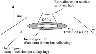
Figure 1: A schematic diagram of the spacetime described in the text. One ordinary spatial dimension and the extra dimension have been suppressed. The initial data surface is labelled $\Sigma$. The initial stress-energy is non-zero only in the shaded region.

It might appear that the construction of such initial data would be almost trivial: one sets the metric to be Minkowski out near infinity; inside some region one sets the metric to be such that the extra dimension is collapsing and then smoothly joins these two regions, allowing the matter content of the spacetime to be determined by Einstein’s equation. However, this procedure would likely result in “unreasonable” matter, having negative energy densities or superluminal energy flow. We shall insist that the matter content satisfy the dominant energy condition (see section III.3) (this is the same condition as that used in section II).

The outline of the remainder of this section is as follows: In section III.1 (and Appendix A) we describe initial data whose extra dimension will collapse to zero size. In sections III.2 and III.3 we write down the conditions that the spacetime will collapse and that the matter does satisfy the dominant energy condition and in section III.4 we give the condition that an outer marginally trapped surface be present in the initial data. Finally, in section III.5 we argue that, even in those cases where the initial data does not contain such a surface, there is good reason to believe that the future evolution will contain an event horizon that will prevent signals from the singularity reaching infinity.

III.1 Initial Data Guaranteed to Collapse

III.1.1 General Considerations

In section II we considered spacetimes whose manifold structure was the metric product of a four-dimensional manifold, $M$, with a circle, such that the metric did not depend on the circle coordinate. Here also we shall only consider spacetimes with this property. Furthermore we suppose that the initial data, and hence the resultant spacetime, is spherically symmetric. We now introduce a convenient coordinate system for such a spacetime.

Since the spacetime is spherically symmetric we introduce coordinates $r$, $\theta$, and $\phi$ in the usual way (so that for any point whose radial coordinate is $r$, the area of the 2-sphere of spherical symmetry containing that point is $4\pi r^{2}$). The coordinate in the extra dimension we again denote by $\psi$.

Assuming that the constant-$r$ surfaces are timelike, the spacetime can now be foliated by four-dimensional (“constant time”) hypersurfaces $\Sigma_{t}$ such that $\nabla_{a}r$ is orthogonal to $\nabla_{a}t$. (That is, a surface invariant both under rotations and translation in the extra dimension is a constant time surface if the integral curves of $\nabla_{a}r$ lie within it.)

If the constant-$r$ surfaces become null (e.g., the $r=2M$ surface in Schwarzschild) this construction is not valid since the normal now lies in the surface and the $t$ and $r$ coordinates become degenerate. Likewise this construction may also fail where $\nabla_{a}r=0$ for then $r$ no longer necessarily identifies uniquely a single constant-$r$ surface. However, in the region of the initial data surface that we give later, neither of these problems arises.

It follows that in this coordinate system the metric may be written,

$$\begin{split}ds^{2}&={}^{(5)}g_{AB}dx^{A}dx^{B}\\ &=-f(r,t)^{2}\,dt^{2}+g(r,t)^{2}\,dr^{2}+r^{2}\,d\Omega^{2}+h(r,t)^{2}\,d\psi^{2}.\end{split}$$ (11)

Here $d\Omega^{2}=d\theta^{2}+\sin^{2}\theta\,d\phi^{2}$ is the spherical part of the metric. In section III.1.2 the functions $f(r,t)$, $g(r,t)$, and $h(r,t)$ will be restricted further by a choice of a class of initial data sets.

Our initial data surface will be $\Sigma=\Sigma_{0}$. The induced metric on $\Sigma$ is clearly,

$$s_{AB}dx^{A}dx^{B}=g(r,t)^{2}\,dr^{2}+r^{2}\,d\Omega^{2}+h(r,t)^{2}\,d\psi^{2}.$$ (12)

Now, letting $n^{A}=-f^{-1}(\partial/\partial t)^{A}$ be the field of unit, timelike vectors orthogonal to $\Sigma$, so that $s_{AB}={}^{(5)}g_{AB}+n_{A}n_{B}$, we compute the extrinsic curvature of $\Sigma$ from the usual formula,

$$K_{AB}=\nabla_{A}n_{B}.$$ (13)

Some algebra gives

$$K_{AB}=-\frac{g\dot{g}}{f}(dr)_{A}(dr)_{B}-\frac{h\dot{h}}{f}(d\psi)_{A}(d\psi)_{B},$$ (14)

where a dot denotes a derivative with respect to $t$.

We shall take the matter to be dust, for simplicity. Such a choice has the advantage that the equation of state is trivial (the pressure is zero) as is the equation of motion (the “dust particles” follow geodesics). The matter stress-energy is then of the form

$${}^{(5)}T_{AB}=\sigma u_{A}u_{B}$$ (15)

for some density $\sigma$ and four-velocity $u^{A}$; for consistency with our metric ansatz, we must assume $u_{\psi}=0$. (We write $\sigma$ for the energy density in the stress-energy of the dust to distinguish it from the initial-data energy density.)

The initial, five-dimensional, energy and current densities, $\rho=T_{AB}n^{A}n^{B}$ and $J_{A}=-h{}_{A}{}^{C}T_{CB}\xi^{B}$ are given by the same expressions as in four dimensions (see, e.g., Wald (Wald, 1984, chapter 10)):

$$16\pi\rho =R_{\mathrm{S}}+(K{}^{A}{}_{A})^{2}-K_{AB}K^{AB},$$ (16)

$$-8\pi J_{A} =D^{B}(K_{AB}-K{}^{C}{}_{C}h_{AB}).$$ (17)

Here $D_{A}$ is the spatial derivative operator (i.e., the derivative operator on $\Sigma$ associated with $s_{AB}$) and $R_{\mathrm{S}}$ is the curvature scalar for $(\Sigma,s_{AB})$. Substituting in the equation above the formula (14) for the extrinsic curvature gives, after some work,

$$16\pi\rho =\frac{2}{r^{2}}\frac{\partial}{\partial r}\left[r(1-g^{-2})\right]-\frac{2}{hgr^{2}}\frac{\partial}{\partial r}\Bigl{(}\frac{r^{2}h^{\prime}}{g}\Bigr{)}+\frac{2\dot{g}\dot{h}}{f^{2}gh},$$ (18)

$$8\pi J_{r} =\frac{\dot{g}}{fghr^{2}}\frac{\partial}{\partial r}(r^{2}h)-\frac{1}{h}\frac{\partial}{\partial r}\Bigl{(}\frac{\dot{h}}{f}\Bigr{)},$$ (19)

where a prime denotes a derivative with respect to $r$. (The radial component of $J_{A}$ we have written $J_{r}$; all the other components are zero.)

III.1.2 A Particular Class of Models

We now construct initial data for a class of spacetimes whose extra dimension is collapsing. For some examples in this class, the extra dimension will be guaranteed to collapse and, by looking for outer marginally trapped surfaces, we shall gain some insight into how distant observers are shielded from the extra-dimensional collapse,

This initial data may be described as follows. The space is spherically symmetric and is divided into three regions: An interior region, $r<r_{1}$, in which the size of the extra dimension is collapsing at a constant rate; a transition region, $r_{1}\leqslant r\leqslant r_{2}$; and an outer region, $r>r_{2}$, that is the metric product of the exterior of the Schwarzschild solution and the extra dimension. In the transition region we shall choose the metric functions to interpolate in a simple way between their values at $r_{1}$ and $r_{2}$.

The particular forms of the metric functions are given in Table 1. As well as $r_{1}$ and $r_{2}$, three other parameters determine the initial data: $h_{0}$, the initial size of the extra dimension (which is everywhere the same); $v_{0}$, the initial speed of the collapse of the extra dimension in the interior region; and $M$, the mass per unit length. For convenience, we give, instead of the metric function $g(r)$, a function $q(r)$, where

$$g(r)=\Bigl{(}1-\frac{q(r)}{r}\Bigr{)}^{-1/2}.$$ (20)

(When we do not write the $t$ argument for the metric functions, we mean their initial values at $t=0$; thus $q(r)=q(r,t=0)$ and so forth.)

At $t=0$	$r<r_{1}$	$r_{1}<r<r_{2}$	$r>r_{2}$
$q(r)$	0	$\displaystyle 2M\frac{r-r_{1}}{r_{2}-r_{1}}$	$2M$
$f(r)$	$(1-2M/r_{2})^{1/2}$	$(1-2M/r_{2})^{1/2}$	$(1-2M/r)^{1/2}$
$h(r)$	$h_{0}$	$h_{0}$	$h_{0}$
$\dot{h}(r)$	$-v_{0}$	$\displaystyle-v_{0}\frac{r_{2}-r}{r_{2}-r_{1}}$	0
$16\pi\rho(r)$	0	$4M/[r^{2}(r_{2}-r_{1})]$	0
$8\pi j_{r}(r)$	0	$\displaystyle-\frac{v_{0}}{h_{0}}(1-2M/r_{2})^{-1/2}(r_{2}-r_{1})^{-1}$	0
$8\pi(J^{a}J_{a})^{1/2}=8\pi g^{-1}j_{r}$	0	$\displaystyle-\frac{v_{0}}{h_{0}(r_{2}-r_{1})}\biggl{[}1-\frac{2M}{r}\frac{r-r_{1}}{r_{2}-r_{1}}\biggr{]}^{1/2}\biggl{(}1-\frac{2M}{r_{2}}\biggr{)}^{-1/2}$	0

Table 1: Initial data for the metric functions and matter content of the spacetime described in the text.

Note that the metric functions are continuous, though not smooth, across the boundaries at $r=r_{1}$ and $r=r_{2}$. In Appendix A we show that the corners may be rounded off so that the metric is smooth everywhere, without affecting the conclusions.

In the next two sections we describe the conditions our initial data is supposed to satisfy: that collapse of the extra dimension be guaranteed to occur and that the matter content satisfy the dominant energy condition. It turns out to be convenient to introduce a dimensionless measure of how fast the collapse of the extra dimension is occurring; namely,

$$\gamma\equiv v_{0}r_{1}g_{0}/(h_{0}f_{0}).$$ (21)

Without loss of generality, one could also set $r_{1}=1$ (though we shall not do so) so that our class of spacetimes is described by just three parameters: $M$, $r_{2}$, and $\gamma$.

III.2 Collapse

The collapse will be guaranteed if it occurs within $D^{+}(A)$. The boundary of $D^{+}(A)$ is defined by null rays emitted from the edge of the inner region, $r=r_{1}$, at coordinate time $t=0$, and these will reach $r=0$ at coordinate time $t=r_{1}/f$. Thus if the extra dimension reaches zero size at $r=0$ before this time it cannot be prevented; since the collapse occurs at $t=h_{0}/v_{0}$ we must have

$$\frac{h_{0}}{v_{0}}<\frac{r_{1}}{f},$$ (22)

or equivalently,

$$\gamma>1.$$ (23)

(The collapse of the extra dimension might still occur even if this condition is not satisfied, it is just that it will not occur in $D^{+}(A)$ and thus cannot be guaranteed.)

III.3 Dominant Energy Condition

Recall that the dominant energy condition requires that the stress-energy, $T_{ab}$, be such that, for all future directed, timelike vectors $t^{a}$, the vector $-T{}^{a}{}_{b}t^{b}$ is a future-directed timelike or null vector. For dust, with five-dimensional stress-energy ${}^{(5)}T_{ab}=\sigma u^{a}u^{b}$, this condition is equivalent to requiring that $\sigma\geqslant 0$ and that $u^{a}$ is timelike which, in turn, is equivalent to $\rho^{2}\geqslant J_{a}J^{a}$. When applied to our initial data the condition is

$$\frac{2M}{r^{2}}\geqslant\frac{\gamma}{r_{1}}\left[1-\Bigl{(}\frac{2M}{r_{2}-r_{1}}\Bigr{)}\Bigl{(}\frac{r-r_{1}}{r}\Bigr{)}\right]^{\frac{1}{2}},$$ (24)

and this must be true for all $r$ in the range $r_{1}\leqslant r\leqslant r_{2}$.

III.4 Trapped Surfaces

Up to this point we have been working with the full, five-dimensional spacetime, in part because it was easy to decide when collapse of the extra dimension was inevitable. However, our arguments are based on the four-dimensional cosmic censorship conjecture so, now, consider what the initial data looks like in the dimensionally reduced, conformally transformed picture described in section II.1. We now derive the condition that no outer marginally trapped surfaces exist in the initial data.

In fact, it is sufficient to consider only surfaces of constant $r$-coordinate for the following reason: If any outer marginally trapped surfaces exist, consider the union of all the regions bounded by such surfaces. The boundary of this region, which must be spherically symmetric, is also an outer marginally trapped surface (Wald, 1984, Chapter 12). Thus, if any outer marginally trapped surface exists, a spherically symmetric marginally trapped surface exists.

On a constant-$r$ surface, the induced metric is $\tilde{\omega}_{ab}dx^{a}dx^{b}=h(r)r^{2}d\Omega^{2}$, where the factor of $h(r)$ comes from the conformal transformation. The outgoing, future directed, null vector field $\xi^{a}$ normal to the surface is

$$\xi^{a}=h^{-1/2}f^{-1}\bigl{(}\frac{\partial}{\partial t}\bigr{)}^{a}+h^{-1/2}g^{-1}\bigl{(}\frac{\partial}{\partial r}\bigr{)}^{a}.$$ (25)

Hence the expansion, $\theta$, of the geodesics tangent to this vector field is

$$\theta=\frac{1}{2}\tilde{\omega}^{ab}\pounds_{\xi}\tilde{\omega}_{ab}=h^{-1/2}\Bigl{(}g^{-1}\frac{2}{r}+f^{-1}\frac{\dot{h}}{h}+g^{-1}\frac{h^{\prime}}{h}\Bigr{)}.$$ (26)

On substituting in our forms for $f$, $g$, and $\dot{h}$, and requiring $\theta>0$, we find that the condition that there are no outer marginally trapped surfaces is:

$$\frac{2}{r}\biggl{[}1-\Bigl{(}\frac{2M}{r_{2}-r_{1}}\Bigr{)}\Bigl{(}\frac{r-r_{1}}{r}\Bigr{)}\biggr{]}^{1/2}>\bigl{(}\frac{\gamma}{r_{1}}\bigr{)}\bigl{(}\frac{r_{2}-r}{r_{2}-r_{1}}\bigr{)},$$ (27)

where the inequality must hold for all $r$ such that $r_{1}\leqslant r\leqslant r_{2}$.

III.5 Visibility of the Singularity

We now consider the question: are there any values of the parameters of our model for which conditions (23), (24), and (27) hold? That is, is there an example for which the collapse occurs, the dominant energy condition is satisfied, and there are no outer marginally trapped surfaces? If there is not, these examples will illustrate very clearly how naked singularities are avoided in extra-dimensional collapse; if there is, we shall consider whether such a surface is likely to form around the singularity in the subsequent evolution of the spacetime.

Consider these conditions when $r=r_{1}$. We require $\gamma>1$ to guarantee that the collapse occurs, whilst the condition that there be no outer marginally trapped surfaces reduces to $\gamma<2$. Thus, without even considering the rest of the spacetime, some of the parameters of the model are already severely restricted by requiring that the collapse not cause the formation of an outer marginally trapped surface.

Next consider the conditions at $r=r_{2}$. We obtain $2M/r_{2}<1$ from the condition that there be no outer marginally trapped surfaces, whereas from the dominant energy condition one can obtain $2M/r_{2}\gtrsim 0.6\gamma^{2}(r_{2}/r_{1})^{2}$. Thus there are also severe restrictions on the size of the transition region.

Given that one obtains these fairly restrictive conditions merely from considering the points $r=r_{1}$ and $r=r_{2}$, one might imagine that one could rule out all possible models by considering the conditions at all values of $r$. However, it turns out that it is possible to choose parameters $\gamma$, $r_{1}$, $r_{2}$, and $M$ such that the three conditions are satisfied at all values of $r$.

Nonetheless, the conditions are quite restrictive. Fixing $r_{1}$, for instance, it follows from the conditions above that there must be a certain minimum amount of matter in the transition region and, furthermore, the transition region cannot be too large. Consider, also, the expression for the current density, $j_{r}$, given in Table 1: it is clear that $j_{r}$ is always negative, which implies that the matter must be infalling. In other words, there must be a certain amount of infalling matter contained in a region that is not too large.

To get some idea of how plausible it is that the singularity will be hidden, we now make a very crude estimate of the time at which an outer marginally trapped surface will form, and show that, according to this estimate, the singularity occurs later than and inside an outer marginally trapped surface.

Figure 2: The future evolution of the initial data described in the text. The shaded area is the region containing matter. It is argued in the text that the singularity will occur later than the formation of an outer marginally trapped surface and inside it.

In what follows we work in the full, five-dimensional spacetime where it is easier to see when collapse of the extra dimension occurs. A schematic diagram of the spacetime is shown in Figure 2. Referring to the metric, eq. (11), and the initial forms of the metric functions shown in Table 1, one can see that if the parameters describing the spacetime were chosen such that $r_{2}=2M$ then the surface $r=r_{2}$ would be an outer marginally trapped surface and the exterior region would be that of a black string (for then the metric in the exterior region would be the product of a black hole spacetime of mass $M$ with an extra dimension).

We shall therefore assume that an outer marginally trapped surface is formed very roughly when the infalling dust passes $r=2M$. The initial coordinate velocity of the outer surface of the dust is $v_{\text{in}}=(f/g)(g^{-1}J_{r}/\rho)=\gamma r_{2}^{2}\bigl{(}1-2M/r_{2}\bigr{)}/2M$ and so, very roughly, the dust will reach $r=2M$ at a time $\tau_{\text{BH}}$, where

$$\tau_{\text{BH}}=\frac{r_{2}-2M}{v_{\text{in}}}f_{0}=\frac{2Mr_{1}}{\gamma r_{2}}f_{0}.$$ (28)

(This is the proper time as measured by an observer at $r=2M$; the factor of $f_{0}$ converts from coordinate time $t$ to proper time.)

On the other hand, for an observer at constant $r<r_{1}$, the singularity will form at proper time $\tau_{\text{sing}}$, where

$$\tau_{\text{sing}}=\frac{h_{0}}{v_{0}}f_{0}=\frac{r_{1}}{\gamma}.$$ (29)

But now, noting that $2M/r_{2}<1$ and $f_{0}<1$, we have

$$\tau_{\text{BH}}<\tau_{\text{sing}}.$$ (30)

It also follows from the dominant energy condition at $r=r_{1}$ that $2M>r_{1}$, i.e., the inner region is within the radius at which we have assumed an outer marginally trapped surface forms. (This is also illustrated in Figure 2.)

IV Conclusion

For spacetimes that are the product of a four-dimensional spacetime with an extra dimension, and for which the metric is independent of the extra dimension, we have argued that collapse of the extra dimension, though possible, will be hidden within a black string, assuming that the four-dimensional cosmic censorship conjecture is true. We illustrated this conclusion with a class of examples in which explicit initial data was given such that the extra-dimensional collapse happened locally. For this class of examples it was clear that “trying to make the collapse happen sooner” resulted either in outer marginally trapped surfaces being present in the initial data or, at any rate, a plausible collapse of the initial data to a black string.

Presumably the resulting spacetime becomes nearly stationary at late times. A well-known, black hole “no-hair” theorem Bekenstein (1972a, b) asserts that the only stationary, black-hole solutions to the Einstein–scalar field equations necessarily have constant scalar field outside the black hole horizon. Thus, if there were no matter content to the five-dimensional spacetime (e.g., if it were all to fall in to the black hole or be radiated away) this theorem would imply that the four-dimensional spacetime resulting from extra-dimensional collapse has constant scalar field; and this, in turn, implies that the five-dimensional spacetime is a black string for which the size of the extra dimension is constant. (If there is matter present the scalar field is presumably not constant since it couples to the matter.)

But this is just the type of spacetime considered by Gregory and Laflamme and which, as mentioned in the Introduction, suffers from the linear instability found by them. Thus, although we have assumed four-dimensional cosmic censorship, the instability is evidence that five-dimensional cosmic censorship does not hold.

Nonetheless, there does not seem to be any good reason why cosmic censorship should hold in four dimensions but not in five. If one wanted to retain cosmic censorship in five dimensions then there seem to be two possible ways of evading the dilemma. Perhaps the argument that extra-dimensional collapse produces a black string fails for inhomogeneous extra dimensions. Gregory and Laflamme have suggested that the instability could set in before the black string forms, giving rise, presumably, to one or more black holes, without horizon bifurcation. It has also been argued Horowitz and Maeda (2001) that there is an inhomogeneous, stable black string to which the homogeneous black string will evolve.

On the other hand, perhaps the black string scenario is the best place to look for an explicit example of a (generic) naked singularity, albeit in five dimensions. Such an example would presumably provide a great deal of insight into the issue of cosmic censorship in four dimensions.

Appendix A Rounding the Corners

The metric functions described in section III are smooth in the interior region, $r<r_{1}$, in the transition region, $r_{1}<r<r_{2}$, and in the exterior region $r>r_{2}$ but have discontinuous first derivatives at $r=r_{1}$ and $r=r_{2}$. The purpose of this appendix is to “round off the corners,” giving everywhere smooth functions for which the existence of solutions to Einstein’s equation is guaranteed. Our smoothed functions will also have the property that the smoothed metric will be equal to the original in the interior and exterior regions except for small neighborhoods of $r_{1}$ and $r_{2}$, which means that the extra-dimensional collapse is unaffected and the exterior space is still Schwarzschild.

Some of the metric functions specified in Table 1 are already smooth but the three that are not are $q(r)$, $f(r)$, and $\dot{h}(r)$ (recall that $\dot{h}(r)$ is specified directly as initial data; it is not calculated as the time derivative of $h$). Now, the only form in which $\dot{h}(r)$ and $f(r)$ enter into the dominant energy condition is as $\dot{h}(r)/f(r)$; thus it is convenient to define $s(r)=\dot{h}(r)/f(r)$ and to smooth $s(r)$ instead.

It is not hard to see that a piecewise smooth function may always be smoothed out, in the sense that one can always find a smooth function that is uniformly close to the given one. However, it is also clear that the first derivative of a smooth approximation cannot be uniformly close to the first derivative of the original function, for the derivative of the original is discontinuous. Since the stress-energy computed from the metric involves the first derivative it is not at all obvious, and in general not true, that the stress-energy computed from such a smoothed metric will satisfy the dominant energy condition. (The collapse condition and the no-trapped-surfaces condition will, however, be unaffected if the region of rounding is made small enough.)

Our problem may therefore be stated as follows: Given metric functions $q(r)$ and $s(r)$, satisfying appropriate conditions, find smooth functions $\tilde{q}(r)$ and $\tilde{s}(r)$ such that the associated stress-energy satisfies the dominant energy condition, which may be written as

$$\frac{1}{r^{2}}\bigl{(}1-\frac{\tilde{q}}{r}\bigr{)}^{-1/2}\frac{d\tilde{q}}{dr}\geqslant\frac{d\tilde{s}}{dr}.$$ (31)

The method we use to smooth the metric functions is to convolve them with a smooth kernel. That is, let $G(r)$ be a smooth, positive function with support in the region $-1\leqslant r\leqslant 1$ and with total integral unity. For any $\epsilon>0$, define

$$G_{\epsilon}(r)=\frac{G(r/\epsilon)}{\epsilon},$$ (32)

(noting that $G_{\epsilon}(r)$ also has total integral one) and set

$$\begin{split}\tilde{q}_{\epsilon}(r)&=\int_{-\infty}^{\infty}q(r^{\prime})G_{\epsilon}(r^{\prime}-r)\,dr^{\prime},\\ \tilde{s}_{\epsilon}(r)&=\int_{-\infty}^{\infty}s(r^{\prime})G_{\epsilon}(r^{\prime}-r)\,dr^{\prime}.\end{split}$$ (33)

We claim that, for sufficiently small $\epsilon$, the functions $\tilde{q}_{\epsilon}(r)$ and $\tilde{s}_{\epsilon}(r)$ satisfy the dominant energy condition, eq. (31), and, furthermore, for $r<r_{1}-\epsilon$ and $r>r_{2}+\epsilon$ (the interior and exterior regions respectively) we have $\tilde{q}(r)=q(r)$ and $\tilde{s}(r)=s(r)$.

To show this, we first define, for convenience,

$$F\bigl{[}q(r),r)\bigr{]}\equiv\frac{1}{r^{2}}\bigl{(}1-\frac{q}{r}\bigr{)}^{-1/2},$$ (34)

so that the dominant energy condition is

$$F\bigl{[}q(r),r\bigr{]}\frac{dq}{dr}\geqslant\frac{ds}{dr}.$$ (35)

Now from the fact that $q(r)$ is uniformly continuous it follows that $\tilde{q}_{\epsilon}(r)$ is uniformly approximated by $q(r)$, in the sense that, given $\kappa>0$ there exists $\epsilon>0$ such that $\lvert\tilde{q}_{\epsilon}(r)-q(r)\rvert<\kappa$ for all $r$. From this and the boundedness of $q(r)$, it follows that for any $\Delta>0$ there exists $\epsilon>0$ such that for all $r^{\prime}$ such that $\lvert r-r^{\prime}\rvert<\epsilon$,

$$\bigl{\lvert}F\bigl{[}\tilde{q}_{\epsilon}(r),r\bigr{]}-F\bigl{[}q(r^{\prime}),r^{\prime}\bigr{]}\bigr{\rvert}<\Delta,$$ (36)

and this bound is uniform in $r$. We shall use this estimate in the dominant energy condition.

For our metric functions, the inequality in the dominant energy condition is saturated in the interior and exterior regions, where both sides of the inequality are zero. When $r_{1}<r<r_{2}$, on the other hand, the difference between the two sides is bounded away from zero. That is, there exists $\delta>0$ such that, for $r_{1}<r<r_{2}$,

$$F\bigl{[}q(r),r\bigr{]}\frac{dq}{dr}\geqslant\frac{ds}{dr}+\delta.$$ (37)

Choose $\Delta>0$ such that

$$\Delta\frac{dq}{dr}<\delta,$$ (38)

(which is possible since $dq/dr$ is bounded) so that, using (36), we have,

$$\begin{split}\biggl{\lvert}&\int F\bigl{[}q(r^{\prime}),r^{\prime}\bigr{]}\frac{dq(r^{\prime})}{dr^{\prime}}G_{\epsilon}(r^{\prime}-r)\,dr^{\prime}\\ &\quad{}-\int F\bigl{[}\tilde{q}_{\epsilon}(r),r\bigr{]}\frac{dq(r^{\prime})}{dr^{\prime}}G_{\epsilon}(r^{\prime}-r)\,dr^{\prime}\biggr{\rvert}\\ &\qquad<\int\Delta\frac{dq(r^{\prime})}{dr^{\prime}}G_{\epsilon}(r^{\prime}-r)\,dr^{\prime}\\ &\qquad<\delta\int G_{\epsilon}(r^{\prime}-r)\,dr^{\prime},\end{split}$$ (39)

where the last line follows from eq. (38).

Now convolve eq. (37) with $G_{\epsilon}(r)$, nothing that both sides are zero when $r<r_{1}$ and when $r>r_{2}$. Using the estimate above, we find,

$$F\bigl{[}\tilde{q}_{\epsilon}(r),r\bigr{]}\int_{r_{1}}^{r_{2}}\frac{dq(r^{\prime})}{dr^{\prime}}G_{\epsilon}(r^{\prime}-r)\,dr^{\prime}\\ +\delta\int_{r_{1}}^{r_{2}}G_{\epsilon}(r^{\prime}-r)\,dr^{\prime}\\ \geqslant\int_{r_{1}}^{r_{2}}\frac{ds(r^{\prime})}{dr^{\prime}}G_{\epsilon}(r^{\prime}-r)\,dr^{\prime}+\delta\int_{r_{1}}^{r_{2}}G_{\epsilon}(r^{\prime}-r)\,dr^{\prime}.$$ (40)

The terms involving $\delta$ then cancel, and the integrands in the remaining terms are zero outside the region of integration, so we may take the limits of those integrals back to infinity. Thus,

$$F\bigl{[}\tilde{q}_{\epsilon}(r),r\bigr{]}\int\frac{dq(r^{\prime})}{dr^{\prime}}G_{\epsilon}(r^{\prime}-r)\,dr^{\prime}\\ \geqslant\int\frac{ds(r^{\prime})}{dr^{\prime}}G_{\epsilon}(r^{\prime}-r)\,dr^{\prime}.$$ (41)

Next, note a property of convolutions; namely, that

$$\begin{split}\int\frac{dq(r^{\prime})}{dr^{\prime}}G_{\epsilon}(r^{\prime}-r)\,dr^{\prime}&=-\int q(r^{\prime})\frac{d}{dr^{\prime}}G_{\epsilon}(r^{\prime}-r)\,dr^{\prime}\\ &=\int q(r^{\prime})\frac{d}{dr}G_{\epsilon}(r^{\prime}-r)\,dr^{\prime}\\ &=\frac{d}{dr}\int q(r^{\prime})G_{\epsilon}(r^{\prime}-r)\,dr^{\prime}\\ &=\frac{d\tilde{q}_{\epsilon}(r)}{dr},\end{split}$$ (42)

where, in the first line, we have integrated by parts.

Thus we find the desired result,

$$F\bigl{[}\tilde{q}_{\epsilon}(r),r\bigr{]}\frac{d\tilde{q}_{\epsilon}}{dr}\geqslant\frac{d\tilde{s}_{\epsilon}}{dr}.$$ (43)

Finally, we note that, for $r<r_{1}-\epsilon$ and $r>r_{2}+\epsilon$, both $q(r)$ and $s(r)$ are constant and hence $\tilde{q}_{\epsilon}(r)=q(r)$ and $\tilde{s}_{\epsilon}(r)=s(r)$, as claimed.

References

- Kaluza (1921) Th. Kaluza, Sitzungsber. Preuss. Akad. Wiss. Berlin (Math. Phys.) K1, 966 (1921).
- Klein (1926a) O. Klein, Z. Phys. 37, 895 (1926a), translated in Klein (1926b).
- Arkani-Hamed et al. (1998) N. Arkani-Hamed, S. Dimopoulos, and G. Dvali, Phys. Lett. B 429, 263 (1998), eprint hep-ph/9803315.
- Antoniadis et al. (1998) I. Antoniadis, N. Arkani-Hamed, S. Dimopoulos, and G. Dvali, Phys. Lett. B 436, 257 (1998), eprint hep-ph/9804398.
- Rubakov (2001) V. A. Rubakov, Phys. Usp. 44 (2001), eprint hep-ph/0104152.
- Hoyle et al. (2001) C. D. Hoyle, U. Schmidt, B. R. Heckel, E. G. Adelberger, J. H. Gundlach, D. J. Kapner, and H. E. Swanson, Phys. Rev. Lett. 86, 1418 (2001), eprint hep-ph/0011014.
- Randall and Sundrum (1999a) L. Randall and R. Sundrum, Phys. Rev. Lett. 83, 3370 (1999a), eprint hep-ph/9905221.
- Randall and Sundrum (1999b) L. Randall and R. Sundrum, Phys. Rev. Lett. 83, 4690 (1999b), eprint hep-th/9906064.
- Goldberger and Wise (1999) W. D. Goldberger and M. B. Wise, Phys. Rev. Lett. 83, 4922 (1999), eprint hep-ph/9907447.
- Carroll et al. (2001) S. M. Carroll, J. Geddes, M. B. Hoffman, and R. M. Wald (2001), eprint hep-th/0110149.
- Arkani-Hamed et al. (2001) N. Arkani-Hamed, S. Dimopoulos, and J. March-Russell, Phys. Rev. D 63, 064020 (2001), eprint hep-th/9809124.
- Günther and Zhuk (2000) U. Günther and A. Zhuk, Phys. Rev. D 61, 124001 (2000).
- Christodoulou (1994) D. Christodoulou, Ann. Math. 140, 607 (1994).
- Choptuik (1993) M. W. Choptuik, Phys. Rev. Lett. 70, 9 (1993).
- Gregory and Laflamme (1993) R. Gregory and R. Laflamme, Phys. Rev. Lett. 70, 2837 (1993).
- Horowitz and Maeda (2001) G. T. Horowitz and K. Maeda, Phys. Rev. Lett. 87, 131301 (2001), eprint hep-th/0105111.
- Overduin and Wesson (1997) J. M. Overduin and P. S. Wesson, Phys. Rep. 283, 303 (1997), eprint gr-qc/9805018.
- Wald (1997) R. M. Wald (1997), eprint gr-qc/9710068.
- Wald (1984) R. M. Wald, General Relativity (The University of Chicago Press, Chicago, 1984).
- Amendola et al. (1990) L. Amendola, E. W. Kolb, M. Litterio, and F. Occhionero, Phys. Rev. D 42, 1944 (1990).
- Bekenstein (1972a) J. D. Bekenstein, Phys. Rev. D 5, 1239 (1972a).
- Bekenstein (1972b) J. D. Bekenstein, Phys. Rev. D 5, 2403 (1972b).
- Klein (1926b) O. Klein, Surveys High Energ. Phys. 5, 241 (1926b).