Toward a Quantization of Null Dust Collapse
Abstract
Spherically symmetric, null dust clouds, like their time-like counterparts, may collapse classically into black holes or naked singularities depending on their initial conditions. We consider the Hamiltonian dynamics of the collapse of an arbitrary distribution of null dust, expressed in terms of the physical radius, , the null coordinates, for a collapsing cloud or for an expanding cloud, the mass function, , of the null matter, and their conjugate momenta. This description is obtained from the ADM description by a Kuchař-type canonical transformation. The constraints are linear in the canonical momenta and Dirac’s constraint quantization program is implemented. Explicit solutions to the constraints are obtained for both expanding and contracting null dust clouds with arbitrary mass functions.
pacs:
04.60.Ds, 04.70.DyI Introduction
Spherically symmetric dust clouds, depending on their initial matter and velocity distributions, will collapse in classical general relativity to form either black holes or naked singularities. Black holes are better understood than naked singularities. They are generally expected to evaporate via their associated Hawking radiation hawk1 , although no agreement has yet been achieved regarding the end state of collapse, i.e., whether a remnant survives or whether all the matter contained in the original cloud is thermally radiated away. If a portion of the collapsing matter does manage to form a stable black hole, it is expected that the total mass of the remnant will be quantized. On the other hand, if all the matter is radiated away before a stable end state can form then one must explain what happens to the information that was contained in the initial matter distribution. The formation of black holes therefore presents a number of deep puzzles and various approaches to quantum gravity are being employed to address these at the present time bek1 ; av ; st ; cqg . On the contrary, naked singularities have received comparatively little attention. Yet, the formation of naked singularities (singularities that are visible either locally or asymptotically) is much more difficult to understand and for an entirely different reason: their existence implies the absence of a well defined Cauchy problem to the future of some light-like surface (the Cauchy horizon), therefore any attempt to describe the system to the future of this surface fails for lack of initial conditions. It seems that space-time must be terminated at the Cauchy horizon. In order to avoid the associated problems, Penrose proposed a Cosmic Censor Rp1 , whose function is essentially to ensure that naked singularities never form. The mechanism by which the Cosmic Censor operates, however, is still shrouded in mystery. The Censor is most likely not classical because most models of classical collapse lead to the formation of both black holes and naked singularities in different domains of the initial phase space Pj1 . In fact very little is currently understood about the final stages of a collapse that leads to the formation of a classical naked singularity.
There are indications from the semi-classical treatment of naked singularities, in which the gravitational degrees of freedom are considered to be classical, that Penrose’s Cosmic Censor may, in fact, be the quantum theory itself cvetc . However, at the very final stages of collapse it is not possible to treat the gravitational degrees of freedom classically and a full blown quantum theory of the gravitational field becomes necessary to establish this possibility haretc firmly. Singularities in general relativity signal a breakdown of the classical theory, a regime in which the classical equations are meaningless. Cosmic Censorship probably points to the need for quantum gravity in the same way as, more than eighty years ago, the electrodynamic instability of atoms pointed to the need for quantum mechanics. A good question is just how complete a theory of quantum gravity is required to begin addressing such issues as the Cosmic Censor. We take the attitude that, from past experience, it is not unreasonable to expect many of the key effects of quantum gravity to be understood from a more naïve quantization of the gravitational field which, while it may be incomplete, incorporates the essential features of quantum mechanics.
This is what we propose to do in this paper. Our objective is to consider the midi-superspace quantization of a spherically symmetric cloud of null matter specified by an arbitrary mass distribution and collapsing in its own gravitational field. The model we are concerned with therefore is a solution of Einstein’s equations with pressureless, null dust vaidya described by the stress energy tensor , where is the energy density of the cloud and . When the cloud is contracting, the solution is characterized by an arbitrary function, , of the advanced null coordinate, . The mass function is generally taken to be vanishing for and constant, , when . The space-time is described by the metric
| (1) |
where is the area radius. The region is a part of the Schwarzschild space-time. In this region the metric may be written in terms of the Eddington-Finkelstein coordinates, and as
| (2) |
where and is the tortoise coordinate. The region is a part of Minkowski space-time, with metric
| (3) |
where and are the ordinary retarded and advanced times, respectively .
In the time reversed situation the null dust cloud is expanding instead of contracting and the solution is written in an analogous fashion,
| (4) |
in terms of a retarded null coordinate, . Again, the mass function is generally taken to vanish when , having some constant value, before some earlier retarded time, . The region is then a part of Minkowski space-time, while the region is a part of the Schwarzschild space-time.
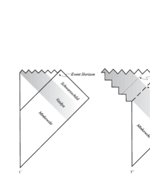
Depending on the distribution of matter in the null cloud, either black holes or naked singularities may develop as the classical final state of the collapse. For example, in the self similar model in which the mass is a linear function of the advanced null coordinate, , one finds that both outcomes described by the Penrose diagrams in figure 1 are possible, depending on whether (black hole) or (naked singularity) nsing .
When the collapse evolves toward a naked singularity, spatial hypersurfaces in the future of the initial singularity cross the Cauchy horizon and collide with the central singularity but, because no sensible boundary conditions can be specified on a singularity, the evolution in the future of the initial singularity is arbitrary. The Cosmic Censor Rp1 should come into play before the Cauchy horizon has a chance to form. It is of interest, therefore, to understand how the system behaves close to, but in the past of, the putative Cauchy horizon, where spatial hypersurfaces are well defined and the quantum evolution of the system may be studied.
Null shells classically collapse to form covered singularities, therefore, in order to examine such issues as the Cosmic Censor, mass distributions other than those representing shells should be considered. These require a quantization of a genuine field theory. The present paper is intended as a first step in this direction. The solution metric is written in Eddington-Finkelstein coordinates and the Kuchař transformation from ADM variables to Kuchař variables is established. The mass function is explicitly related to and of the metrics in (1), respectively (2).
The quantization program employed in this paper involves a gauge fixing and it is known that quantum theories resulting from different gauge fixings are not necessarily equivalent. It is, nevertheless, the best approach to the quantization of realistic and pressing problems such as gravitational collapse at this time. Our choice of configuration space coordinates presents several advantages: their physical meaning is transparent, we are able to give explicit transformations between the original ADM phase space and the new, and the constraints expressed in terms of the new phase space variables are linear. The last enables us to obtain solutions for null dust clouds of arbitrary mass distributions. The second implies that operators representing observables, if known in one system are easily constructed in the other, and the first makes our solutions easily interpretable in physical terms.
In section II we summarize the canonical formulation of the action in ADM variables. The null dust action appropriate to the models being considered is also analyzed in this section. In section III we explicitly perform a transformation of the phase-space to Kuchař variables ku1 . In section IV we apply Dirac’s quantization program to these models. Solutions to the constraints for collapsing and expanding clouds are presented and the matter distribution representing a single shell is examined as a special case. However, the phase-space admits non-trivial boundaries and this generally leads to complications in the quantization procedure. Our solutions are valid subject to the condition that a suitable measure can be found so that the replacement leads to self-adjoint operators. We conclude in section V with a discussion of the strengths and weaknesses of our approach, the issues that remain to be resolved (such as the question of observables and of the measure on the Hilbert space) as well as some suggestions for future directions.
II Canonical Formulation in ADM Variables
Consider the line element, on a spherically symmetric three dimensional Riemann surface, . It is completely characterized by two functions, and of the radial label coordinate
| (5) |
where is the solid angle. The angular coordinates play no role and will be integrated over. We take both and to be positive definite except, possibly, at the center. represents the physical radius of a shell labeled by on the surface. It behaves as a scalar under transformations of , whereas behaves as a scalar density. The corresponding four dimensional line element may be written in terms of two additional functions, the lapse, , and the shift, , as
| (6) |
In this spherically symmetric space-time, we will consider the Einstein-Dust system described by the action
| (7) | |||||
| (8) |
where is the scalar curvature. As is well known, the gravitational part of this action can be cast into the form
| (9) | |||||
| (11) |
with the momenta conjugate to and respectively given by
| (12) | |||||
| (13) |
and where the overdot and the prime refer respectively to partial derivatives with respect to the label time, , and coordinate, . The lapse, shift and phase-space variables are required to be continuous functions of the label coordinates. The boundary action, , is required to cancel unwanted boundary terms in the hypersurface action, ensuring that the hypersurface evolution is not frozen on the frontiers. It is determined after fall-off conditions appropriate to the models under consideration are specified. The super-Hamiltonian and super-momentum constraints are given by
| (14) | |||||
| (15) | |||||
| (17) |
We will assume that the matter distribution is such that at infinity Kuchař’s fall-off conditions ku1 are suitable and we will adopt them here. These conditions would be applicable, for example, in models in which the collapsing metric asymptotically approaches or is smoothly matched to an exterior Schwarzschild background at some boundary. They read
| (18) | |||||
| (19) | |||||
| (20) | |||||
| (21) | |||||
| (22) | |||||
| (23) |
and imply that the asymptotic regions are flat with the spatial hypersurfaces asymptotic to surfaces of constant Minkowski time. Again, as we require that Louko
| (24) | |||||
| (25) | |||||
| (26) | |||||
| (27) | |||||
| (28) | |||||
| (29) |
With these conditions, it is easy to see that the appropriate choice of surface action involves only the contribution,
| (30) |
at the boundary at infinity.
Let us now consider the null dust action in (8). We note first that the energy density, , plays the role of a Lagrange multiplier enforcing null dust, i.e., , and variation w.r.t. yields the standard dust stress tensor, . The canonical form of the null dust action in various forms has been studied by Kuchař and Bičák kuBi . In particular, for the action in the form given in (8) one may expand as a Pfaff form of six scalar fields, the three co-moving coordinates of the null dust particles, , and three scalars (velocities), ,
| (31) |
This representation is redundant because, by Pfaff’s theorem, only four scalars are required to describe an arbitrary covector in a four dimensional space. Suppose we require one of the scalars, say to be unity and drop the index from the associated co-moving coordinate, , then
| (32) |
Consider the independent variations,
| (33) | |||||
| (35) | |||||
| (37) | |||||
| (39) | |||||
| (41) | |||||
| (43) |
The conservation of the stress energy tensor in the last equation implies that
| (44) |
which says that the particles follow geodesic curves. Using the second equation above we find , implying affine parameterization. The third equation says that , i.e., all of the are constant along flow lines and none of them are time-like. And finally, multiplying the third equation by we find
| (45) |
saying that may be space-like or null. If the twist, , also vanishes, then is null, which would imply that , or , because the are taken to form a (linearly independent) cobasis.
Substituting the decomposition (32) into the dust action in (8), using (6) and integrating over the angular coordinates the action may be put in the form
| (46) |
where the momenta conjugate to are, respectively,
| (47) | |||||
| (49) |
and the constraints, and are
| (50) | |||||
| (52) |
Setting gives the final form of the dust Hamiltonian and momentum constraints
| (53) | |||||
| (55) |
where the positive (respectively negative) signs in the dust Hamiltonian density represent incoming (respectively outgoing) dust. In the spherically symmetric collapse we are considering, we take . Thus we have arrived at the canonical form of our theory, which we will write as
| (56) | |||||
| (58) | |||||
| (60) | |||||
| (61) | |||||
| (63) | |||||
| (65) |
where . In the following section we will show that the co-moving coordinate may be identified with the null coordinates according to for an expanding solution and for a collapsing one. and the dust Hamiltonian density is chosen to be always non-negative. When is non-vanishing the phase-space is made up of two disconnected sectors, labeled by . An initial data set with cannot evolve into a set with and we will assume from now on that .
III Canonical Transformation
The description of contracting and expanding clouds is seen to be related by time reversal. The two descriptions may be formally unified in the following way. Introduce a null coordinate , which can be the “advanced” time or the “retarded” time, satisfying only the requirement that increases toward the future. If (primes denote differentiation w.r.t. the ADM label coordinate ) then it represents the retarded coordinate, , and if, on the contrary, , it represents the advanced coordinate, . Let us write both solutions in terms of a parameter that represents the behavior of the matter (whether it is expanding or collapsing)
| (66) |
The metric (66) is appropriate for either expansion or contraction of the dust cloud depending on whether is or . is the same as appears in (65), as we argue below. The null coordinate, , whose spatial direction is opposite to is obtained by integrating
| (67) |
where is an integrating factor. This coordinate must also be always increasing toward the future.
The hypersurfaces (5) from which (6) is constructed must be embedded in the space-time described by the metric (66). Substituting the foliation and in (66) gives the density and the lapse and shift functions, and , as
| (68) | |||||
| (69) | |||||
| (70) |
where we have set . These relations can be used to determine,
| (71) | |||||
| (72) |
where we have chosen the sign of the square root so that is positive. Inserting these expressions for and in the expression (13) for , we find
| (73) |
which, when substituted into the expression for in (70), gives
| (74) |
or, equivalently, the mass function in terms of the canonical data
| (75) |
By directly taking Poisson brackets, the momentum conjugate to can now be shown to be simply
| (76) |
Kuchařku1 proposed that should form a canonical chart whose coordinates are spatial scalars, whose momenta are scalar densities and which is such that generates Diff R. This means that
| (77) |
Substituting the expressions derived for and into the above constraint one arrives at
| (78) |
where . One can then show that the transformation,
| (79) |
is canonical, and generated by
| (80) |
By computing the difference between the old and the new Liouville forms and using the fall off conditions in (23) and (29), one can show that the transformation has introduced no fresh boundary terms.
There are (infinite) boundary terms at the horizon, when . It can be shown, however, that the contribution from the interior and the exterior cancel each other. There will also be contributions at the boundary between the interior of the star and its exterior or more generally at any frontier between two regions described by mass functions with different derivatives. Again, if the mass function is continuous across the boundary and regions are consistently matched by equating both the first and second fundamental forms, then the contribution from one side will cancel the contribution from the other.
Before rearranging the action, we will consider the coordinates for the collapsing Vaidya null congruence. Returning to the metric in (66) with we find that the incoming null congruence is given by , and The coordinates , and are co-moving. Let us form the basis
| (81) | |||||
| (82) | |||||
| (83) |
It is easily shown that is an affine parameter and the covariant components of the velocity are , whose decomposition in the co-basis yields . Similarly treating the outgoing null congruence shows that the affine parameter is and that is to be identified with . Both cases may be treated simultaneously by letting , and . This identification shows that the used in the section is identical to that used in the previous section.
Note also that taking the spatial derivative of in (75), yields
| (84) |
This may be used to write the action in (8) as
| (85) |
with
| (86) | |||||
| (88) | |||||
| (90) |
The surface term contains the mass at spatial infinity and may be re-expressed in a more convenient form. Use the fall-off conditions (23) at infinity and the expression for in (72) to write and
| (91) |
Then define by
| (92) |
i.e., and is clearly the mass at infinity. The one form
| (93) |
can now be written as
| (96) | |||||
where is an exact form. The second term in the expression for continues to be inconvenient, but may be cast into a more appropriate form using the identity ku1
| (97) |
Integrating from to , the left hand side of the above equation vanishes identically and one finds
| (100) | |||||
so that can be cast into the form
| (101) |
where we have defined
| (102) | |||
| (103) | |||
| (104) |
Eliminating a total time derivative turns the action in (85) into
| (105) |
where
| (106) | |||||
| (108) |
Furthermore, it follows from (73) that
| (109) |
The constraints, , can be further simplified by using to eliminate from the Hamiltonian constraint. This gives
| (110) |
Consider the first of the two factors above. Using (109) to substitute for , we find
| (111) |
where is the integrating factor introduced in the previous section. But because it is a null coordinate and is required to increase in time, therefore,
| (112) |
is equivalent to the Hamiltonian constraint, . Inserting this into either of the two constraints then gives .
The configuration space is made of the set of variables , whose physical significance is transparent. This is an advantage of Kuchař variables. is a null coordinate, is the area radius of a point labeled , is the energy density of the collapsing cloud and is the mass measured at spatial infinity. is a constant of the motion and may be viewed as part of the initial data. Our gravity-matter system may be re-written as
| (113) |
The canonical action (113) can be a starting point for Dirac quantization. The physical meaning of all the configuration space coordinates is clear: and locate the hypersurface and (along with ) determines the matter distribution.
IV Quantization
The configuration space consists of two disconnected components, for expanding null matter it is spanned by the set and for collapsing matter by the set . In each case the phase-space has non-trivial boundaries,
| (114) | |||||
| (116) |
The last is due to the fact that describes the central singularity, i.e., the final singularity for the collapsing solution and the initial singularity for expanding one. In Dirac’s approach, when the phase-space admits trivial boundaries, the canonical momenta , are raised to operator status,
| (117) |
and the constraints are considered as operator restrictions on the state functional. When the boundaries are non-trivial, as is the case in (116), this naïve exchange of momenta for functional derivatives in (117) may lead to operators that are not self-adjoint isham , but we will assume here that a suitable measure on the Hilbert space can be found, with respect to which the above replacement leads indeed to self-adjoint operators. Subject to this caveat, the state-functional obeys
| (118) | |||||
| (120) |
The last constraint is solved by any functional that is a spatial scalar. Consider a solution of this constraint that is of the form
| (121) |
where is a constant depending only on and , and is an arbitrary complex valued function of its arguments (and not their derivatives) that is to be evaluated so that satisfies the other constraints. The wave-functional in (121) is evidently a spatial scalar because is a spatial density and is a spatial scalar. It is therefore a solution of the constraint providing that has no explicit dependence on .
The solution, which agrees with all the constraints considered as operator restrictions on the state functional, is given by
| (122) |
where is a “tortoise”-like coordinate defined by
| (123) |
It is not, of course, the tortoise coordinate except in a Schwarzschild region when is constant.
The parameter represents the direction of the flow, being for outgoing null matter and for incoming matter. The combination represents the affine parameter, . Re-expressing the wave-functional in (121) to make the dependence on the affine parameter explicit, we find
| (124) |
where .
For , and , the functionals are of the form
| (125) |
and describe collapsing null matter. Likewise, for , and , the functionals
| (126) |
describe expanding null matter.
A given classical collapse problem is specified by a choice of mass function, , which determines an initial energy distribution, thus a collapse “model”. As an example, we shall consider the function,
| (127) |
where is the Heaviside unit step-function and is constant. The matter energy vanishes when and is when . The mass function evidently makes sense only as a thin shell that is collapsing toward the center and we must have (). Calling the corresponding mass at spatial infinity , we find the energy density by differentiating w.r.t. the ADM label coordinate, ,
| (128) | |||||
| (130) |
where is the solution of . Likewise, a thin shell that expands out of the center is represented by the mass function
| (131) |
for (). The energy density is
| (132) | |||||
| (134) |
where is the solution of . The energy density is always positive and in either case we find
| (135) |
The shell trajectories, are different in the two cases, being in the first and in the second. Using these expressions, let us relate the constraints in (65) to the constraints that have been used by others to describe thin shells. The dust Hamiltonian and momentum density turn out to be ()
| (136) | |||||
| (138) |
where we have defined and therefore . These expressions were used as a starting point in Louko ; haj1 ; haj2 . The gravitational contributions to the constraints are, of course, the same.
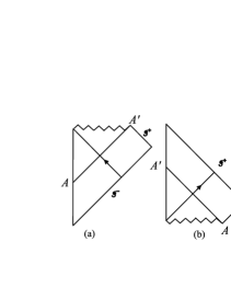
The corresponding classical solutions are represented in the Penrose diagram of figure 2, where represents the event horizon in (a) and the Cauchy horizon in (b).
Inserting (135) into (125) and (126) one finds that the quantum mechanics of a single collapsing shell is defined on the reduced configuration space and described by the wave-function
| (139) |
whereas, for an outgoing shell the reduced configuration space is and the wave-function
| (140) |
where as given by (123) is, in this case, the usual tortoise coordinate.
V Discussion
In this paper we have examined the collapse and expansion of a null dust cloud of arbitrary mass distribution and shown that there exists a canonical transformation that brings the corresponding Vaidya system to the Kuchař form, in which the dynamics is expressed in terms of embedding variables whose physical meaning is transparent. Written in terms of these variables, the constraints take on a simple form.
The physical content of the solution wave-functionals discussed in the previous section is given by the expectation values of observables. These are, for example, the geometric invariants and matter invariants (such as curvature scalars and trace of the stress energy tensor) and in general any function of the phase-space variables, old or new, that weakly commutes with the constraints. They must be written as operators on the Hilbert space, but there are two associated difficulties. Firstly, because they are generally non-linear, there will be operator ordering ambiguities. Secondly, one must ensure that they are self-adjoint with respect to the chosen measure. However, as our transformation between the spaces is explicit, knowing these functions in one system is equivalent to knowing them in the other. It should be noted that a complete set of Dirac observables has been constructed in the case of a single shell haj1 where a single degree of freedom is present. For the general case, this issue is quite complicated and will be discussed in the future.
Subject to the condition that suitable boundary conditions or a suitable inner product can be found so that (117) leads to self-adjoint operators, we have found solution wave-functionals for arbitrary mass distributions in each sector (collapse and expansion) independently (as mentioned in the introduction, solutions with non-trivial mass distributions are essential for the description of issues as naked singularities and the Cosmic Censor). These sectors are disjoint, separated by the central singularity (at ). However, if the solutions are viewed as describing the evolution, in the affine parameter , of a collapsing matter cloud beginning on , they seem to suggest that it should be possible to define the wave-functional over the entire interval by extending the range of to include the center. Yet, for any matter distribution, the solution space-time in (66) admits a strong curvature singularity at the origin, so the classical dynamics cannot be extended even to it. Any attempt to continue the quantum dynamics through the origin must therefore ensure that at least the expectation values of the observables in the consequent quantum theory are well behaved there. Thus the central singularity would be made harmless by the quantum theory. It can be so if, for example, the wave-functional were to vanish there. In this way the matter would collapse and re-expand through the (benign) center in one continuous history, the solutions being given by (125) for and (126) for . This has been proposed for a single shell by Hájíček and Kiefer haj1 ; haj1a ; haj2 , who merged the two solutions into one bouncing solution. Their bounce was obtained by working in double-null coordinates and employing group quantization techniques (see haj1 and haj3 ) to the problem. Group quantization is beautifully adapted to the quantization of systems with non-trivial boundary restrictions such as those in (116) on the phase space, but it’s application to problems with more than a few number of degrees of freedom and in particular to the collapse of general matter distributions, being dependent on the construction of a complete set of observables, remains a topic for future investigation.
The Eddington-Finkelstein coordinates we have employed in this paper present several advantages over the double null system in regard to the problem of collapse or re-expansion of arbitrary matter distributions. The new variables have a clear physical and geometrical meaning. This is useful when comparing the quantum behavior with the classical. Our transformations are explicit, which means that operators and, in particular, observables that are known in one coordinate system can be expressed in the other. The matter-gravity constraints in the new phase space are linear for all matter distributions. This simplification, achieved on the classical level, has allowed us to obtain exact solution wave-functionals describing the respective physical processes.
VI Acknowledgements
We acknowledge the partial support of FCT, Portugal, under contract number POCTI/32694/FIS/2000. L.W. was supported in part by the Department of Energy, USA, under contract Number DOE-FG02-84ER40153.
References
- (1) S. W. Hawking, Commun. Math. Phys. 43 (1975) 199.
- (2) J. D. Bekenstein, Phys. Lett. B481 (2000) 339; J. D. Bekenstein and A. Mayo, Phys, Phys. Rev. D61 (2000) 024022; S. Hod, Phys. Rev. D61, 024023 (2000); J. D. Bekenstein and M. Schiffer, Phys. Rev. D58 (1998) 064014; J. D. Bekenstein, Phys. Lett. B360 (1995) 7; ibid Phys. Rev. Lett. 70 (1993) 3680; ibid Phys. Rev. D9 (1974); ibid Phys. Rev. D7 (1973) 2333; ibid, Ph. D. Thesis, Princeton University, April 1972; ibid, Lett. Nuovo Cimento 4 (1972) 737.
- (3) K. V. Krasnov, Gen. Rel. Grav. 30 (1998) 53; A. Ashtekar, J. Baez, A. Corichi, K Krasnov, Phys. Rev. Letts. 80 (1998) 904; A. Ashtekar, J.Lewandowski, Class. Quant. Grav. 14 (1997) A55; H. A. Kastrup, Phys. Lett. B385 (1996) 75; ibid Phys. Letts. B413 (1997) 267; ibid Phys. Letts. B419 (1998) 40.
- (4) A. W. Peet, Class. Quant. Grav. 15 (1998) 3291; K. Sfetsos, K. Skenderis, Nucl. Phys. B517 (1998) 179; A. Strominger and C. Vafa, Phys. Lett. B379 (1996) 99; C. O. Lousto, Phys. Rev. D51 (1995) 1733; M. Maggiore, Nucl. Phys. B429 (1994) 205; Ya. I. Kogan, JETP Lett. 44 (1986) 267; A. Strominger, JHEP 9802 (1998) 009; J.M. Maldacena and A. Strominger, JHEP 9802 (1998) 014; J.M. Maldacena, A. Strominger and E. Witten, JHEP 9712 (1997) 002; G. Horowitz, D. Lowe and J.M. Maldacena, Phys. Rev. Lett. 77 (1996) 430-433.
- (5) J. Mäkelä, P. Repo, M. Luomajoki and J. Piilonen, Phys. Rev. D64 (2001) 024018; Cenalo Vaz and Louis Witten, Phys. Rev. D64 (2001) 084005; C. Kiefer and J. Louko, Annalen Phys. 8 (1999) 67; C. Kiefer, Nucl. Phys. B Proc. Suppl 57 (1997) 173; T. Brotz and C. Kiefer, Phys. Rev. D55 (1997) 2186; J. Louko and B.F. Whiting, Phys. Rev. D51 (1995) 5583; J. Louko, S. Winters-Hilt, Phys. Rev. D54 (1996) 2647; F. Larsen and F. Wilczek, Phys. Letts. B375 (1996) 37; J. Louko and J. Mäkelä, Phys. Rev. D54 (1996) 4982; P. Kraus and F. Wilczek, Nucl. Phys. B437 (1995) 231; F. Larsen and F. Wilczek, Annals Phys. 243 (1995) 280.
- (6) R. Penrose, Riv. Nuovo Cimento 1 (1969) 252; in General Relativity, An Einstein Centenary Survey, ed. S. W. Hawking and W. Israel, Cambridge Univ. Press, Cambridge, London (1979) 581.
- (7) see, for example, P. S. Joshi, Global Aspects in Gravitation and Cosmology, Clarendon Press, Oxford, (1993).
- (8) T.P. Singh and Cenalo Vaz, Phys. Rev. D61 (2000) 124005; T.P. Singh and Cenalo Vaz, Phys. Letts. B481 (2000) 74; S. Barve, T.P. Singh, Cenalo Vaz and Louis Witten, Nucl. Phys. B532 (1998) 361; S. Barve, T.P. Singh, Cenalo Vaz and Louis Witten, Phys. Rev. D58 (1998) 104018; S. Barve, T.P. Singh and Cenalo Vaz, Phys. Rev. D62 (2000) 084021; T. Harada, H. Iguchi and K. Nakao, Phys. Rev. D61, 101502 (2000); T. Harada, H. Iguchi and K. Nakao, Phys. Rev. D62, 084037 (2000); Cenalo Vaz and Louis Witten, Phys. Lett. B442 (1998) 90.
- (9) T. Harada, H. Iguchi, K. Nakao, T.P. Singh, T. Tanaka and Cenalo Vaz, Phys. Rev. D64 (2001) 041501.
- (10) P.C. Vaidya, Proc. Indian. Acad. Sci. A33, 264.
- (11) W. A. Hiscock, L. G. Williams and D. M. Eardley (1982) Phys. Rev. D26 751; Y. Kuroda (1984) Prog. Theor. Phys. 72 63; A. Papapetrou (1985) in A Random Walk in General Relativity, Eds. N. Dadhich, J. K. Rao, J. V. Narlikar and C. V. Vishveshwara (Wiley Eastern, New Delhi); G. P. Hollier (1986) Class. Quantum Grav. 3 L111; W. Israel (1986) Can. Jour. Phys. 64 120; K. Rajagopal and K. Lake (1987) Phys. Rev. D35 1531; I. H Dwivedi and P. S. Joshi (1989) Class. Quantum Grav. 6 1599; (1991) Class. Quantum Grav. 8 1339; P. S. Joshi and I. H. Dwivedi (1992) Gen. Rel. Gravn. 24 129; J. Lemos (1992) Phys. Rev. Lett. 68 1447.
- (12) K. V. Kuchař, Phys. Rev. D50 (1994) 3961.
- (13) C.J. Isham in “Relativity, groups and topology II”, ed. B.S. deWitt and R. Stora, Elsevier, Amsterdam, (1984).
- (14) J. Louko, B. Whiting and J. Friedman, Phys. Rev. D57 (1998) 2279.
- (15) J. Bičák and K.V. Kuchař, Phys.Rev. D56 (1997) 4878.
- (16) P. Hájíček, Nucl. Phys. B603 (2001) 555-577.
- (17) P. Hájíček and C. Kiefer, gr-qc/0107102.
- (18) P. Hájíček and C. Kiefer, Nucl. Phys. B603 (2001) 531-554.
- (19) P. Hájíček, J. Math. Phys. 36 (1995) 4612; P. Hájíček, A Iguchi and J. Tolar, J. Math. Phys. 36 (1995) 4639.