PARAMETRIC GRAVITY WAVE DETECTOR

Since 1978 superconducting coupled cavities have been proposed as a sensitive detector of gravitational waves. The interaction of the gravitational wave with the cavity walls, and the resulting motion, induces the transition of some energy from an initially excited cavity mode to an empty one. The energy transfer is maximum when the frequency of the wave is equal to the frequency difference of the two cavity modes. In 1984 Reece, Reiner and Melissinos built a detector of the type proposed, and used it as a transducer of harmonic mechanical motion, achieving a sensitivity to fractional deformations of the order $\delta x/x\approx 10^{-18}$. In this paper the working principles of the detector are discussed and the last experimental results summarized. New ideas for the development of a realistic gravitational waves detector are considered; the outline of a possible detector design and its expected sensitivity are also shown.

1 Introduction

In this paper we shall discuss the mechanism of the interaction of a gravitational wave with a detector based on two coupled electromagnetic cavities. In previous works this issue was discussed using the concept of a dielectric tensor associated with the gravitational wave.$\!{}^{{\bf?}}$ The interaction was analyzed in the reference frame where the resonator walls were at rest even in presence of a gravitational perturbation. Here we shall analyze the interaction in the proper reference frame attached to the detector and we shall therefore consider both the coupling between the wave and the mechanical structure of the detector and the perturbation induced on the field stored inside the resonator due to the time–varying boundary conditions.

The proposed detector exploits the energy transfer induced by the gravitational wave between two levels of an electromagnetic resonator, whose frequencies $\omega_{1}$ and $\omega_{2}$ are both much larger than the characteristic angular frequency $\Omega$ of the g.w. and satisfy the resonance condition $\omega_{2}-\omega_{1}=\Omega$. The interaction between the g.w. and the detector is characterized by a transfer of energy and of angular momentum. Since the elicity of the g.w. (i.e. the angular momentum along the direction of propagation) is 2, it can induce a transition between the two levels provided their angular momenta differ by 2; this can be achieved by putting the two cavities at right angle or by a suitable polarization of the electromagnetic field axis inside the resonator. In the scheme suggested by Bernard et al. the two levels are obtained by coupling two identical high frequency cavities.$\!{}^{{\bf?},{\bf?}}$ The angular frequency $\omega_{1}$ is the frequency of the level symmetrical in the fields of the two cavities, and $\omega_{2}$ is that of the antisymmetrical one. The frequency difference between the symmetric and the antisymmetric level is determined by the coupling and can be adjusted by a careful resonator design. Since the detector sensitivity is proportional to the square of the resonator quality factor, superconducting cavities must be used for maximum sensitivity.

The power transfer between the levels of a resonator made up of two pill-box cavities, mounted end-to-end and coupled by a small circular aperture in their common end wall, was checked in a series of experiments by Melissinos et al., where the perturbation of the resonator volume was induced by a piezoelectric crystal.$\!{}^{{\bf?},{\bf?}}$

Recently the experiment was repeated by our group with an improved experimental set-up;$\!{}^{{\bf?}}$ we obtained an order of magnitude sensitivity to fractional deformations of the resonator length as small as $\delta\ell/\ell\approx 10^{-20}$ Hz^-1/2.

In this paper we shall discuss the detector’s working principles and briefly review the last experimental results obtained by our group on the first prototype. Finally a possible detector design, based on two coupled spherical cavities, is discussed and its expected sensitivity is shown.

2 Fundamental principles

When the resonator’s boundary is deformed by an external force the local displacement vector, $\vec{u}(\vec{r},t)$, can be expressed as a superposition of the mechanical undamped normal modes $\{\vec{\xi}_{\alpha}(\vec{r})\}$: $\vec{u}(\vec{r},t)=\sum_{\alpha}q_{\alpha}(t)\vec{\xi}_{\alpha}(\vec{r})$. $q_{\alpha}(t)$ is the generalized coordinate of the $\alpha_{th}$ mode, obeying the dynamical equation of motion:

$$\ddot{q}_{\alpha}(t)+\frac{\omega_{\alpha}}{Q_{\alpha}}\,\dot{q}_{\alpha}(t)+\omega_{\alpha}^{2}q_{\alpha}(t)=\frac{f_{\alpha}(t)}{M_{\alpha}}$$ (1)

and the modes are normalized according to the relation

$$\int_{Vol}\rho(\vec{x})\vec{\xi}_{\alpha}(\vec{x})\cdot\vec{\xi}_{\beta}(\vec{x})\,dV=M_{\alpha}\delta_{\alpha\beta}$$ (2)

being $\rho(\vec{x})$ the mass density and $M_{\alpha}$ the reduced mass of the $\alpha^{th}$ mode. For a homogeneous system $M_{\alpha}\equiv M$, where $M$ is the mass of the system.

In eq. 1 an empirical damping term, proportional to the velocity, has been included.

$f_{\alpha}(t)$ is the generalized force, given by

$$f_{\alpha}(t)=\int_{Vol}\vec{f}(\vec{r},t)\cdot\vec{\xi}_{\alpha}(\vec{r})\,dV$$ (3)

where $\vec{f}(\vec{r},t)$ is the external force density acting on the system.

For a plane g.w travelling along the $z$ axis the force density, in the proper reference frame attached to the detector, has the form:

$$\vec{f}(\vec{x},t)=-\frac{1}{2}\rho(\vec{x})\left(\ddot{h}^{1}_{\,1}x+\ddot{h}^{1}_{\,2}y,\ddot{h}^{1}_{\,2}x-\ddot{h}^{1}_{\,1}y,0\right)$$ (4)

where $h^{i}_{j}(t)$, is the adimensional amplitude of the wave, and $h^{1}_{\,1}=-h^{2}_{\,2}$, $h^{1}_{\,2}=h^{2}_{\,1}$.

To study the mechanism of the energy transfer between the two levels of an electromagnetic resonator perturbed by a gravitational wave we shall make use of the fact that the electromagnetic field inside the resonator can be expanded over the fields of the normalized, orthogonal normal modes $\{\vec{E}_{n}(\vec{r})\}$ and $\{\vec{H}_{n}(\vec{r})\}$: $\!{}^{{\bf?}}$

$$\vec{E}=\sum_{n}\left(\int_{V}\vec{E}\cdot\vec{E}_{n}\,dV\right)\vec{E}_{n}\;;\;\vec{H}=\sum_{n}\left(\int_{V}\vec{H}\cdot\vec{H}_{n}\,dV\right)\vec{E}_{n}$$ (5)

For simplicity we shall assume that in the frequency range of interest only two e.m. modes give a significant contribution ($n=1,2$), and that the external force couples strongly only to one mechanical mode ($\alpha=m$). If we now introduce a perturbation of the resonator boundary and assume that the perturbation is small i.e. that we can still expand the fields inside the perturbed volume over the normal modes of the unperturbed resonator, we obtain the following set of equations for the magnetic field expansion coefficients:

$$\ddot{\cal H}_{1}(t)+\frac{\omega_{1}}{\mathcal{Q}_{1}}\dot{\cal H}_{2}(t)+\omega_{1}^{2}{\cal H}_{1}(t)=-\omega_{1}q_{m}(t)\left(C^{m}_{11}{\cal H}_{1}(t)+C^{m}_{12}{\cal H}_{2}(t)\right)$$ (6)

$$\ddot{\cal H}_{2}(t)+\frac{\omega_{2}}{\mathcal{Q}_{2}}\dot{\cal H}_{2}(t)+\omega_{2}^{2}{\cal H}_{2}(t)=-\omega_{2}q_{m}(t)\left(C^{m}_{21}{\cal H}_{1}(t)+C^{m}_{22}{\cal H}_{2}(t)\right)$$ (7)

$$\ddot{q}_{m}(t)+\frac{\omega_{m}}{Q_{m}}\,\dot{q}_{m}(t)+\omega_{m}^{2}q_{m}(t)=\frac{f_{m}(t)}{M}+\frac{f_{m}^{ba}(t)}{M}$$ (8)

where we have defined the time–dependent expansion coefficients as ${\cal E}_{i}(t)\equiv\sqrt{\epsilon_{0}}\int_{V}\vec{E}\cdot\vec{E}_{i}\,dV$ , ${\cal H}_{i}(t)\equiv\sqrt{\mu_{0}}\int_{V}\vec{H}\cdot\vec{H}_{i}\,dV$ and the coupling coefficients as:

$$C^{m}_{ij}\equiv\int_{{S}}(\omega_{i}\vec{H}_{i}\cdot\vec{H}_{j}-\omega_{j}\vec{E}_{i}\cdot\vec{E}_{j})\,\vec{\xi}_{m}\cdot d\vec{S}$$ (9)

The integral in eq. 9 is made on the unperturbed surface of the resonator.

The electromagnetic quality factor ${\cal Q}_{n}=G_{n}/R_{s}$, takes into account the dissipation arising from the finite conductivity of the walls. $R_{s}$ is the material–dependent surface resistance of the walls, and the geometric factor $G_{n}$ of the $n_{th}$ e.m. mode is given by:

$$G_{n}=\omega_{n}\mu_{0}\frac{\int_{V}H_{n}^{2}\,dV}{\int_{S}H_{n}^{2}\,dS}$$ (10)

In the following we shall assume $\mathcal{Q}_{1}\approx\mathcal{Q}_{2}\equiv\mathcal{Q}$.

The term $f_{m}^{ba}$, in the r.h.s. of eq. 8, describes the deformation of the walls induced by the stored e.m. fields, i.e. a back–action effect of the e.m. field on the detector’s boundary: it is well known that in a resonant cavity the stored magnetic field interacts with the rf wall current, resulting in a Lorenz force which causes a deformation of the cavity shape.$\!{}^{{\bf?},{\bf?}}$ The radiation pressure is given by:

$$P_{L}(\vec{r},t)=\frac{1}{2}\left(\mu_{0}\vec{H}(\vec{r},t)^{2}-\epsilon_{0}\vec{E}(\vec{r},t)^{2}\right)$$ (11)

Expanding again the fields $\vec{E}$ and $\vec{H}$ in terms of the normal modes (eq. 5) we get:

$$P_{L}(\vec{r},t)=$$ (12)

$$\frac{1}{2}\left(\mathcal{H}_{1}(t)^{2}\vec{H}_{1}(\vec{r})^{2}+\mathcal{H}_{2}(t)^{2}\vec{H}_{2}(\vec{r})^{2}+2\,\mathcal{H}_{1}(t)\mathcal{H}_{2}(t)\vec{H}_{1}(\vec{r})\cdot\vec{H}_{2}(\vec{r})\right)-$$

$$\frac{1}{2}\left(\mathcal{E}_{1}(t)^{2}\vec{E}_{1}(\vec{r})^{2}+\mathcal{E}_{2}(t)^{2}\vec{E}_{2}(\vec{r})^{2}+2\,\mathcal{E}_{1}(t)\mathcal{E}_{2}(t)\vec{E}_{1}(\vec{r})\cdot\vec{E}_{2}(\vec{r})\right)$$

Since $\mathcal{H}_{1}(t)\sim\exp(j\omega_{1}t)$, $\mathcal{H}_{2}(t)\sim\exp(j\omega_{2}t)$, $\mathcal{E}_{1}(t)\sim\exp(j\omega_{1}t)$ and $\mathcal{E}_{2}(t)\sim\exp(j\omega_{2}t)$ only the cross-product terms will give a significant contribution at the resonance frequency $\Omega=\omega_{2}-\omega_{1}$. The other, rapidly oscillating terms, will just give an average deformation of the detector’s walls, determining a static frequency shift of the resonant modes, which can easily be compensated by an external tuning device.$\!{}^{{\bf?}}$

The generalized back–action force (cfr. eqs. 3 and 8), acting on the $m_{th}$ mechanical mode of the structure, will be given by:

$$f^{ba}_{m}=$$ (13)

$$\frac{1}{2}\mathcal{H}_{1}(t)\mathcal{H}_{2}(t)\int_{S}\left(\vec{H}_{1}\cdot\vec{H}_{2}\right)\,\vec{\xi}_{m}\cdot d\vec{S}-\frac{1}{2}\mathcal{E}_{1}(t)\mathcal{E}_{2}(t)\int_{S}\left(\vec{E}_{1}\cdot\vec{E}_{2}\right)\,\vec{\xi}_{m}\cdot d\vec{S}\equiv$$

$$\frac{1}{2}\mathcal{A}^{m}_{21}\,\mathcal{H}_{2}(t)\mathcal{H}_{1}(t)-\frac{1}{2}\mathcal{B}^{m}_{21}\,\mathcal{E}_{2}(t)\mathcal{E}_{1}(t)$$

where we have introduced the coefficients $\mathcal{A}^{m}_{21}\equiv\int_{S}\left(\vec{H}_{1}\cdot\vec{H}_{2}\right)\,\vec{\xi}_{m}\cdot d\vec{S}$ and $\mathcal{B}^{m}_{21}\equiv\int_{S}\left(\vec{E}_{1}\cdot\vec{E}_{2}\right)\,\vec{\xi}_{m}\cdot d\vec{S}$.

The analysis of the system of differential equations 6–8 can be simplified if we neglect the small perturbation on the initially excited e.m. mode (say mode 1), just taking into account the effects on the initially empty mode. Furthermore we shall consider the coupling between two TE modes of a resonator: for these modes we have vanishing electric field on the resonator surface and, as can readily be calculated, $C^{m}_{22}=0$ and $\mathcal{A}^{m}_{21}\approx C^{m}_{21}/\omega_{2}$.

With this assumptions we can recast the coupled system of equations in the following form:

$$\ddot{\cal H}_{2}(t)+\frac{\omega_{2}}{\mathcal{Q}}\dot{\cal H}_{2}(t)+\omega_{2}^{2}{\cal H}_{2}(t)=-\omega_{2}q_{m}(t)C^{m}_{21}{\cal H}_{1}(t)$$ (14)

$$\ddot{q}_{m}(t)+\frac{\omega_{m}}{Q_{m}}\,\dot{q}_{m}(t)+\omega_{m}^{2}q_{m}(t)=\frac{f_{m}(t)}{M}+\frac{1}{2}\frac{C^{m}_{21}}{M\omega_{2}}\,{\cal H}_{2}(t){\cal H}_{1}(t)$$ (15)

The solution of quations 14–15 is straightforward when the back–action term is switched off in eq. 15 and if we assume ${\cal H}_{1}(t)=\Re{(A\exp(i\omega_{1}t))}$. In this case we have the following asymptotic solution (in the frequency domain):

$$q_{m}(\omega)=\frac{f_{m}(\omega)/M}{(-\omega^{2}+\omega_{m}^{2}+i\,\omega\omega_{m}/Q_{m})}$$ (16)

and

$${\cal H}_{2}(\omega)=$$ (17)

$$-\frac{1}{2}\frac{\omega_{2}AC^{m}_{21}}{-\omega^{2}+\omega_{2}^{2}+i\,\omega\omega_{2}/{\cal Q}}\,\frac{f_{m}(\omega-\omega_{1})/M}{-(\omega-\omega_{1})^{2}+\omega_{m}^{2}+i\,\omega_{m}(\omega-\omega_{1})/{Q_{m}}}+$$

$$-\frac{1}{2}\frac{\omega_{2}AC^{m}_{21}}{-\omega^{2}+\omega_{2}^{2}+i\,\omega\omega_{2}/{\cal Q}}\,\frac{f_{m}(\omega+\omega_{1})/M}{-(\omega+\omega_{1})^{2}+\omega_{m}^{2}+i\,\omega_{m}(\omega+\omega_{1})/{Q_{m}}}$$

The field amplitude will be maximum when $\omega\approx\omega_{2}$. If we design our detector so that $\omega_{2}-\omega_{1}=\omega_{m}$ we have:

$$\mathcal{H}_{2}(\omega_{2})\approx\frac{1}{2}AC^{m}_{21}\frac{f_{m}(\omega_{m})}{M}\frac{\mathcal{Q}Q_{m}}{\omega_{2}\omega_{m}^{2}}$$ (18)

Eq. 18 shows that the amplitude of field in the initially empty mode is proportional to the amplitude of the field in the excited mode $A$, and to the electromagnetic ($\mathcal{Q}$) and mechanic ($Q_{m}$) quality factor of the system.

A detailed dicussion of the derivation of equations 6–8 and of the noise sources affecting the performance of the detector will be given elsewhere.

3 Experimental results

Figure 1: Superconducting cavity mounted on the test cryostat.

The electromagnetic properties of a prototype detector, made up of two pill–box cavities, mounted end–to–end, and coupled trough an iris on the axis, were measured in a vertical cryostat after careful tuning of the two cells frequencies. In order to get maximum sensitivity we need to have two identical coupled e.m. resonators, or, in other words, a flat field distribution between the two cavities. The symmetric mode frequency was measured at 3.03 GHz and the mode separation was 1.38 MHz.

In order to suppress the noise coming from the symmetric mode at the detection frequency, the transmission detection scheme, with two magic–tees, was used, as described elsewhere.$\!{}^{{\bf?}}$

In figure 2 the signal from the $\Delta$ port of the output magic–tee is shown for an input power $P_{i}=1$ W and no adjustments made on the phase and amplitudes of the rf signal entering and leaving the cavity. The overall attenuation of the symmetric mode is $R\approx-48$ dB.

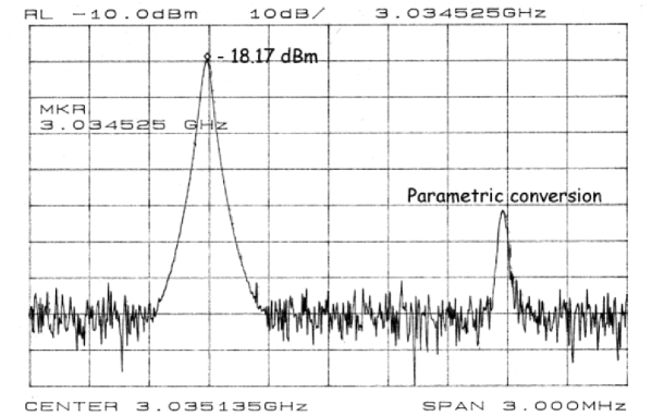
Figure 2: Transmission of the symmetric mode (no optimization) measured at the $\Delta$ port of the output magic–tee.

After balancing the arms of the two magic–tees in order to launch the symmetrical mode at the cavity input and to pick up the antisymmetrical one at the cavity output, with 1 W (30 dBm) of power at the $\Sigma$ port of the first magic–tee, $6.3\times 10^{-15}$ W (-112 dBm) were detected at the $\Delta$ port of the second one, giving an overall attenuation of the symmetric mode of $R\approx-140$ dB (see figure 3). At a detection frequency of $\Omega/2\pi\approx 1$ MHz the sensitivity of the system is quite independent from the value of $R$, because of the high cavity $\cal{Q}$. Nevertheless for lower frequencies, in a range $\Omega\leq 10$ kHz, where astrophysical sources of gravitational waves are expected to exist, this noise source can become dominant and the achieved rejection is fundamental in order to pursue the design of a working g.w. detector in the 1–10 kHz frequency range.

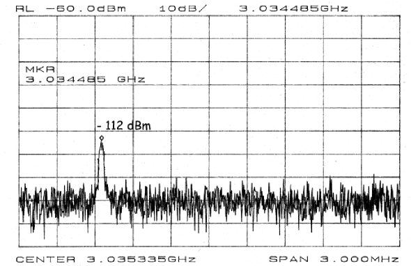
Figure 3: Transmission of the symmetric mode in the optimized system, measured at the $\Delta$ port of the output magic–tee. Measurement taken with 1 kHz resolution bandwidth.

The cavity loaded quality factor was $\mathcal{Q}_{L}=1\times 10^{9}$ at 1.8 K, and the energy stored in the cavity with 10 W input power was approximately 1.8 J (limited by the maximum power delivered by the rf amplifier), with both the input and output ports critically coupled ($\beta_{1}\approx\beta_{2}\approx 1$).

To excite the antisymmetric mode a piezoelectric crystal (Physik Instrument PIC 140, with longitudinal piezoelectric coefficient $\kappa_{\ell}=2\times 10^{-10}$ m/V) was fixed to one cavity wall. The driving signal to the crystal was provided by a synthesized oscillator with a power output in the range 2–20 mW (3–13 dBm). The oscillator output was further attenuated to reduce the voltage applied to the piezo by a series of fixed attenuators and a variable attenuator (10 dB step). The oscillator frequency was carefully tuned to maximize the energy transfer between the cavity modes.

The signal emerging from the $\Delta$ port of the output magic–tee was amplified by the LNA (48 dB gain) and fed into a spectrum analyzer. In figure 2 an example of the parametric conversion process is shown.

The minimum detected noise signal level at the antisymmetric mode frequency, with no excitation coming from the piezo, was $P_{out}(\omega_{2})=5\times 10^{-19}$ W in a bandwidth $\delta f=100$ Hz, giving a noise power spectral density ${\mathcal{P}}_{out}(\omega_{2})=5\times 10^{-21}$ W/Hz; the main contribution to this signal was the johnson noise of the rf amplifier used to amplify the signal picked from the $\Delta$ port of the output magic–tee.

Taking into account the input and output coupling coefficients the sensitivity if the system is given by $h_{min}\approx 3\times 10^{-20}\mathrm{(Hz)}^{-1/2}$

4 Future perspectives

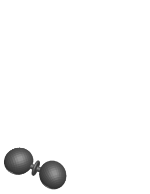
Figure 4: Artistic view of the coupled spherical cavities with the central tuning cell.

The second phase of the R&D program is focused on the development of a detector based on two spherical coupled cavities (see figure 4). In order to approach the interesting frequency range for g.w. detection, the mode splitting (i.e. the detection frequency) will be $\omega_{2}-\omega_{1}\approx 10$ kHz. The internal radius of the spherical cavity will be $r\approx 100$ mm, corresponding to a frequency of the TE₀₁₁ mode $\omega\approx 2$ GHz. The overall system mass and length will be $M\approx 5$ kg and $L\approx 0.8$ m. The choice of these frequencies for the resonator and mode splitting will be also useful in order to test the feasibility of a detector working at $\approx 200$ MHz and at a detection frequency of $\approx 1$ KHz.

A tuning cell, or a superconducting bellow, will be inserted in the coupling tube between the two cavities, allowing to tune the coupling strength (i.e. the detection frequency) in a narrow range around the design value.

The choice of spherical cells depends on several factors:

• From the point of view of the electromagnetic design the spherical cell has the highest geometrical factor, and so the highest quality factor, for a given surface resistance.

For the TE₀₁₁ mode of a sphere the geometric factor $G$ has a value $G\approx 850\,\Omega$, while for a standard elliptical accelerating cavity the TM₀₁₀ mode has a value of $G\approx 250\,\Omega$. Looking at the best reported values of quality factor of accelerating cavities, which typically are in the range $10^{10}-10^{11}$, we can extrapolate that the quality factor of the TE₀₁₁ mode of a spherical cavity can exceed $\mathcal{Q}\approx 10^{11}$.

• From the mechanical point of view it is well know that a sphere has the highest interaction cross-section with a g.w. and that only a few mechanical modes of the sphere do interact with a gravitational perturbation (the quadrupolar ones).$\!{}^{{\bf?}}$

The mechanical design is highly simplified if the spherical geometry is used since the deformation of the sphere is given by the superposition of just one or two normal modes of vibration and thus can be easily modeled. In fact the proposed detector acts essentially as a standard g.w. resonant bar detector: the gravitational perturbation interacts with the mechanical structure of the resonator, deforming it. The e.m. field stored inside the resonator is affected by the time–varying boundary conditions and a small quantity of energy is transferred from the initially excited e.m. mode to the initially empty one, provided the g.w. frequency equals the frequency difference of the two modes. A possible design of the detector makes use of both the mechanical resonance of the resonator structure, and the e.m. resonance. This can be accomplished if the detector is designed in order to have the mechanical mode frequency equal to the e.m. modes frequency difference $\omega_{m}=\omega_{2}-\omega_{1}$. In particular, for the detector designed to work in the 10 kHz frequency range, the two lowest quadrupolar modes frequency will be approximately at 4 and 17 kHz. The expected sensitivities of the detector for $\omega_{2}-\omega_{1}=4$ kHz and $\omega_{2}-\omega_{1}=10$ kHz are shown in figures 5 and 6. In the calculation of the above curves the brownian motion contribution to the detector noise as well as the noise coming from the detection electronics has been taken into account. Note that, also when $\omega_{2}-\omega_{1}\neq\omega_{m}$ (fig. 6) the sensitivity of the system is fairly good.

Figure 5: Calculated system sensitivity for a periodic source after 1 year integration time ($\omega_{m}=\omega_{2}-\omega_{1}=4$ kHz, $\mathcal{Q}=10^{11}$, $Q_{m}=5\times 10^{3}$, $T=1.8$ K).

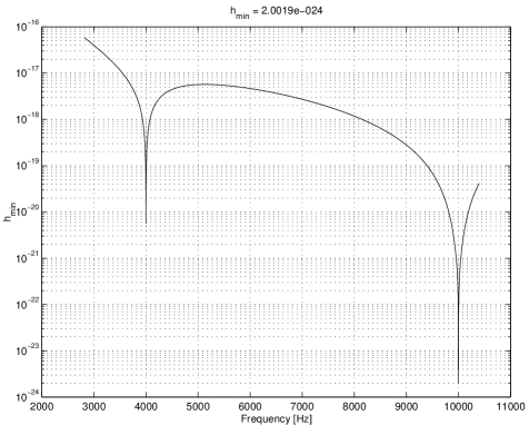
Figure 6: Calculated system sensitivity for a periodic source after 1 year integration time ($\omega_{m}=4$ kHz, $\omega_{2}-\omega_{1}=10$ kHz, $\mathcal{Q}=10^{11}$, $Q_{m}=5\times 10^{3}$, $T=1.8$ K).

• The spherical cells can be esily deformed in order to remove the unwanted e.m. modes degeneracy and to induce the field polarization suitable for g.w. detection.

The interaction between the stored e.m. field and the time-varying boundary conditions is not trivial and depends both on how the boundary is deformed by the external perturbation and on the spatial distribution of the fields inside the resonator. It has been calculated that the optimal field spatial distribution is with the field axis of the two cavities orthogonal to each other. Different spatial distributions (e.g. with the field axis along the resonators’ axis) give a smaller effect or no effect at all.

• The spherical shape can be easily used to investigate whether the niobium-on- copper technique could be useful for the detector final design.

The choice between bulk niobium or niobium–on–copper for the final detector design has not yet been made and is still under investigation. Both techniques present in principle advantages and drawbacks. A prototype of two coupled spherical cavities in bulk niobium will be built at CERN in 2002. A single cell, seamless, copper spherical cavity has been built at INFN-LNL by E. Palmieri and will be sputter coated at CERN.

5 Conclusions

A first prototype of the detector, made up of two pill-box cavities, mounted end-to- end, has been built and successfully tested. A detector based on two coupled spherical cavities is now being designed, and preliminar tests on nomal conducting prototypes are being made. The planned timeline is as follows:

• In 2002 a bulk niobium detector (two spherical cavities, $\omega=2$ GHz, $\Omega=10$ kHz, fixed coupling) will be built at CERN;

• In 2003 a variable coupling detector will be built and tested.

If experimental results will be encouraging, by the end of 2003 a proposal for the realization of a g.w. detector, based on superconducting rf cavities will be made.

References

References

- [1] F. Pegoraro and L.A. Radicati. Dielectric tensor and magnetic permeability in the weak field approximation of general relativity. Journal of Physics A, 13:2411–2421, 1980.
- [2] F. Pegoraro, L.A. Radicati, Ph. Bernard, and E. Picasso. Electromagnetic detector for gravitational waves. Physics Letters, 68A(2):165–168, 1978.
- [3] F. Pegoraro, E. Picasso, and L.A. Radicati. On the operation of a tunable electromagnetic detector for gravitational waves. Journal of Physics A, 11(10):1949–1962, 1978.
- [4] C.E. Reece, P.J. Reiner, and A.C. Melissinos. Observation of cm harmonic displacement using a 10 superconducting parametric converter. Physics Letters, 104A(6,7):341, 1984.
- [5] C.E. Reece, P.J. Reiner, and A.C. Melissinos. Parametric converters for detection of small harmonic displacements. Nuclear Instruments and Methods, A245:299–315, 1986.
- [6] Ph. Bernard, G. Gemme, R. Parodi, and E. Picasso. A detector of small harmonic displacements based on two coupled microwave cavities. Review of Scientific Instruments, 72(5):2428–2437, 2001. gr-qc/0103006.
- [7] J.C. Slater. Microwave Electronics. D. Van Nostrand Company, Inc., New York, 1950.
- [8] H. Padamsee, J. Knobloch, and T. Hays. Rf superconductivity for accelerators. John Wiley & Sons, New York, 1998.
- [9] J.A. Lobo. What can we learn about gw physics with an elatic spherical antenna? Physical Review D, 52:591, 1995.