TUW–01–31

Vers. 1.2

Virtual black hole phenomenology from $\boldsymbol{2d}$ dilaton theories

D. Grumiller

Institut für Theoretische Physik

Technische Universität Wien

Wiedner Hauptstr. 8–10, A-1040 Wien

Austria

Equipped with the tools of (spherically reduced) dilaton gravity in first order formulation and with the results for the lowest order $S$-matrix for $s$-wave gravitational scattering (P. Fischer, D. Grumiller, W. Kummer, and D. Vassilevich, Phys. Lett. B521 (2001) 357-363) new properties of the ensuing cross-section are discussed. We find $CPT$ invariance, despite of the non-local nature of our effective theory and discover pseudo-self-similarity in its kinematic sector.

After presenting the Carter-Penrose diagram for the corresponding virtual black hole geometry we encounter distributional contributions to its Ricci-scalar and a vanishing Einstein-Hilbert action for that configuration. Finally, a comparison is done between our (Minkowskian) virtual black hole and Hawking’s (Euclidean) virtual black hole bubbles.

PACS numbers: 04.60.Kz; 04.60.Gw; 11.10.Lm; 11.80.Et

1 Introduction

Ever since John Wheelers proposal of “space-time foam” [1] physicists have toyed with the idea of quantum induced topology fluctuations. This has culminated not only in the quite successful spin-foam models, which are considered as a serious candidate for quantum gravity (cf. e.g. [2]), but (among others) also in Hawking’s bubble approach of virtual black holes (VBH) [3]. What are the observational consequences of VBHs? There have been suggestions that VBHs might lead to loss of quantum coherence [4], violation of quantum mechanics [5], possibly affecting neutrino-oscillations [6], CPT-violation [7], non-standard Kaon-dynamics [8] etc.

In a recent work [9] we drew attention to a purely gravitational effect of VBHs, i.e. no other interactions were involved. We discussed gravitationally interacting massless scalars for the important special case of spherical symmetry in $d=4$ using the tools of first order dilaton gravity in $d=2$. After an exact (path) integration of the geometric variables (which had been performed elsewhere [10]) we encountered the VBH (our notion of VBHs differs from Hawking’s definition; but as we will point out it is justified to call our objects “virtual black holes”, so we stick to this name and apologize for eventual confusion caused by this difference). This is remarkable insofar as Hawking’s VBHs do not seem to be compatible with the special case of spherical symmetry because they can only be created in pairs [3]. The VBH we were describing exists even for that simple scenario. Using this VBH we were able to calculate the lowest order $S$-matrix for $s$-wave gravitational scattering. As suggested in [11] black holes played indeed an important role as intermediate states for the $S$-matrix.

After recalling briefly the main results of [9] (in section 2) we discuss in the present work new properties of the $S$-matrix for $s$-wave gravitational scattering and the corresponding VBH:

• By a simple calculation we observe (tree-level) $CPT$ invariance, which is remarkable insofar, as our effective action has been a non-local one and thus $CPT$-invariance is not granted by the $CPT$ theorem (section 3).

• We discuss the kinematic sector of the cross-section for (lowest order) gravitational $s$-wave scattering and observe as a new feature pseudo-self-similarity (section 4).

• Although the VBH geometry is a non-local entity we are able to present an easy interpretable Carter-Penrose diagram resembling a shock-wave geometry with evaporating shock. The Ricci-scalar of that geometry contains distributional contributions $\delta$ and $\delta^{\prime}$ and yields a vanishing Einstein-Hilbert action (section 5 and appendix A).

• Finally, we compare with Hawking’s VBHs and point out some parallels – the main difference is rooted in the Minkowskian signature we are using as opposed to Hawking’s Euclidean approach (section 6).

2 From first order gravity to the $\boldsymbol{S}$-matrix

We use the same notation as in [12, 10, 9, 13] and restrict our discussion again to spherically reduced gravity (SRG), i.e. $4d$ line elements of the form ($\alpha,\beta=0,1$)

$$ds^{2}=g_{\alpha\beta}dx^{\alpha}dx^{\beta}-X(x^{\alpha})d^{2}\Omega_{S^{2}},$$ (1)

using the signature $(+,-,-,-)$. The first order action

$$L_{\text{FO}}=-\frac{8\pi}{\kappa}\int_{M_{2}}{\big{[}}X^{+}(d-\omega)\wedge e^{-}+X^{-}(d+\omega)\wedge e^{+}+Xd\wedge\omega\\ -e^{-}\wedge e^{+}{\cal V}(X^{+}X^{-},X)+F(X)d\phi\wedge\ast d\phi{\big{]}}.$$ (2)

is (classically) equivalent to the spherically symmetric Einstein-massless-Klein-Gordon-model, i.e. it reproduces the spherically symmetric Einstein equations and the corresponding massless Klein-Gordon equation, provided the coupling function is chosen to be $F(X)=-\kappa X/2$ with $\kappa=8\pi G_{N}:=1$. Roughly speaking, it combines the advantages of a Hamiltonian formulation (“symplectic” structure, first order action) with the advantages of a Lagrangian formulation (manifest diffeomorphism invariance) [16].

These advantages, combined with a convenient choice of gauge, allow for an exact path integral quantization of the geometric part of (2) [17, 18]. However, the final matter-integration could only be performed perturbatively (supposing the scalar particles have a typical energy which is small compared to the Planck energy).

2.1 Minimal vs. nonminimal coupling

A comparison between the results for (in $d=2$) minimally coupled scalars (i.e. with $F(X)=$ const.) [12] and spherically reduced scalars shows not only quantitative but also essential qualitative changes [9]. Remarkably, these changes can be seen already at a rather fundamental level: the constraint algebra of the (first class) secondary constraints, $\{G_{i}(x),G_{j}(x^{\prime})\}=\delta(x-x^{\prime})C_{ij}{}^{k}(x)G_{k}(x)$, with $i=1,2,3$ and $\{\bullet,\bullet\}$ being the Poisson bracket. The nonvanishing structure functions are given by [10]
$\displaystyle C_{12}{}^{2}=-1,$ $\displaystyle C_{13}{}^{3}=1,$ $\displaystyle C_{23}{}^{1}=-\frac{\partial{\cal{V}}}{\partial X}+\frac{F^{\prime}(X)}{(e)F(X)}{\cal{L}}^{(m)},$ $\displaystyle C_{23}{}^{2}=-\frac{\partial{\cal{V}}}{\partial X^{+}},$ $\displaystyle C_{23}{}^{3}=-\frac{\partial{\cal{V}}}{\partial X^{-}}.$ (3)
Without matter or in the simple case of $F(X)=$const. the exceptional term in (3) proportional to $dF/dX$ vanishes. We call this term exceptional because as opposed to all other terms in (3) it is not only a function of the dilaton $X$ and the auxiliary fields $X^{\pm}$, but it also depends on the scalar field, its momentum and the vielbein. This qualitative change of the constraint algebra has far-reaching technical consequences: the system of partial differential equations encountered in the quantization procedure was uncoupled in the minimally coupled case [12], but becomes coupled for SRG [10]. This coupling turns out to be the reason why for the latter case we obtain two vertices to lowest order while the former produced only one. Since all of them yield divergent contributions to the $S$-matrix the only hope for a non-trivial finite result would be a complete cancellation of the two divergent contributions in the non-minimally coupled case. It has been shown that, indeed, the “miracle” happens: all divergent contributions cancel, but fortunately some non-trivial terms remain [10, 19, 9]. We conjectured this apparent coincidence being a result of gauge independence of the $S$-matrix and the occurrence of intermediate divergencies as an artifact of our particular gauge.

2.2 The scattering amplitude

The result for the four particle scattering amplitude with ingoing scalar $s$-wave modes $q,q^{\prime}$ and outgoing ones $k,k^{\prime}$ reads [9, 10]:

$$T(q,q^{\prime};k,k^{\prime})=-\frac{i\kappa\delta\left(k+k^{\prime}-q-q^{\prime}\right)}{2(4\pi)^{4}|kk^{\prime}qq^{\prime}|^{3/2}}E^{3}\tilde{T}$$ (4)

with the total energy $E=q+q^{\prime}$,

$$\tilde{T}(q,q^{\prime};k,k^{\prime}):=\frac{1}{E^{3}}{\Bigg{[}}\Pi\ln{\frac{\Pi^{2}}{E^{6}}}+\frac{1}{\Pi}\sum_{p\in\left\{k,k^{\prime},q,q^{\prime}\right\}}p^{2}\ln{\frac{p^{2}}{E^{2}}}$$

$$\quad\quad\quad\quad\quad\quad\cdot{\Bigg{(}}3kk^{\prime}qq^{\prime}-\frac{1}{2}\sum_{r\neq p}\sum_{s\neq r,p}\left(r^{2}s^{2}\right){\Bigg{)}}{\Bigg{]}},$$ (5)

and the momentum transfer function $\Pi=(k+k^{\prime})(k-q)(k^{\prime}-q)$. The interesting part of the scattering amplitude is encoded in the scale independent factor $\tilde{T}$.

3 CPT invariance?

Since we were only able to perform the path integral quantization in temporal gauge, the conjecture about gauge independence is hard to prove explicitly. However, we can at least look at the ingoing Sachs-Bondi case ($\omega=0$,$e^{-}_{1}=-1$,$e_{0}^{+}=0$), which induces only minor changes in the formulae of [9]. Tracing through the whole calculation yields the same vertices, but with negative overall sign. This changes also the sign in the final formula for the amplitude.

Because the latter is purely imaginary we can provide the following interpretation: outgoing and ingoing Sachs-Bondi gauges are connected (or rather: disconnected) by a time reversal transformation $T$. As expected, time reversal acts like complex conjugation on the scattering amplitude. The cross section for $s$-waves is not affected by this transformation and hence $T$-invariant. Charge conjugation $C$ acts trivially on our model because we have considered only uncharged particles. Also the parity transformation $P$ does not induce any changes because our amplitude respects spherical symmetry per constructionem. Thus, we have $CPT$-invariance. We interpret this as an indication of our conjecture’s validity. It is an interesting result by itself, since the standard proof of $CPT$-invariance needs locality as a requirement [20] and our effective action is non-local [9, 10]. It would be an interesting task to check whether this $CPT$ invariance is violated by 1-loop effects or not. The results obtained in [7] seem to suggest that such a violation will occur.

4 Kinematic discussion of the cross-section

With the definitions $k=E\alpha$, $k^{\prime}=E(1-\alpha)$, $q=E\beta$, and $q^{\prime}=E(1-\beta)$ ($\alpha,\beta\in[0,1]$, $E\in\mathbb{R}^{+}$) a cross-section like quantity for spherical waves can be defined [19, 9]:

$$\frac{d\sigma}{d\alpha}=\frac{1}{4(4\pi)^{3}}\frac{\kappa^{2}E^{2}|\tilde{T}(\alpha,\beta)|^{2}}{(1-|2\beta-1|)(1-\alpha)(1-\beta)\alpha\beta}.$$ (6)

Because this is (at least in principle) a measurable quantity it is of some interest to discuss it further. Since a word says less than $10^{-3}$ pictures we prepared some kinematic plots (the dependence of the cross-section on the total incoming energy is trivially given by the monomial pre-factor $E^{2}$ – the cross-section like quantity (6) vanishes in the IR limit and diverges quadratically in the UV limit; at least the last fact is not very surprising: considering our assumption of energies being small as compared to Planck energy it simply signals the breakdown of our perturbation theory).

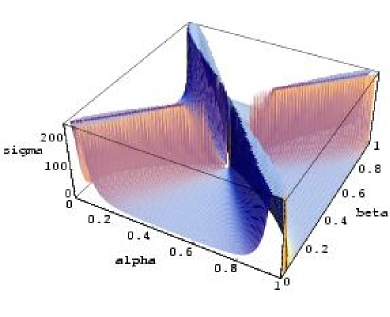
(a) $\alpha\in\left(0,1\right)$, $\beta\in\left(0,1\right)$

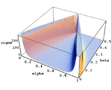
(b) $\alpha\in\left(0,1\right)$, $\beta\in\left(0,0.5\right)$

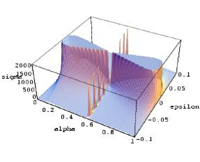
(c) $\alpha\in\left(0,1\right)$, $\beta=\alpha+\varepsilon$ with $\varepsilon\in\left(-0.1,0.1\right)$

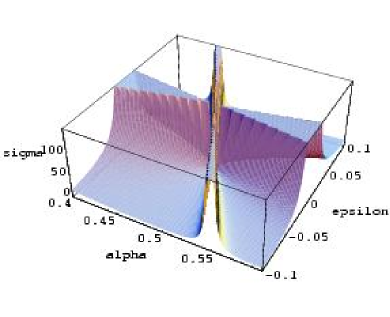
(d) $\alpha\in\left(0.4,0.6\right)$, $\beta=\alpha+\varepsilon$ with $\varepsilon\in\left(-0.1,0.1\right)$

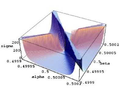
(e) $\alpha\in\left(0.4999,0.5001\right)$, $\beta\in\left(0.4999,0.5001\right)$

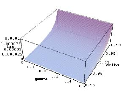
(f) $\gamma\in\left(0,0.5\right)$, $\delta\in\left(0.95,0.99\right)$

Figure 1: Kinematic plots of the $s$-wave cross-section $d\sigma/d\alpha$

The complete kinematic region is plotted in figure 1(a). Figure 1(b) shows a kinematic plot for $\alpha\in[0,1]$ and $\beta\in[0,1/2]$ (the units of $d\sigma/d\alpha$ are irrelevant for our kinematical discussion). One can easily see the symmetry $\alpha\leftrightarrow(1-\alpha)$. Further, the forward scattering poles $\alpha=\beta$ or $1-\alpha=\beta$ are clearly visible. Apart from these poles apparently no interesting structure is present at first glance. Numerical instability of the used Mathematica [21] routines leads to “holes” in that plot close to the forward scattering poles. Figure 1(c) zooms into that region with higher resolution. The interesting looking spoke-like structure corresponds again to forward scattering. However, figure 1(d) reveals the spokes as a numerical artifact (there should be a plateau instead). Plot 1(e) shows apparently self-similarity of the scattering amplitude: it looks identical to 1 (a), the plot showing the whole kinematic region, although the second one is zoomed in by a factor of 10000. This kind of self-similarity in the kinematic sector is a property of (6) which has not been discussed previously.

(a) $\alpha\in\left(0,0.9\right),\beta=\alpha+0.1$

(b) $\alpha\in\left(0.1,1\right),\beta=\alpha-0.1$

(c) $\alpha=0.5,\beta\in\left(0,1\right)$

(d) $\alpha\in\left(0,1\right),\beta=0.5$

(e) $\alpha=0.51,\beta\in\left(0,1\right)$

(f) $\alpha=0.5,\beta\in\left(0.49996,0.50004\right)$

Figure 2: Cuts through the kinematic plots

Before starting such a discussion we consider cuts through the kinematic plots, because they reveal a hidden substructure: figure 2(a) shows apart from the forward scattering pole two local maxima in the cross-section. The mirror counterpart is depicted in 2(b) – one sees clearly the symmetry between the graphs, a relic of the $\alpha\leftrightarrow(1-\alpha)$ symmetry. Since the center of the kinematic region ($\alpha\approx 0.5\approx\beta$) is not distinguishable very well in the previous plots some cuts through that region are helpful. The graphs 2(c) and 2(d) show, that the limiting value $\alpha=\beta=0.5$ seems to be finite. However, close to that value the forward scattering peaks still exist, as shown in 2(e). The final diagram 2(f) demonstrates the numerical instability close to the center. Of course, the spikes are artificial. Plugging the central values $\alpha=\beta=0.5$ into (6) yields a (pole-like) divergence which is not seen in 2(c) and 2(d), but this is due to the numerical instability shown in 2(f). So the forward scattering pole occurs also in the center of the kinematic region.

Surprisingly, the feature of self-similarity is absent in the cut graphs of figure 2. To resolve this puzzle it is helpful to reparameterize the scattering amplitude as a function of $\gamma=\alpha-1/2$ and $\delta=(\beta-1/2)/(\alpha-1/2)$ with the ranges $\gamma\in[-1/2,1/2]$ and $\delta\in[-\infty,\infty]$ (due to the symmetries in (6) it suffices to restrict oneself to the ranges $\gamma\in[0,1/2]$ and $\delta\in[0,\infty]$). Self-similarity of the cross-section (which now depends on $\gamma$ and $\delta$) would mean its independence of $\gamma$ (up to a scale factor). However, it is straightforward to check that (6) is not $\gamma$-independent. So why do we seem to observe self-similarity? The answer is contained in figure 1 (f) which plots the function $\tau(\gamma,\delta)$, defined by

$$\tau:=\frac{d\sigma}{d\alpha}(\gamma,\delta)/\frac{d\sigma}{d\alpha}(\gamma,\delta_{0}).$$ (7)

It is proportional to the cross-section (6) but rescaled such that at $\delta=\delta_{0}:=0.99$ (i.e. very close to the forward scattering peak) its value is fixed to 1 for all $\gamma$. Apparently, there is no $\gamma$ dependence visible in that plot, although a (hidden) substructure exists.

Analytically this can be seen most easily by expanding (6) close to $\delta=1$:

$$\frac{d\sigma}{d\alpha}=\frac{1}{\delta-1}A(\gamma)+B(\gamma)+{\cal O}(\delta-1),$$ (8)

with some simple but irrelevant functions $A(\gamma)$ and $B(\gamma)$. Plugging this result into (7) yields

$$\tau\approx\frac{(\delta_{0}-1)}{(\delta-1)}\left(1-(\delta_{0}-1)\frac{B}{A}\right)+(\delta_{0}-1)\frac{B}{A}+{\cal O}((\delta_{0}-1)^{2})\\ +{\cal O}((\delta-1)(\delta_{0}-1))+{\cal O}((\delta_{0}-1)^{3}/(\delta-1)).$$ (9)

For $\delta\approx\delta_{0}$ (this corresponds to the visually essential parts of the plots 1 (a) and (e)) the leading order (LO) is approximately 1 (and $\gamma$ independent) and the NLO vanishes. The self-similarity is broken only on the NNLO level in this kinematic region. Far away from the forward scattering peak the quantity $\tau$ is suppressed and deviations from self-similarity are present but not visible in the plots since they are scaled with $(\delta_{0}-1)$. Thus, we conclude that no (kinematic) self-similarity exists in our cross-section (6), but only a pseudo-self-similarity close to the forward scattering peaks.

As a final caveat we should emphasize that the full $4d$ theory – even in the special case of spherical symmetry – is more complex than the spherically reduced model we have treated. This is of particular importance at the quantum level [22, 23].

5 VBH geometry

Before we compare our VBH with Hawking’s VBH we would like to shed some light on the geometric role of its effective line element [9]:

$$(ds)^{2}=2drdu+\left(1-\frac{2m(r,u)}{r}-a(r,u)r\right)(du)^{2},$$ (10)

with $m(r,u):=\delta(u-u_{0})\theta(r_{0}-r)m_{0}(r_{0})$ and $a(r,u):=\delta(u-u_{0})\theta(r_{0}-r)a_{0}(r_{0})$. The $\theta$-function is responsible for a discontinuity: for $r\to\infty$ neither the Schwarzschild term proportional to $m$ nor the Rindler term proportional to $a$ is present. The $\delta$-function restricts the non-vacuum part to the outgoing null line depicted in figure 3 (the time reversed VBH is localized on an ingoing null line). The functions $m_{0}$ and $a_{0}$ are given by

$$m_{0}:=d_{1}r_{0}^{2}+d_{0}r_{0}^{3},\hskip 14.22636pta_{0}:=-2d_{1}+3d_{0}r_{0}.$$ (11)

It is amusing, that the “mass” $m_{0}$ does not only contain a “volume” term ($d_{0}r_{0}^{3}$) but also a “surface” term ($d_{1}r_{0}^{2}$).

Figure 3: CP diagram of the VBH

This line element was obtained in part by fixing the boundary values of the geometric quantities (thus our effective geometry is asymptotically flat per constructionem) and in part by reconstructing geometry out of the matter field (this was possible because we have treated the geometric part exactly; for details we refer to [9, 10]). The corresponding Carter-Penrose (CP) diagram is presented in figure 3.

It needs some explanations: first of all, the effective line element is non-local in the sense that it depends not only on one set of coordinates (e.g. ${u,r}$) but on two ($x=(u,r),y=(u_{0},r_{0})$). This non-locality was a consequence of integrating out geometry non-perturbatively [10]. For each selection of $y$ it is possible to draw an ordinary CP-diagram treating $u_{0},r_{0}$ as external parameters. The light-like “cut” in figure 3 corresponds to $u=u_{0}$ and the endpoint labeled by $y$ to the point $x=y$. The non-trivial part of our effective geometry is concentrated on the cut.

Of course, one should not look at the line elements in given coordinates, but at the scalar invariants of the Riemann tensor in order to obtain physical insight. For SRG it suffices to consider the Ricci-scalar, since there is only one independent physical quantity in the Riemann tensor. As inspection of the equations of motion for the spin connection immediately reveals (14), it has a distributional concentration at the endpoints of the cut and “propagates” along the light-like cut. This shows that the appearance of such a cut is not an artifact of the chosen coordinates, but has a physical counterpart in the curvature scalar (for details of that calculation we refer to appendix A):

$$R^{VBH}(u,r;u_{0},r_{0})=\delta(u-u_{0}){\Bigg{[}}-\delta^{\prime}(r-r_{0})\left(\frac{2m_{0}}{r}+a_{0}r\right)\\ -\delta(r-r_{0})\left(\frac{4m_{0}}{r^{2}}+6a_{0}\right)+\Theta(r_{0}-r)\frac{6a_{0}}{r}+2\frac{m_{0}}{r^{2}}\delta(r){\Bigg{]}}.$$ (12)

The last contribution corresponds to the Schwarzschild singularity and has been advocated in [24]. It is quite interesting to observe what happens when plugging (12) into the Einstein-Hilbert action ($\int_{0}^{\infty}dr\delta(r):=1$):

$$L^{VBH}_{EH}=\left.\int_{M_{4}}d^{4}x\sqrt{-g^{(4)}}R\right|_{VBH}=4\pi\int\limits_{-\infty}^{\infty}du\int\limits_{0}^{\infty}r^{2}drR^{VBH}(u,r;u_{0},r_{0})\\ =4\pi(2m_{0}+3a_{0}r_{0}^{2}-4m_{0}-6a_{0}r_{0}^{2}+3a_{0}r_{0}^{2}+2m_{0})=0.$$ (13)

It vanishes.

Apart from the cut, the spacetime coincides with (Minkowski) vacuum. It is fair to ask for precedents of such a geometry: on the one hand, our VBH seems similar to shock wave geometries (cf. e.g. [25]), but in our case the “shock” suddenly “evaporates” at $x=y$. In the matter sector, the VBH naturally shows resemblance to the quantum black hole obtained in the thin shell approach (cf. e.g. [26]) since in both cases the (spherically symmetric) shells are localized in space, but in our case the (off-shell) scalar field is additionally localized in time (cf. eq. (8) and (9) in [9]). On the other hand, – on a superficial level – our effective geometry could be interpreted as a soliton or an instanton solution since the non-vacuum part is “localized”, but as opposed to a soliton (localized on (a compact family of) time-like trajectories) or an instanton (localized in (Euclidean) space-time) we have a light-like localization, a “nulliton”, existing only for a finite affine parameter (which is roughly speaking the light-like “equivalent” of proper time) until it “evaporates” (thus, it is not stable as opposed to solitons). Moreover, our geometry is singular at $x=y$ and soliton solutions usually are required to be regular. The singularity appears to be an inevitable consequence of the light-like structure. So it seems this geometry is without precedent.

We do not want to suggest to take the effective geometry at face value – this would be like over-interpreting the role of virtual particles in a loop diagram. It is a nonlocal entity and we still have to “sum” (read: integrate) over all possible geometries of this type in order to obtain the nonlocal vertices and the scattering amplitude. But nonetheless, the simplicity of the effective geometry, the fact that one has to sum over all possible configurations and the vanishing of the Einstein-Hilbert action are nice qualitative features of this picture.

6 Comparison with Hawking’s VBH

We should clarify the difference between “our” VBH and “Hawking’s” VBH: while the latter is defined by its topological structure ($S^{2}\times S^{2}$) in Euclidean space [3] our definition relies on a discontinuity in a “phenomenological” quantity, the geometric part of the conserved quantity existing in all $2d$ dilaton theories [28, 29, 30]. In [31] its relation to ADM- and Bondi-mass as well as its equivalence with the so-called “mass-aspect function” is discussed. Since the latter has been used in numerical calculations as a signal for a black hole [32] we believe that the “BH” part in “VBH” is justified. As to “virtual” we would like to point out that asymptotically the geometry is equivalent to Minkowski spacetime. So a black hole does not exist in the initial or final states and appears only at an intermediate stage. This explains the notion “virtual”.

In this respect our VBH is quite similar to Hawking’s VBH. Also their corresponding topologies resemble each other: ours is $\Sigma\times S^{2}$, with $\Sigma$ being the (compact) light-like cut. Of course, there has to be a difference to the Euclidean $S^{2}\times S^{2}$ (where the notion of “light-like” does not exist, unless one complexifies) because after all our VBH inherits the Minkowski signature. Note that in both cases the first Betti number vanishes and the second is non-vanishing. This property was the main reason why Hawking considered $S^{2}\times S^{2}$ as an interesting building block of space-time foam [3].

Finally, let us address the issue of the two endpoints ($y$ and the intersection of the cut with the $r=0$ line) of the cut, which are obviously absent in the Euclidean version: we have already emphasized that our calculations have been performed in a specific gauge. In other words, a peculiar slicing has been introduced. If one would slice an $S^{2}$ one would also obtain two “endpoints” corresponding to the intersection points of the two tangential hyper-planes in the family of parallel hyper-planes slicing the 2-sphere. This shows that the two notions of VBH are not completely different after all.

7 Outlook

We have shown that virtual black holes (VBHs) provide non-trivial phenomenology already in the simple case of the spherically reduced Einstein-massless-Klein-Gordon model. They enter the $S$-matrix, an idea put forward some time ago in [11]. Of course, $4d$ gravity – even in the spherically symmetric case – is more complex and classical equivalence to a $2d$ theory by no means implies quantum equivalence since, roughly speaking, renormalization and dimensional reduction need not commute (“dimensional reduction anomaly” [22, 23]). But since our results were obtained for the low energy limit any UV cut-off dependency should be irrelevant for us. So it is likely that similar features as discussed in the present and previous work [9] (forward scattering, decay of $s$-waves) will occur in the full $4d$ theory close to spherical symmetry.

We extended the discussion of [9, 10] and found $CPT$ invariance of the cross-section (6). Moreover, we found pseudo-self-similar behavior and non-trivial substructure (which breaks that self-similarity) in its kinematic sector. Together with the monomial energy scaling behavior this might lead towards an easier derivation of the simple result (4), if one could prove these properties from first principles.

We studied the VBH geometry (10) in some detail (including the presentation of a Carter-Penrose diagram despite its non-local nature) and found distributional contributions to the ensuing Ricci-scalar (12). The corresponding Einstein-Hilbert action (13) was found to be vanishing.

Finally, we compared our notion of VBHs with Hawking’s Euclidean bubble definition [3]. We found parallels in the topological structure. Still, the two notions are quite different, since our results cannot be continued straightforwardly to Euclidean space (there are no Minkowskian instantons).

Within our perturbation theory there are two logical next steps: one could consider additional external scalar fields at tree level or start with one-loop calculations. The first route would be straightforward, but since already the 4-point vertex at tree level involved quite lengthy transformations and little new is to be expected from such a calculation this would probably be a misdirection of resources. Moreover, the contribution to the amplitude will be suppressed by additional powers of the total energy. The only relevant issue could be a sizable contribution in a region where our 4-point cross-section was almost vanishing. The loop calculation, however, seems more interesting, at least as far as the physical content is concerned: we would gain further insight into the information paradox in a region, which is usually not easily accessible to standard black hole physics: microscopic black holes (with total mass much smaller than Planck mass). Preliminary results look promising [33].

It would also be of interest to consider fermions. We expect qualitative changes due to the following observations: on the one hand, the constraint algebra will be quite different – we already have witnessed the tremendous change between minimal and nonminimal coupling. On the other hand, our amplitude (4) contains in the language of elementary particle physics the sum over all channels ($s$, $t$, and $u$). However, with a conserved charge (like fermion number) typically a sum over only two channels occurs (cf. e.g. [34]). Moreover, the dimensional reduction procedure is more involved for this case since one has to consider the spin structure. Roughly speaking, fermions “feel” the underlying geometry much more than scalar particles. In particular, terms coupled to the auxiliary fields $X^{\pm}$ and a dilaton dependent “mass” term will appear in the matter Lagrangian [35]. So new results are to be expected from $s$-wave fermion scattering.

A final ceterum censeo: as long as a comprehensive quantum theory of gravity does not exist, $2d$ dilaton gravity will remain an active field trying to solve the conceptual issues of quantum gravity in a technically more manageable framework.

Note added in proof: According to an erratum to [9] (which is in the process of publication) the line element (10) should read $(ds)^{2}=2drdu+(1-2m(r,u)/r-a(r,u)r-d(r,u))(du)^{2}$ with $d(r,u):=\delta(u-u_{0})\theta(r_{0}-r)d_{0}(r_{0})$. This leads to additional contributions to the Ricci scalar (12) which can be calculated with the methods described in appendix A. The result is $R_{\rm new}=R_{\rm old}+\delta(u-u_{0})\left[-\delta^{\prime}(r-r_{0})d_{0}-\delta(r-r_{0})4d_{0}/r+\theta(r_{0}-r)2d_{0}/r^{2}\right]$. However, these new terms do not change any of the conclusions of the present work (in particular, the action (13) still vanishes).

Appendix A - curvature of VBH geometry

For a primitive discussion of the Ricci-scalar we need only the equation of motion following from (2) when varying the dilaton field $X$:

$$d\wedge\omega-e^{-}\wedge e^{+}\left(V^{\prime}(X)+X^{+}X^{-}U^{\prime}(X)\right)+\frac{\delta{\cal{L}}^{(m)}}{\delta X}=0,$$ (14)

The first observation is that the last term $\delta{\cal L}^{(m)}/\delta X$ contains $\delta$-like contributions. This follows from equations (8) and (9) of [9], which localize the trace of the $4d$ energy-momentum tensor (which is proportional to the term $\delta{\cal L}^{(m)}/\delta X$). The second observation concerns the relation between the Ricci-scalar and the first term, $d\wedge\omega$: they are (apart from numerical pre-factors) Hodge dual to each other. This implies that the Ricci-scalar has a $\delta$-like contribution at the point denoted by $y$ in figure 3. The second term has a discontinuity at the same point, inherited from the discontinuity in the metric. The curvature vanishes trivially beside the cut and it is non-vanishing on the cut. That is why we said the curvature singularity at $y$ “propagates” along the light-like cut to the origin. Alas, there is a “subtlety” involved in this discussion: one term contains the product of two $\delta$-functions at the same point, i.e. it is not a well-defined distribution.

Therefore, we will discuss the curvature forgetting about the first order formalism and start directly with the line element (10) supplemented by the angular part $-r^{2}d^{2}\Omega$. In complete analogy to [24] we use the Kerr-Schild decomposition $g_{ab}=\eta_{ab}-fk_{a}k_{b}$ (note the relative sign due to differing signature conventions between this work and [24]) with the profile function $f$, a null vector field $k_{a}$ and a flat background metric $\eta_{ab}$. This representation is tailor-made for distributional contributions in $f$, since the Ricci scalar ($k^{a}=\eta^{ab}k_{b}=g^{ab}k_{b}$)

$$R=\partial_{a}\partial_{b}\left(fk^{a}k^{b}\right)$$ (15)

contains the profile function linearly and hence problems with “squared $\delta$-functions” will not arise. Using again outgoing Sachs-Bondi coordinates $(ds)^{2}=2drdu+(du)^{2}-f(du)^{2}$ the profile function reads

$$f=\left(\frac{2m_{0}}{r}+a_{0}r\right)\delta(u-u_{0})\Theta(r_{0}-r),$$ (16)

and as additional simplifications we have $(k\cdot\partial)=\partial_{r}$ and $(\partial\cdot k)=2/r$. Thus, we obtain

$$\left.R\right|_{r>0}=\partial_{r}\partial_{r}f+\frac{4}{r}\partial_{r}f+\frac{2}{r^{2}}f=\delta(u-u_{0}){\Bigg{[}}-\delta^{\prime}(r-r_{0})\left(\frac{2m_{0}}{r}+a_{0}r\right)\\ -\delta(r-r_{0})\left(\frac{4m_{0}}{r^{2}}+6a_{0}\right)+\Theta(r_{0}-r)\frac{6a_{0}}{r}{\Bigg{]}}.$$ (17)

According to [24] we will obtain in addition a $\delta$-like contribution at the origin (the Schwarzschild singularity) of the form $\left.R\right|_{SS}=\delta(u-u_{0})\delta(r)2m_{0}/r^{2}$ with $\int_{0}^{\infty}dr\delta(r):=1$. Thus, the curvature scalar is really concentrated on the light-like cut depicted in figure 3 with distributional contributions on its endpoints and it vanishes for $r>r_{0}$. Note that the only nonvanishing contribution along the cut is due to the Rindler term (this follows simply from $\left.R\right|_{r>0}=0$ for Schwarzschild geometry).

References

- [1] J.A. Wheeler. Geometrodynamics and the issue of the final state. In C. DeWitt and B.S. DeWitt, editors, Relativity, Groups and Topology, page 316. Gordon and Breach, New York, 1964.
- [2] Carlo Rovelli. Loop quantum gravity. Living Rev. Rel., 1:1, 1998.
- [3] S. W. Hawking. Virtual black holes. Phys. Rev., D53:3099–3107, 1996.
- [4] S. W. Hawking and Simon F. Ross. Loss of quantum coherence through scattering off virtual black holes. Phys. Rev., D56:6403–6415, 1997.
- [5] John R. Ellis, J. S. Hagelin, D. V. Nanopoulos, and M. Srednicki. Search for violations of quantum mechanics. Nucl. Phys., B241:381, 1984.
- [6] F. Benatti and R. Floreanini. Massless neutrino oscillations. Phys. Rev., D64:085015, 2001.
- [7] Patrick Huet and Michael E. Peskin. Violation of CPT and quantum mechanics in the K0 - anti-K0 system. Nucl. Phys., B434:3–38, 1995.
- [8] F. Benatti and R. Floreanini. Non-standard neutral kaons dynamics from infinite statistics. Annals Phys., 273:58–71, 1999.
- [9] P. Fischer, D. Grumiller, W. Kummer, and D. V. Vassilevich. S-matrix for s-wave gravitational scattering. Phys. Lett., B521:357–363, 2001.
- [10] Daniel Grumiller. Quantum dilaton gravity in two dimensions with matter. PhD thesis, Technische Universität Wien, 2001. preprint gr-qc/0105078.
- [11] G. ’t Hooft. The scattering matrix approach for the quantum black hole: An overview. Int. J. Mod. Phys., A11:4623–4688, 1996.
- [12] D. Grumiller, W. Kummer, and D. V. Vassilevich. The virtual black hole in 2d quantum gravity. Nucl. Phys., B580:438–456, 2000.
- [13] D. Grumiller. The virtual black hole in 2d quantum gravity and its relevance for the S-matrix. 2001. Talk given at the Fifth Workshop on Quantum Field Theory under the Influence of External Conditions, to appear in Int.J.Mod.Phys.A, preprint hep-th/0111138.
- [14] Peter Schaller and Thomas Strobl. Poisson structure induced (topological) field theories. Mod. Phys. Lett., A9:3129–3136, 1994.
- [15] Thomas Strobl. Gravity in two spacetime dimensions. 1999. Habilitation thesis, preprint hep-th/0011240.
- [16] Thomas Klösch and Thomas Strobl. Classical and quantum gravity in (1+1)-dimensions. Part 1: A unifying approach. Class. Quant. Grav., 13:965–984, 1996.
- [17] W. Kummer, H. Liebl, and D. V. Vassilevich. Exact path integral quantization of generic 2-d dilaton gravity. Nucl. Phys., B493:491–502, 1997.
- [18] W. Kummer, H. Liebl, and D. V. Vassilevich. Integrating geometry in general 2d dilaton gravity with matter. Nucl. Phys., B544:403–431, 1999.
- [19] Peter Fischer. Vertices in spherically reduced quantum gravity. Master’s thesis, Vienna University of Technology, 2001.
- [20] R. F. Streater and A. S. Wightman. PCT, spin and statistics, and all that. Redwood City, USA: Addison-Wesley (Advanced book classics), 1989.
- [21] S. Wolfram. The Mathematica book. Wolfram Media, Illinois and Cambridge University Press, Cambridge, 4 edition, 1999.
- [22] V. Frolov, P. Sutton, and A. Zelnikov. The dimensional-reduction anomaly. Phys. Rev., D61:024021, 2000.
- [23] P. Sutton. The dimensional-reduction anomaly in spherically symmetric spacetimes. Phys. Rev., D62:044033, 2000.
- [24] Herbert Balasin and Herbert Nachbagauer. Distributional energy momentum tensor of the Kerr-Newman space-time family. Class. Quant. Grav., 11:1453–1462, 1994.
- [25] P. C. Aichelburg and R. U. Sexl. On the gravitational field of a massless particle. Gen. Rel. Grav., 2:303–312, 1971.
- [26] V. A. Berezin, A. M. Boyarsky, and A. Yu. Neronov. Quantum geometrodynamics for black holes and wormholes. Phys. Rev., D57:1118–1128, 1998.
- [27] J. Polchinski. String theory volume I. Cambridge, UK: Univ. Pr. (1998).
- [28] Wolfgang Kummer and Dominik J. Schwarz. Renormalization of R**2 gravity with dynamical torsion in d = 2. Nucl. Phys., B382:171–186, 1992.
- [29] Harald Grosse, Wolfgang Kummer, Peter Presnajder, and Dominik J. Schwarz. Novel symmetry of noneinsteinian gravity in two- dimensions. J. Math. Phys., 33:3892–3900, 1992.
- [30] W. Kummer and P. Widerin. Noneinsteinian gravity in d=2: Symmetry and current algebra. Mod. Phys. Lett., A9:1407–1414, 1994.
- [31] D. Grumiller and W. Kummer. Absolute conservation law for black holes. Phys. Rev., D61:064006, 2000.
- [32] Matthew W. Choptuik. Universality and scaling in gravitational collapse of a massless scalar field. Phys. Rev. Lett., 70:9–12, 1993.
- [33] D. Grumiller, W. Kummer, and D. Vassilevich. in preparation.
- [34] M. E. Peskin and D. V. Schroeder. An Introduction to Quantum Field Theory. Addison-Wesley Publishing Company, 1995.
- [35] D. Hofmann. personal communication.