Lighthouses of Gravitational Wave Astronomy

Abstract

Gravitational wave detectors capable of making astronomical observations could begin to operate within the next year, and over the next 10 years they will extend their reach out to cosmological distances, culminating in the space mission LISA. A prime target of these observatories will be binary systems, especially those whose orbits shrink measurably during an observation period. These systems are standard candles, and they offer independent ways of measuring cosmological parameters. LISA in particular could identify the epoch at which star formation began and, working with telescopes making electromagnetic observations, measure the Hubble flow at redshifts out to 4 or more with unprecedented accuracy.

1 Introduction

Gravitational wave interferometers now under construction at several locations around the world will soon begin making observations. Although their initial sensitivities will be marginal, a planned program of upgrades and technology development will make them powerful instruments of cosmology over the next decade. In 2011 the launch of the joint ESA-NASA gravitational wave observatory LISA will extend the reach of this form of astronomy to the entire observable universe.

Astronomy has consistently proved itself to be full of surprises for observations in new wavebands, and this may well also be true for gravitational wave astronomy. Therefore it is a little dangerous to try to predic what these new detectors will observe, but it is useful to look ahead at this point. In particular it is not too early to consider and even to begin to plan the ways in which gravitational wave detectors and other astronomical telescopes could work together.

For cosmology, one of the most interesting features of gravitational wave observations is that certain systems are standard candles: their distance can be inferred from their gravitational waveforms. These systems are chirping binaries, that is binary systems whose orbits shrink during the observations time because of the energy they lose to gravitational waves. The change of the orbit raises the frequency of the gravitational wave, producing a “chirp” waveform.

In this review I will point out a number of ways in which gravitational wave observations of these chirping waveforms, usually coupled with coordinated observations in electromagnetic wavebands, can be used to provide cosmological information. For example, chirps from neutron-star binaries in the last few minutes before coalescence should be observed frequently by advanced ground-based detectors. These detectors can give astronomers advance notice of and rough positions for such inspiral events, and optical identifications of any afterglows produced by the mergers of the neutron stars will sharpen the distance estimate made by the detectors. Redshifts to the afterglows can be used with these distance estimates to provide independent measurements of the Hubble constant to accuracies of a few percent, and of the acceleration of the universe out to redshifts of order 0.2. Chirps from mergers of stellar-mass black holes could, even in the absence of electromagnetic counterparts, provide estimates of the cosmological acceleration out to redshifts of order 1.

Chirps from very massive ($1000\,M_{\odot}$) black hole binaries that might have formed in the first epoch of star formation, observed by LISA, could be used to determine when star formation began. Chirps from the coalescences of massive black holes in galactic centres, again observed by LISA, could measure the cosmological deceleration out to redshifts of 4 or more, provided that electromagnetic observations can pin down the cluster of galaxies in which a coalescence occurred. This will be a real challenge to astronomy but it could have an immense payoff.

Before discussing these possibilities, I begin this article with two background sections. The first reviews gravitational wave astronomy, particularly emphasising the ways in which gravitational wave observations differ in concept and information content from electromagnetic observations, and outlining the development of detectors and the timetable on which sensitivity improvements can be expected. The second iss an introduction to chirp waveforms and the kind of information they carry. These two sections prepare for the subsequent discussions of how cosmological information can be extracted from gravitational wave observations.

2 Gravitational wave observing

The principles of interferometric detectors and their current development are reviewed in a number of places in the literature [1, 2]. In particular, [2] contains references to the recent literature. Several accessible textbooks [3, 4] review the principles of gravitational radiation, and two recent encyclopedia articles also address these issues [5, 6]. What follows here is a brief introduction to these subjects.

2.1 Action of waves on a detector

Figure 1 shows how gravitational waves act on a ring of free particles. The action is by tidal forces carried by the waves, which distort the ring in directions transverse to the direction of propagation of the wave. Because of the equivalence principle, the overall acceleration of the ring produces no local effects; the only measurable effects are in the relative distortions. Therefore the linear displacements of these distortions are proportional to the size of the ring: the larger the ring, the larger the displacement.

The figure can be viewed as an elementary detector. By sensing the relative displacements of particles on the ring, one can measure the wave. This is exactly how interferometric detectors work. They use laser interferometry to measure changes in the relative distances between the central particle of a ring and two particles in orthogonal directions along the circumference of the ring. The particles are mirrors in the interferometer that are free to move along the direction of the displacement.

Older, solid-mass detectors, called bar detectors, use the stretching along one diameter of the ring. The restoring forces of the solid material means that the response to the wave is more complicated than in an interferometer, but the principle is the same.

All proposed gravitational wave detectors are linearly polarized. To measure the polarization of a wave requires either that several detectors make measurements or that the wave lasts long enough so that the motion of a detector carried by the Earth or in a space orbit changes the projected polarization of the detector, allowing it to measure two independent polarizations.

The waveforms in Fig. 1 have a simple relationship to the mass motions in the source of the gravitational wave [7]. They mimic any oscillating motions in the source, as projected on the plane of the sky as seen by the ring. If the motions are all along one line, then the polarization ellipse will have its alternating major/minor axes along that line. If the motions are circular, then the wave will have circular polarization, which is a linear combination of the two polarizations with a phase shift of 90 degrees. Thus, measuring the polarization of a gravitational wave allows one to make direct inferences about the source, such as measuring the angle of inclination of the orbital plane of a binary system.

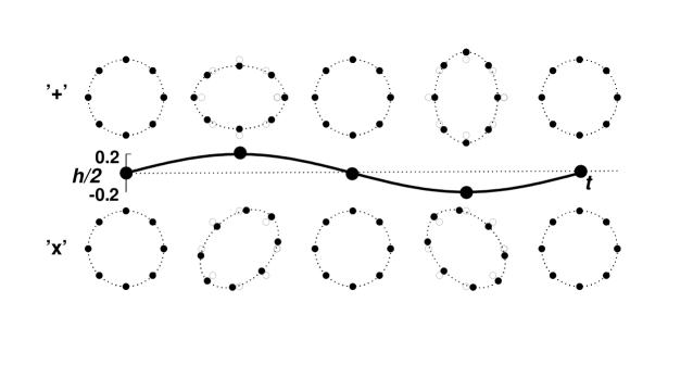
Figure 1: Two independent polarisations of a plane gravitational wave are illustrated by their actions on a ring of free particles in empty space. The waves act transversely, so in this figure the waves approach perpendicular to the paper. The waves distort the ring into ellipses with alternating major and minor axes. The two polarizations are orthogonal because the ellipses are rotated by $45^{\circ}$ with respect to one another. The action of any plane wave is a superposition of these two polarizations. The waves act through tidal forces, so the stretching is proportional to the size of the ring: a given gravitational wave will produce twice the relative displacement in a ring twice the size. The waveform in the centre shows the size of the strain illustrated here, which is defined as half of the amplitude $h$ of the wave. (This is much larger than we expect, of course.) The distortions produced by a given wave mimic the motions in the source of the wave as projected onto the plane of the sky as seen from the ring of particles. For example, if the source contains stars moving back and forth along the $x$-axis, then the wave will produce a similar motion in the ring (top line).

2.2 Planned ground-based detectors

I will focus here on the planned interferometers, which have the biggest potential for astronomical and particularly for cosmological observing. There are four instruments now being built [2] that should reach the target sensitivity of first-generation detectors: to measure $h\sim 10^{-21}$. This is a threshold that has been the goal of detector development for decades: it is the largest amplitude that could reasonably be expected from sources that might be observable in one year. Observing at this level gives no guarantees of detections: Nature has to cooperate by providing strong sources. These first-generation detectors are the first step along a planned sequence of sensitivity improvements that will produced essentially guaranteed detections by the end of this decade.

Interferometers use light to compare the lengths of the two arms. The fundamental limit on sensitivity is the amount of light, since quantum uncertainties in the arrival times of photons produce a stochastic noise called shot noise, which is less important when there are more photons. However, the main technical challenge to these detectors is to eliminate low-frequency noise from external vibrations and from internal thermal vibrations of the components [2]. These noise sources will set a lower-frequency limit of about 40 Hz on LIGO and GEO. The VIRGO detector is investing more effort in controlling vibration noise, and will have some sensitivity even at 20 Hz. All detectors go up to a few kHz before shot noise limits their sensitivity.

The largest and most ambitious project is LIGO, an American project building two 4-km detectors, one at Hanford (WA) and the other at Livingston (LA). The Hanford detector also contains a 2-km instrument for local coincidence and anti-coincidence observing. LIGO is now successfully doing interferometry, and is improving its sensitivity and reliability. LIGO may begin taking data at its planned sensitivity within the next year.

The next-largest instrument under construction is VIRGO, near Pisa. It is a cooperation between France and Italy. The timescale for operation of this 3-km instrument is about a year behind LIGO.

In Germany the GEO project is building a smaller detector, GEO600, with 600-m arms, that will nevertheless have a similar sensitivity to the LIGO instruments, and which is on the same timescale as LIGO. It achieves this sensitivity by using more advanced optical and mechanical technology. This technology will be transferred to LIGO and VIRGO when they are ready for upgrades to higher sensitivity.

GEO600 and LIGO are planning a joint test data run in December 2001, and the two projects have in fact signed a strong data-sharing and data-analysis MOU, providing for joint publication of all results. Other projects have been invited to join in this agreement.

The second-generation instruments will be upgrades of LIGO and VIRGO, which could be in place by 2007, plus a proposal in Japan that is not yet funded. These will improve the first-generation sensitivity by a factor of 10 in amplitude, and they will push the observing frequency limit down to perhaps 10 Hz. Scientists are beginning to design radical new technology for the third generation, envisioning yet a further step by a factor of 10, and a further broadening of the observing frequency window. It is possible that VIRGO and GEO will cooperate on a joint proposal for a new third-generation detector in Europe.

2.3 LISA, the first space-based detector

Ground-based detectors will never have sufficient sensitivity to do useful work below about 1 Hz, because gravity noise generated by moving masses on the Earth will be larger in amplitude than expected gravitational waves. Since gravity cannot be screened, the only solution is to put the detector into space. This is the justification for LISA, which is planned for launch in 2011. Unlike the ground-based detectors, LISA will observe many of its sources with extremely high signal-to-noise ratio. LISA is likely to be the first of a sequence of space-based detectors over the next few decades. LISA could have a mission lifetime of up to 10 years. The state of development was reviewed recently in the proceedings of the Third International LISA Symposium [8].

LISA began in 1993, when an American group led by P Bender of JILA, which had been studying space-based detectors for some time, encouraged a group of Europeans, largely in the GEO and VIRGO projects, to propose a detector for the ESA M3 mission opportunity. The mission was not selected because it was too expensive for this medium-mission limit, but the scientific potential was regarded so highly that the group was encouraged to propose for the Horizon 2000+ Cornerstone selection in 1995. The present design, based on a triangular three-armed interferometer, with a detailed plan for the optics and sensing needed, matured for that proposal.

LISA was indeed selected as a Cornerstone, but still the costs were troubling. A redesign by the European LISA team, cooperating with JPL and Bender’s group at JILA, produced the current baseline design using three spacecraft, and seemed to be affordable. The project meanwhile gained considerable interest among astronomers, who were coming to the conclusion that the giant black holes that LISA could observe were ubiquitous in the centres of galaxies. This led to efforts to bring NASA into the project to share costs.

Earlier this year (2001), ESA and NASA exchanged letters of agreement to share the project equally, and ESA invited NASA to contribute to a technology demonstration mission called SMART 2, due for launch in 2006. The technology of LISA is a fascinating subject in itself, which there is no room for here. The two agencies have formed a joint LISA International Science Team (LIST), that will organise the community. It has two chairs, T Prince (Caltech and JPL) and K Danzmann (of the new branch of the Albert Einstein Institute in Hannover). Theorists and astronomers who want to contribute to the science required before LISA’s launch are welcomed to join in the projects being encouraged by the LIST’s Sources and Sensitivities Working Group, jointly chaired by S Phinney (Caltech) and the present author.

As mentioned above, LISA is a three-armed detector. The roughly equilateral triangle maintains its shape as the three spacecraft follow their independent orbits around the Sun. The triangle lies in a plane tilted $60^{\circ}$ to the ecliptic, and is situated about $20^{\circ}$ behind the Earth in its orbit. The arm-length of 5 million kilometres permits good sensitivity below 0.1 Hz. The lower limit on LISA’s frequency window is about 0.1 mHz, where perturbations due to fluctuations in the solar radiation pressure dominate. Figure 2 shows the way the location and orientation of LISA change during a year.

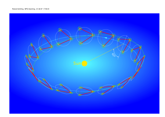
Figure 2: LISA’s configuration remains roughly equilateral and turns about an axis perpendicular to the triangle’s plane, while the triangle remains in a plane tilted $60^{\circ}$ to the ecliptic as the spacecraft orbit the Sun in one year.

2.4 Principles of observation with gravitational waves

Gravitational wave observing is rather different from observing in the electromagnetic spectrum. This is partly because detectors cannot be pointed: they are simple quadrupoles with broad response patterns on the sky. And it is partly because detectors register the waves coherently, following the oscillations of phase. By contrast, most electromagnetic detection is bolometric, registering the energy and not the phase. Even radio interferometry, which uses phase at an early stage, eventually rectifies the signal and records the energy in the fringes. Detectable electromagnetic waves simply oscillate too fast to be recorded, and their phase in any case does not necessarily contain important information.

The gravitational wave phase oscillated at kHz frequencies or lower, and directly reflects the mass motions in the source. Almost all the useful information in a signal is in the phase $\phi(t)$. This has several implications that are not immediately obvious to astronomers used to electromagnetic observing.

First, spectroscopy and polarimetry are automatic. The detectors are linearly polarised, and spectroscopy is nothing more than taking the Fourier transform of the detected signal.

Second, detecting a gravitational wave usually means being able to measure several parameters, such as the masses of the systems, that are encoded in the phase and frequency information. Moreover, as explained earlier, the polarisation information can be used to infer source orientations.

Third, observing by multiple detectors brings great benefits, particularly in angular resolution, as well as in confidence when signals are weak. The angular resolution improvements are analogous to what happens in radio interferometry. Even single detectors can achieve this if they observe a continuous source long enough to take advantage of the changing detector position; in this case such a detector effectively does aperture synthesis by itself.

Fourth, data analysis on computers plays a crucial role in detection. The optimum detection strategy in gravitational wave observing is to employ matched filtering [9]. This means comparing the observed phase $\phi_{\text{true}}(t)$ with the expected phase of a template signal $\phi_{\text{template}}(t)$. If the two match well enough, which usually means that $|\phi_{\text{true}}(t)-\phi_{\text{true}}(t)|<1\,\text{radian}$ over the signal duration, then one is close to optimal. Since the templates depend on parameters, which describe physical properties like sky location, source masses, orbit spindown, and other effects, a search for signals typically involves many repeated comparisons with slightly different templates. Then the availability of computer power (or the lack of it) can limit the sensitivity of an observation. This sometimes happens for other kinds of observing, for example the search for binary radio pulsars, where the parameter space that must be searched for signals is non-trivial in size.

Fifth, gravitational wave astronomers always speak about detecting amplitudes, not energy. This means their signal-to-noise ratios are the square-roots of energy or flux-based signal-to-noise measures. So if a gravitational wave observation with LISA can reach a signal-to-noise ratio of $10^{4}$, then this should be compared with an optical observation with a ratio of $10^{8}$: one photon of background for each $10^{8}$ photons from the source! This is suggestive of how much detailed information is potentially extractable from LISA observations.

There are many analogies between long-duration gravitational wave observations and radio observations of pulsars, in that radio observations are coherent as regards the pulse period itself. This is similar to the gravitational wave period of waves from the same pulsar, so many issues are the same. For example, gravitational wave positions will be at the same accuracy level as radio positions, around the arcsecond mark.

2.5 Angular positions

Once a source of gravitational waves has been detected, the most important information that the observation can produce is, of course, the location of the source on the sky. The accuracy of angular positions will be the crucial step in identifying sources and opening them for study by electromagnetic observation.

Since, as we remarked above, the pointing accuracy of an individual detector is poor over a short observation time, the position of the source must use more information than the instantaneous response of a single detector. The accuracy of locating a short burst comes entirely from the simultaneous observation of the event by several detectors. The accuracy of a long-duration observation is achieved, as mentioned above, by aperture synthesis.

A short burst may be defined as one in which the acceleration of the detector during the observation does not produce an overall phase-shift of the wave-form by more than one radian. The overall motion of the detector produces a constant (and usually unobservable) Doppler effect, but the acceleration of the detector distorts the waveform, and this can tell us where the wave came from. If the detector acceleration is $\vec{a}$ and the wave-vector of the radiation from the source is $\vec{k}$, then during an observation lasting a time $T$, short enough to regard the acceleration as constant, the phase-shift induced by the acceleration is

$$\Delta\phi_{\text{accel}}=\frac{1}{2}(\vec{a}\cdot\vec{k})T^{2}.$$

The condition that this should be less than 1 amounts, for a typical value of the gravitational wave frequency $f_{\text{gw}}$ and for the acceleration produced by the rotation of the Earth, this sets a limit on the time of observation of

$$T_{\text{burst}}<56\left(\frac{f_{\text{gw}}}{1\,\text{kHz}}\right)^{-1/2}\,\text{min}.$$ (1)

For such bursts, the position must be triangulated by using the arrival times of the waves at several detectors. This uses the detectors as an interferometer array, and the pointing accuracy is the diffraction limit, roughly the wavelength of the waves divided by the detector spacing. Within this, a source with strong signal-to-noise ratio can be located more accurately. If SNR is the amplitude signal-to-noise ratio for a particular observation, then for detectors with a baseline between Europe and the USA, say $10^{4}$ km, the accuracy is [10]

$$\Delta\theta_{\text{burst}}\sim\frac{2^{\circ}}{\text{SNR}}\left(\frac{f_{\text{gw}}}{1\,\text{kHz}}\right)^{-1}.$$ (2)

A confidence limit for detection will be something like $\text{SNR}>5$, so that any detected source might be triangulated to better than half a degree. A strong source with $\text{SNR}=20$ could be located to within 5 to 10 arcminutes.

These are overly optimistic numbers, however, because there is covariance with other observational errors. If there is an error in determining the polarisation, then this could masquerade as a delay or advance in the signal by up to half a cycle. What is more, the diffraction limit applies only if there are enough detectors to determine the polarisation. With three detectors there are two possible solutions to the location on the sky. The ambiguity is resolved only with four or more detectors. Moreover, if the detectors are unusually well aligned, then they do not determine polarisation as well. Unfortunately this is the case: the LIGO detectors, in the interests of ensuring that they should see nearly identical responses, are very well aligned, so they do not contribute much to a position determination. The result is that real position determinations for bursts might be five to ten times worse than the numbers quoted above.

This situation could be significantly improved if a detector is built in Japan, with its long baseline to the others. Such a detector would improve both the detection rate and the position determinations by a factor between two and four.

A long-duration source permits a single detector to determine the position by using the phase-modulation and time-dependent polarisation projection to measure both the polarisation and position jointly. The best case is when the source lasts for a year, so that the detector synthesises a telescope with an aperture of 2 AU. The diffraction-limited position accuracy improves on the above to

$$\Delta\theta_{\text{continuous}}\sim\frac{0.5\,\text{arcsec}}{\text{SNR}}\left(\frac{f_{\text{gw}}}{1\,\text{kHz}}\right)^{-1}.$$ (3)

Again, this is a little optimistic because polarisation errors can add up to a cycle to the waveform. But the pointing accuracy for ground-based detectors observing pulsars, for example, is very good. However, LISA will observe in the mHz region, which degrades its position accuracy. This is compensated somewhat by the large SNR, so that the result is a resolution accuracy between 10 arcminutes and 10 degrees, depending on how strong the source is. We will come back to the importance of these errors in the next section.

2.6 Amplitude estimates

The use of chirping binaries as standard candles depends on being able to measure the amplitude of their radiation accurately. In principle, this is just what the SNR measures, so the amplitude error would be of order $1/\text{SNR}$. But there is a strong covariance with the position error, since the antenna pattern of the detectors is broad. Roughly speaking, a position error of $\Delta\theta$ measured in radians produces a relative change in the sensitivity of the detector with respect to the source by a comparable amount. This will result in a wrong determination of the amplitude. So a good rule of thumb for amplitude errors is:

$$\Delta h=\max(1/\text{SNR},\Delta\theta).$$ (4)

If the only observations of the event are from gravitational wave detectors, then $\Delta\theta$ must be inferred from the equations above. But if the event can be identified by electromagnetic observations, then the position accuracy can be much improved, and with it the amplitude accuracy. This is particularly the case for LISA, where the SNR could be as high as $10^{4}$, but the intrinsic position accuracy could be as bad as 0.2 radians [11]. The astronomical return from LISA observations can be greatly improved by coordinated electromagnetic observations.

3 Chirping Binaries

3.1 Distance determination: the standard candle

When LISA or a network of ground-based detectors observes a binary system, then they can determine the angular position, amplitude, and angle of inclination of the binary orbit, as described above. For simplicity let us now assume that the orbit is circular, although what we describe can be extended to elliptical orbits.

There is a remarkable coincidence in the radiation from binary systems, in that both the amplitude $h$ of the radiation and the rate of change of the frequency of the radiation $df_{\text{gw}}/dt$ depend on the masses of the two stars only through exactly the same combination, which is called the chirp mass M of the system. If the two stars have masses $m_{1}$ and $m_{2}$, with associated reduced mass $\mu$ and total mass $M_{T}$, then the chirp mass is defined by

$${\mathcal{M}}:=\mu^{3/5}M_{T}^{2/5}=(m_{1}m_{2})^{3/5}(m_{1}+m_{2})^{-1/5}.$$ (5)

This was first pointed out by the present author [12], who suggested how this could be used to measure the luminosity distance $d_{L}$ to any binary system that chirped, that is whose $df_{\text{gw}}/dt$ could be measured.

One way to see how this can be done is to consider the formula for the SNR of an observation using a filter that has been perfectly matched to the incoming signal, in polarisation and chirp mass. We consider only the radiation from the orbit, not from the later coalescence event. This underestimates the SNR, but it has the advantage that the orbit is fully understood and its SNR can be characterised, while the radiation to be expected from coalescence is not yet known. Then the SNR can be written in the following way for a burst chirp  [13], that is a chirp that lasts less than the time given in (1):

$$\text{SNR}=8\Theta\frac{r_{0}}{d_{L}}\left(\frac{{\mathcal{M}}}{1.2M_{\odot}}\right)^{5/6}\zeta(f_{\text{max}}).$$ (6)

The following terms enter this equation:

• $\Theta$ is a factor that depends on the projection of the polarisation of the wave on the antenna pattern, so it is a function of the orientation of the binary relative to the detector. This is measurable from the polarization and direction information.

• $r_{0}$ is the range of the detector for this kind of observation, that is a distance that depends on the sensitivity of the detector. It is a function only of the detector.

• $d_{L}$ is the luminosity distance to the source, and is what we want to determine from the observation.

• ${\mathcal{M}}$ is the chirp mass, and is determined from the observed rate of change of the frequency of the chirp.

• $\zeta$ is a number that depends weakly on $\mathcal{M}$, taking account of the fact that massive chirping systems reach coalescence and hence their maximum frequency at a lower frequency than less massive ones do, so the response of the detector to them is a little different. This is clearly also a function of the detector, but it is known once $\mathcal{M}$ has been determined.

From this list it is clear that all the numbers in this equation, including the value of SNR, are determined either by the detector or by the observation of the signal, except for $d_{L}$. This is therefore the unknown that can be solved for. The result is that observations of the radiation from the orbit of a chirping binary determine its luminosity distance.

3.2 Which binaries chirp?

The expression for the rate of change of the frequency of radiation from a binary alluded to above can be formulated to give a characteristic time called the chirp time $\tau_{\text{gw}}=(df_{\text{gw}}/dt)/f_{\text{gw}}$. Here are some useful ways to calculate this chirp time for various interesting systems:

$$\tau_{\text{gw}} = 200\left(\frac{f}{20\,\text{Hz}}\right)^{-8/3}\left(\frac{{\mathcal{M}}}{1.2M_{\odot}}\right)^{-5/3}\,\text{s},$$ (7)

$$= 44\left(\frac{f}{20\,\text{Hz}}\right)^{-8/3}\left(\frac{{\mathcal{M}}}{3.0M_{\odot}}\right)^{-5/3}\,\text{s},$$ (8)

$$= 44\left(\frac{f}{10^{-4}\,\text{Hz}}\right)^{-8/3}\left(\frac{{\mathcal{M}}}{10^{6}M_{\odot}}\right)^{-5/3}\,\text{s},$$ (9)

$$= 4\times 10^{5}\left(\frac{f}{3\,\text{mHz}}\right)^{-8/3}\left(\frac{{\mathcal{M}}}{0.5M_{\odot}}\right)^{-5/3}\,\text{s}.$$ (10)

This list shows how long one must wait for a system to change its frequency substantially, say by a factor of about two. However, one does not have to wait that long to see a system chirp. All that one requires is that the system change its frequency by the frequency resolution of the observation, which is $1/T_{\text{obs}}$ for an observation of duration $T_{\text{obs}}$. Figure 3 shows the systems that chirp and those that coalesce within a one-year observing time.

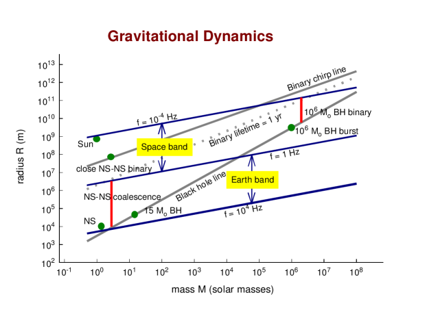
Figure 3: A rough classification of binary systems according to their total mass (horizontal axis) and size (vertical axis). The three solid lines with slope 1/3 in this log-log chart show systems whose natural frequencies $(\pi G\varrho)^{1/2}$ are $10^{-4}$ Hz, 1 Hz, and $10^{4}$ Hz, respectively. These divide the chart into systems in the frequency region that one can observe from space and the ground. The line with slope 1 is the black-hole line: systems below this line do not exist. The dotted line is the line below which systems will coalesce within one year. The solid chirp line, on the other hand, delimits systems that can be observed to change their frequency in one year. Notice that all binaries observable from the ground will coalesce within one year, while most binaries observable by LISA with masses above about 1000 solar masses will chirp.

From these times, it is possible also to calculate the population statistics of chirping systems if they are created at a fixed steady rate $R$ and die away through coalescence. Then the steady-state population of systems radiating gravitational waves with a frequency larger than any given $f_{\text{gw}}$ is

$$N(>f)=7000\left(\frac{f_{\text{gw}}}{0.1\text{mHz}}\right)^{-8/3}\left(\frac{{\mathcal{M}}}{1.2M_{\odot}}\right)^{-5/3}\left(\frac{R}{10^{-5}\text{yr}^{-1}}\right).$$ (11)

For example, in the Galaxy, systems like the Hulse-Taylor pulsar are expected to form once every $40^{5}$ yr or so, so this means that there should be thousands of such systems within the LISA waveband. LISA should certainly see many if not most of them, depending on whether they are obscured by radiation from the far more common white-dwarf binary systems.

Another interesting number is to try to estimate the population of binaries of $1000M_{\odot}$ that might be observable by LISA. LISA should see any chirping system in its waveband anywhere in the Universe. In the first generation of stars, suppose that 10% of the present stellar mass of the universe went into such stars during a time lasting about $10^{9}$ years. Then there would have been some $10^{18}$ such stars that formed. Most of them may well have evolved into black holes [14], and the gravitational collapse event might not have disrupted the binary system. Any such binaries with a local gravitational wave frequency above 6 mHz would, by the above formulas, coalesce within about 1 year of our time, so LISA could follow the event most of the way to coalescence.

Suppose a fraction $\eta$ of such systems formed binaries that could coalesce in the first $10^{9}$ years. Then the rate of formation of such binaries was $10^{9}\eta$ per year. By (11), the number of such systems that LISA could follow to coalescence in one year of observing is about $1700\eta$. So if the efficiency of formation of these binaries is better than one tenth of one percent, then LISA would be able to detect a few. If the efficiency is better than 1%, then LISA would have of order 200 events during a ten-year mission lifetime, and the upper limit on the luminosity distances to these events would signal the onset of this first generation of star formation.

4 Cosmology with Ground-Based Detectors

The use of chirping binaries as standard candles to discover cosmological information has been studied by a number of authors [12, 15, 16, 17, 18]. They have pointed out that there is a variety of methods to avoid the problem of identifying the galaxy in which the chirp occurred, and still extract cosmological information. I begin here, however, with the expectation that chirps may produce gamma-ray bursts, and in any case should certainly produce optical/radio/X-ray displays of some kind, which I will call “afterglows”. These will help the identification of the event. After this discussion, I return to the subject of identifying black hole coalescences, which should have no optical counterpart.

4.1 Afterglow cosmology

As we have noted above, the second-generation ground-based detectors should have ranges so that confident detections of coalescences of binary neutron stars can be made out to 400 Mpc or so. Tens of events per year are to be expected [19]. However, the errors in position determination are rather large, so that if no other information is available then it will be difficult to determine the galaxies in which the event occurred.

The situation will be dramatically different if such events lead to gamma-ray bursts, or indeed if they lead to any other kind of transient event that leaves behind an afterglow. This seems very likely. From the identification of the event by electromagnetic detection of the afterglow, the position can be determined with very small errors and the redshift of the galaxy can be measured. Then the luminosity distance can be determined within errors given just by the SNR, which could be of order 10. Thus, each event leads to a value for the Hubble constant accurate to 10%. With 50 events over a few years of observing, the statistical errors could go down to a few percent. Although the Hubble constant should be known to this accuracy by other means by the time second-generation detectors operate, this method will be an important check on the systematics of other determinations.

Being able to give advance notice of a burst event by gravitational waves will also be a valuable contribution of these detectors. The gravitational wave signal will precede even the gamma-ray burst, and the detector scientists plan to build early-warning alert systems so that notice of potential events could be available to cooperating astronomers within seconds of the gravitational wave observation. In advanced detectors, the inspiral signal for two neutron stars could last several minutes, and there could be enough signal after the first minute to predict the coalescence event. In this case, astronomers would have a minute or so notice to begin observing before the actual coalescence event even occurred.

The association of gravitational wave events with afterglows will of course immensely help modelling of gamma-ray bursts, and it will also allow estimates of the beaming fraction. Gravitational wave emission by these systems is much more isotropic than the gamma radiation, and therefore detectors should give a fair sample of all coalescing systems within their range.

It is possible that gamma bursts are associated more strongly with coalescences between neutron stars and black holes than between double neutron stars. If this is the case, the second-generation detectors will have a longer range, out to redshifts of order 0.3. This will make their ability to do cosmology much more interesting, and measurements of the local acceleration of the universe to $\pm 10$% would be possible over 5 years.

All of these numbers improve by factors of 2 or more if a further detector is added to the network, say in Japan.

4.2 Cosmology with binary black hole observations from the ground

It is possible that the event rate for coalescence of binary black holes of stellar mass will be comparable to that for binary neutron stars. Binaries are less likely to be disrupted by black-hole formation than by neutron-star formation because less mass is lost. And globular clusters seem to be efficient factories for black-hole binaries [20]. It may happen, then, that the first events detected by ground-based instruments will be black-hole coalescences. And if that is the case, then second-generation detectors may see many tens of such events out to redshifts of order 1. Over this distance, it is no longer appropriate to speak of the Hubble constant or the deceleration parameter, since these are just terms in the Taylor expansion of the recession velocity. The observed acceleration of the universe makes such a local approximation inadequate. The goal over cosmological distances is to sample the function $z(d_{L})$, the Hubble flow, over as large a range of values of $d_{L}$ as possible.

Unfortunately, distant as these black-hole events are, they do not produce afterglows or other electromagnetically detectable counterparts from which a redshift can be measured. To circumvent this, I have proposed a statistical method [12] that can still measure the parameters describing the Hubble flow over this interesting distance range. The method is interesting not only because it can determine parameters, but also because it is an example of a nonlinear statistical method whose errors improve much more rapidly with the number $N$ of samples than the usual $N^{1/2}$ associated with linear averaging, at least at first when $N$ is small.

The idea is best illustrated for low-redshift measurements, where the goal is simply to determine one number, the Hubble constant. After understanding how this is done, we will see how it could be generalised to larger redshifts. For each event, the detectors will produce an error box on the sky with a number of candidate clusters of galaxies in which the event may have occurred. The angular position of each candidate leads to a corresponding luminosity distance; measuring the mean redshift of each cluster then leads to a “candidate” value of the Hubble constant for that cluster. Each candidate cluster produces a candidate value. Most are wrong, but one of them should be the correct one. Now, if one has, say, ten such events, then one value of the Hubble parameter should appear in each set of candidates. As long as the number of candidate values is not so large that the observational errors create a lot of overlap between false and true values, it should be possible to zero in on the correct value of the Hubble parameter and retrospectively identify the clusters in which the events occurred. With dozens of events, this method should be very efficient.

This method is actually a one-dimensional version of the Hough transform method that was devised to analyse bubble-chamber photographs in high-energy physics (see [21]). The tracks expected of particles were parametrised, and the number of bubbles on each possible track was counted. Real tracks would have a much larger number of bubbles than random ones. The Hough transform is now being developed to search for unexpected pulsar signals in gravitational wave data [22].

For high-redshift objects, one could use the Hough transform to search for the best set of parameters for a cosmology. Appropriate parameters might be the present Hubble constant, the value of $\Omega_{\text{matter}}$, and the value of $\Lambda$. With many tens of events, there should be enough statistics to find a set of values that all the observations are consistent with. Of course, if by then the Hubble constant is well-enough known to determine the correct candidate from among the candidate clusters of galaxies, then this statistical method is not needed.

Once the clusters containing the events are established, then the redshift and the luminosity distance can be used to calibrate the expansion of the universe. At this point the statistical errors of the measurements of the large number of events will indeed reduce as $1/\sqrt{N}$. With data out to $z=1$, the parametrisation of the Hubble flow will be sensitive to the turnover, where the universe changed from deceleration to acceleration. We shall see that LISA can extend this method to redshifts of 4 or more.

5 Cosmology with LISA

LISA could measure a few mergers of massive black holes in the centres of galaxies each year. It will be sensitive to masses in the range $10^{3}$–$10^{7}\,M_{\odot}$. These observations will give important insight into the processes that formed the black holes, into their population statistics, and into the role they played in galaxy formation. But here I wish to focus on the use of LISA to measure the Hubble flow itself.

For a typical system of two $10^{6}\,M_{\odot}$ black holes at $z=1$, LISA on its own will be able to determine the position to an accuracy of about half a degree. The physical size of the error box will be of the order of 40 Mpc in all three dimensions, because LISA’s distance determination is also limited by the angular errors, as explained earlier. Thus, the error box is about 1% of the distance to the source.

This error box may contain a number of rich clusters, each with one or more candidate galaxies that show evidence of a past galaxy merger that could have led to the black hole merger. We would like to identify the cluster in which the merger took place. There are at least three ways to do this.

1. If by the time LISA flies, the Hubble flow is known to an accuracy of better than 1% out to redshifts of 4 or so, then this may assist identifying the cluster. One measures the redshifts of each of the candidates, and uses the angular positions of the candidates to determine from the LISA chirp signal what the luminosity distance is to that candidate. If the Hubble flow is known accurately as a function of luminosity distance, then the expected redshift can be compared with the measured one, and if these do not coincide then the candidate can be rejected. If the expansion is known well enough, then the candidates may be narrowed down to just 1.

2. If the expansion is not known to this accuracy by the time LISA flies, then the statistical method described in the previous subsection could be brought to bear. This could work if there are of order ten events at high redshift over the mission lifetime of 10 years. The goal at this stage would be to determine the Hubble flow accurately enough to identify the galaxies in which the events have taken place.

3. Failing both of these circumstances, it will be a challenge to observers and astrophysicists to determine the galaxy in which the merger occurred by other means. Perhaps the morphology of the galaxy is special in some way. The gradual in-spiral of the two massive black holes transfers considerable energy to a number of stars in the core of the galaxy, and so it may be that the central bulge of this galaxy has a larger number of stars on nearly radial orbits than is normal. Or perhaps the two black holes maintained accretion disks, or even jets, until they came close enough to one another for tidal forces to disrupt them. The fossil jets may still be visible in the outer regions of the galaxy, and the gas of the accretion disks may have been expelled or shocked in a way that is observable for some time after the disruption.

The identification of the merger galaxies has a large potential payoff. The accurate angular position for each galaxy will provide a very accurate value of the luminosity distance, perhaps with errors smaller than 0.1%, depending only on the SNR of the detection. With the measured redshifts, then the measurements of the Hubble flow are limited only by the proper velocities of the galaxies (inducing single-measurement uncertainties in the Hubble flow of 0.1%). With a handful of merger events spread over redshifts out to, say, 4 or more, it should be possible to go well beyond $\Lambda$-cosmology models and test quintessence and other models in which the pressure is not strictly equal to the negative of the energy density, and in which the density of dark energy/negative pressure is variable in time.

6 Stochastic gravitational waves from the Big Bang

Probably the most fundamental cosmological observation that gravitational wave detectors can make is of gravitational waves coming from the Big Bang. This is the gravitational analogue of the cosmic microwave background radiation, but with a key difference. Because gravitational waves couple so weakly to matter, they never thermalised. The non-thermal spectrum comes to us unchanged from whatever event(s) produced it. Using gravitational waves we can see directly to the first fraction of a second after the Big Bang.

Unfortunately, what firm predictions exist for the amount of radiation that is produced by the Big Bang are discouraging. Gravitational waves should be created at some level by inflation in the same processes that produced the fluctuations in energy density that led to galaxy formation, but the present energy density must be less than $10^{-13}$ of the closure density. The only observational limits are from the millisecond pulsar at frequencies of 1 cycle per 10 years, and from the requirement that the radiation not disturb nucleosynthesis. In both cases the limits require $\Omega_{\text{gw}}$ to be smaller than about $10^{-6}$.

Between the prediction of inflation and the observational limits there is lots of room for other creative mechanisms, and many exist. Toy models of superstring cosmology can produce tailor-made spectra with large amounts of radiation. Cosmic defects, phase transitions, and other unknown but not implausible physics can lead to radiation confined to certain wave-bands. Even brane-world cosmologies have the potential to produce radiation up to the nucleosynthesis limit at any frequency [23].

Ground-based detectors can see this radiation best by cross-correlating the outputs of two nearby detectors. The best suited are the two LIGO instruments. In the second generation they may reach as low as , perhaps a little lower. LISA cannot cross-correlate its two independent interferometers because they share a common arm and hence common noise. It can, however, internally calibrate its instrumental noise and thereby identify any stochastic gravitational wave signal whose power is comparable to or larger than the instrumental noise. This is unlikely to take it lower than $\Omega_{\text{gw}}\sim 10^{-10}$. I have proposed a variant of the LISA mission that could go down as low as $10^{-13}$, but this still does not reach the inflation prediction. A future LISA follow-on mission would be required to reach that level.

One of the problems with detecting a background from the Big Bang is that there are astrophysical backgrounds of a more recent origin. This includes radiation from white-dwarf binary systems, ordinary binaries, close neutron-star binaries, and even small objects falling into massive black holes. There could be a window around 1 Hz where the astrophysical backgrounds are weak enough to allow the cosmological background to dominate, but there are believed to be few other accessible windows [24].

Only observations will tell us what is out there. LISA will certainly measure the compact white-dwarf binary background, which is expected to stand out well above the noise below 1 mHz. LISA might also measure backgrounds at higher frequencies. Whether LISA or the ground-based detectors manages to see a cosmological background from fundamental physics near the Big Bang is one of the most unpredictable outcomes of gravitational wave astronomy.

7 Conclusions

The astronomical community has waited a considerable time for gravitational wave detectors to realise their promise. The progress has been steady but largely invisible until now. From next year, detections of some systems will be possible. But cosmological returns are likely to require another decade of development.

The second-generation ground-based detectors should make the first impact on cosmology, providing values for the Hubble constant and the acceleration of the universe that with an accuracy competitive with that of other methods. This will be a useful check on all methods. The opening up of the low-frequency window by LISA after 2011 will bring much larger potential payoffs for cosmology. With some luck (or cleverness!), LISA could measure the deceleration/acceleration history of the universe with outstanding accuracy out to redshifts of 4 or earlier. To realise this promise, coordinated observations with telescopes in the optical/IR, X-ray, radio, and other bands will be essential.

References

- [1] P. R. Saulson: Fundamentals of Interferometric Gravitational Wave Detectors (World Scientific, Singapore, 1994)
- [2] J Hough, S Rowan: Living Rev. Relativity 3, 3 (2000). [Online article]: http://www.livingreviews.org/Articles/Volume3/2000-3hough/ (cited on 20 November 2001)
- [3] C. W. Misner, K. S. Thorne, J. L. Wheeler: Gravitation (Freeman & Co., San Francisco, 1973)
- [4] B. F. Schutz: A First Course in General Relativity (Cambridge University Press, Cambridge, 1985)
- [5] B. F. Schutz, C.M. Will: ‘Gravitation and General Relativity’. In: Encyclopedia of Applied Physics 7, 303-340 (1993)
- [6] B F Schutz: ‘Gravitational Radiation’. In: Encyclopedia of Astronomy and Astrophysics (Institute of Physics Publishing, Bristol, and Macmillan Publishers Ltd., London, 2000). Electronic version: gr-qc/0003069.
- [7] B. F. Schutz, F. Ricci: ‘Gravitational Waves, Sources and Detectors’, in: Gravitational Waves, ed. by I. Ciufolini, V. Gorini, U. Moschella, P. Fr (Institute of Physics Publishing, Londo, 2001).
- [8] B. F. Schutz (ed): Classical and Quantum Gravity, 18, Number 19 (7 October 2001).
- [9] K. S. Thorne: “Gravitational Radiation”. In: 300 Years of Gravitation, ed. by S. W. Hawking, W. Israel (Cambridge University Press, Cambridge, 1987), pp. 330–458
- [10] C. Cutler, E. E. Flanagan: Phys. Rev. D49, 2658 (1994)
- [11] A. Vecchio, C. Cutler, In: Recent developments in theoretical and experimental general relativity, gravitation, and relativistic field theories, pt. B, ed. by T. Piran (World Scientific, Singapore, 1999), pp. 1121–1123
- [12] B.F. Schutz: Nature 323, 310 (1986)
- [13] L. S. Finn, D. F. Chernoff: Phys. Rev. D 47, 2198 (1993)
- [14] I. Baraffe, A. Heger, S. E. Woosley: Astrophys. J. 550, 890 (2001)
- [15] D. Markovic: Phys. Rev. D 48, 4738 (1993)
- [16] D F Chernoff, L. S. Finn: Astrophys. J. 411, L5 (1993)
- [17] L. S. Finn: Phys. Rev. D 53, 2878 (1996)
- [18] Y. Wang, E. L. Turner: Phys.Rev. D 56, 724 (1997)
- [19] D. R. Lorimer, E. P. J. van den Heuvel: Mon. Not. Roy. astr. Soc. 283, L37 (1996)
- [20] S. F. Portegies Zwart, S. L. W. McMillan: Astrophys. J. 528, L17 (2000)
- [21] V. E. Leavers: CVGIP: Image Understanding, 58, 2, 250 (1993)
- [22] B. F. Schutz and M.-A. Papa In: Proceedings of Jan 1999 Moriond meeting ”Gravitational Waves and Experimental Gravity”, ed. by J. Tr n Thanh V n, J. Dumarchez, S. Reynaud, C.Salomon, S. Thorsett, J.Y. Vinet (Hanoi, 2000). Electronic version: gr-qc/9905018.
- [23] C. J. Hogan: Class. Quant. Grav. 18, 4039 (2001).
- [24] C. Ungarelli, A. Vecchio: Phys. Rev. D 6306 4030 (2001), art. no. 064030